Wave-packet Formalism of Full Counting Statistics

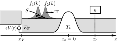
In this paper, we make extensive use of the first-quantized formulation of the generating function: starting with a simple one-particle problem, we exploit the equivalence between the notion of fidelity and full counting statistics. [4] Consider an incoming wave packet $\psi(x;t\to-\infty)$ from the left of the form

with normalization $\int(dk/2\pi)|\phi_{1}(k)|^{2}=1$, cf. Fig. 1. In the following, we assume (for simplicity) a linear spectrum $\epsilon=v_{\scriptscriptstyle\rm F}k$ with $v_{\scriptscriptstyle\rm F}$ the Fermi velocity; at low temperatures and voltages the interesting physics usually takes place near the Fermi points. The momentum $\hbar k$ and the energy $\hbar\epsilon$ are measured with respect to the Fermi momentum $k_{\scriptscriptstyle\rm F}$ and the Fermi energy $E_{\scriptscriptstyle\rm F}$. Here and below, the wave-packets include only momenta with $k>0$ in order not to disturb the Fermi sea which is considered to be the vacuum in our analysis. The scatterer at $x=0$ is characterized by momentum(energy)-dependent transmission (reflection) amplitudes $t_{k}$ ($r_{k}$; particle reflection takes us to the branch $\epsilon=-v_{\scriptscriptstyle\rm F}k$, with $k$ measured relative to $-k_{\scriptscriptstyle\rm F}$). The spin- (or qubit-) counter, placed to the right of the scatterer, contributes a phase-factor $e^{\pm i\lambda/2}$ to the wave function, where the sign depends on the state $|{\uparrow}\rangle$, $|{\downarrow}\rangle$ of the spin-counter. The outgoing ($t\to\infty$) wave-function assumes the form (we place the counter right behind the scatterer at $x=0$)

and consists of reflected ($x<0$) and transmitted ($x>0$) parts; $\Theta(x)$ is the unit step-function. The fidelity $\chi_{1}(\lambda)$ is given by the overlap of wave functions with slightly different perturbations in their evolution, here, with coupling to opposite spin-configurations $|{\uparrow}\rangle$ and $|{\downarrow}\rangle$,

in the asymptotic or long-time limit, the integration over space is trivially done by exploiting the complete separation of the wave function into transmitted and reflected parts. Furthermore, the time dependence disappears as soon as the transmitted wave function has passed the counter. The transmission probabilities $T_{k}=|t_{k}|^{2}$ are the eigenvalues of the transmission operator $\mathcal{T}=\int(dk/2\pi)T_{k}|k\rangle\langle k|$. Given the above specific coupling to a spin, the fidelity is equivalent to the characteristic function

of the full counting statistics as defined in Ref. 24, where a spin-galvanometer has been used as a measuring device. The Fourier-coefficients $P_{m}$ are the probabilities for transmitting $m$ particles. For the simple example of one incoming particle only two outcomes are possible, particle reflection with probability $P_{0}=1-\langle\mathcal{T}\rangle$ and particle transmission with $P_{1}=\langle\mathcal{T}\rangle$, where $\langle\mathcal{T}\rangle=\langle\phi_{1}|\mathcal{T}|\phi_{1}\rangle$ denotes the average transmission probability. Knowing the characteristic function, the cumulants $\langle\langle n^{j}\rangle\rangle$ can be obtained as the coefficients in the Taylor series of $\log\chi(\lambda)$,

The ratio $F=\langle\langle n^{2}\rangle\rangle/\langle n\rangle$ between the second and the first cumulant, called Fano-factor, will be of special interest later.

Next, we extend the above description to $N$ particles with an incoming wave function $\Psi(\mathbf{k})$ defined in momentum space; the vector $\mathbf{k}=(k_{1},\dots,k_{N})$ specifies the $N$ momenta of the particles. We consider independent particles without interaction which scatter independently. After scattering, the outgoing wave function assumes the asymptotic ($t\to\infty$) form

i.e., the evolution is the product of the single-particle evolutions in expression (7). The characteristic function of the full counting statistics $\chi_{N}(\lambda)=\int\!d\mathbf{x}\,\psi_{\text{out}}^{-}(\mathbf{x};t)^{*}\psi_{\text{out}}^{+}(\mathbf{x};t)$ then can be cast into the form

So far, we did not specify the specific type of incoming wave function. If we limit ourselves to Slater determinant states composed of orthonormalized single particle states $\phi_{m}$,

the expression Eq. (12) can be rewritten as a single determinant (see Eq. (69))

involving the single-particle matrix elements $\langle\phi_{m}|\mathcal{O}|\phi_{n}\rangle$ of the operator $\mathcal{O}=1-\mathcal{T}+\mathcal{T}e^{i\lambda}$.

In a physical realization of such a scattering experiment, one usually does not populate orthogonal states as used in the above construction of the Slater determinant. E.g., in the setup of Fig. 1 the electrons typically occupy states $f_{1}$ and $f_{2}$ with a finite overlap, i.e., they are nonorthogonal. Of course, an $N$-particle Slater determinant can be constructed as well out of nonorthogonal states $|f_{m}\rangle$, provided they are linearly independent, i.e., $\det\langle f_{m}|f_{n}\rangle\neq 0$. The properly antisymmetrized and normalized wave function (13) then acquires the form

Inserting this expression into (12) and repeating the calculation that led to (14), we obtain the generating function in the form of a ratio of two determinants,

with the two $N\times N$ matrices

It turns out that the expression (16) for the generating function can be drastically simplified and rewritten in a generalized binomial form. As a first step towards this goal, one has to realize that an $N$-dimensional Hilbert space $H_{N}$, spanned by the single-particle wave-functions $f_{n}(k)$, defines exactly one properly antisymmetrized wave function, or, equivalently, there exists (up to a phase factor) only one associated $N$-particle Slater determinant state. The antisymmetrized $N$-particle state is thus a property of the Hilbert space $H_{N}$ and is independent on the basis chosen.[30]

Consider, as a simple example, a two-particle Slater-determinant state (in second-quantized notation) $|\Psi\rangle=a_{2}^{\dagger}a_{1}^{\dagger}|0\rangle$, with the vacuum-state $|0\rangle$ and Fermionic operators $a_{1,2}$. Defining the new operators $a_{\pm}=(a_{1}\pm a_{2})/\sqrt{2}$, we easily see that the two-particle state

remains unchanged. Consider then a general $N$-particle Slater determinant state of the form Eq. (15). Transforming the basis states $f_{m}(k)$ to new states $g_{m}(k)$ via the complex linear transformation

the antisymmetric combination

remains invariant up to the factor $\det\mathsf{A}$; here, we have used the fact that the determinant of the product of two matrices is the product of the individual determinants. Furthermore, the normalized $N$-particle Slater-determinant states $\Psi^{f}$ and $\Psi^{g}$ obey the relation

with $\text{sgn}(x)=x/|x|$. The only effect of adopting a new basis is the appearance of an overall phase factor $\text{sgn}(\det\mathsf{A})$ which drops out of the characteristic function (12). Therefore, the full counting statistics calculated in the bases $f$ and $g$ give identical results.

The above invariance can be used to simplify the calculation of the full counting statistics. Furthermore, even without specification of the (time-independent) scatterer, one can obtain valuable insights about the structure of possible outcomes in the counting statistics. In particular, it turns out that the most general full counting statistics for a Slater-determinant state is given by a generalized binomial expression of the form (2).

Let us first investigate how the invariance under linear transformations, Eq. (19), manifests itself in the determinant formula Eq. (16). To this end, we note that any single-particle matrix $\mathsf{B}$ of the form (17) transforms under the linear transformation $\mathsf{A}$ of the basis functions according to

Since $\det(\mathsf{A}\mathsf{B})=\det\mathsf{A}\det\mathsf{B}$, we find that the characteristic function $\chi_{N}$ (we define $\mathsf{X}^{f}=\mathsf{S}^{f}-\mathsf{T}^{f}+\mathsf{T}^{f}e^{i\lambda}$) is invariant under the change of basis,

This invariance can be exploited by going over to new orthogonal basis functions $g_{m}(k)$ with an overlap matrix $\mathsf{S}^{g}_{mn}=\delta_{mn}$ and a transmission matrix assuming a diagonal form $\mathsf{T}^{g}_{mn}=\tau_{m}\delta_{mn}$. The possibility of simultaneous diagonalization of the matrices $\mathsf{T}^{g}_{mn}$ and $\mathsf{S}^{g}_{mn}$ is a consequence of the transformation law (22) characteristic of bilinear forms (as opposed to linear transformations $\mathsf{L}$ which transform according to $\mathsf{L}^{g}=\mathsf{A}^{-1}\mathsf{L}^{f}\mathsf{A}$) combined with the positivity of $\mathsf{S}^{f}$. The corresponding eigenbasis $g_{m}$ and eigenvalues $\tau_{m}$ of $\mathsf{T}^{g}_{mn}$ can be found by solving the generalized eigenvalue problem

with the normalization $a_{m}^{\dagger}\mathsf{S}^{f}a_{m}^{\vphantom{\dagger}}=1$. [31] The eigenvectors $a_{m}$ constitute the column vectors of the transformation matrix $\mathsf{A}=(a_{1},\dots,a_{N})$. The eigenvalues are given by the roots of the characteristic polynomial $\det(\mathsf{T}^{f}-\tau\,\mathsf{S}^{f})=0$. The full counting statistics, Eq. (16), written in the new basis $g_{m}(k)$ assumes the generalized binomial form

where the determinant has been evaluated explicitly and the result depends only on the eigenvalues $\tau_{m}$. The generalized eigenvalue problem can be reduced to a normal one by rewriting the problem in a orthogonalized basis $\phi_{m}(k)$, with $\mathsf{S}^{\phi}=\openone_{N}$, which can be obtained by the Gram-Schmidt procedure or by setting $\phi_{m}(k)=\sum_{n}[(\mathsf{S}^{f})^{-1/2}]_{nm}f_{n}(k)$.

From the above, we see that the concrete form of the eigenvalue problem (24) is basis dependent, whereas the eigenvalues and vectors are simply a property of the transmission operator $\mathcal{T}$ operating in the Hilbert space $H_{N}$ with the scalar product $\langle f|g\rangle$. Indeed, it is possible to find the eigenvalues and eigenvectors in a basis independent way using the positive definite quadratic forms $T(g)=\langle g|\mathcal{T}|g\rangle$ and $S(g)=\langle g|g\rangle$, $g\in H_{N}$. Representing the bilinear form $T(g)$ with fixed $S(g)=1$ as a polar plot with $T(g)$ the radius and $g$ defining the direction in $H_{N}$, we obtain an ellipsoid in $N$-dimensional space. The lengths of the main axes of this ellipsoid then constitute the eigenvalues and the associated directions the eigenvectors of the problem (24). [32] The eigenvalues $\tau_{m}$ are constrained to the interval $[0,1]$ as $T(g)\geq 0$ and $T(g)\leq S(g)$ due to unitarity.

The above discussion has concentrated on incoming states described by a single Slater determinant, i.e., nonentangled states with Slater rank 1. It is instructive to generalize this discussion to entangled states involving a coherent superposition of Slater determinants. We start from an incoming state of $N$ particles with Slater rank 2,

where $\Psi^{\text{I}}(\mathbf{k})$ and $\Psi^{\text{II}}(\mathbf{k})$ are normalized $N$-particle Slater determinants describing particles incoming from the left and made from single particle states $f^{\text{I}}_{m}(k)$ and $f^{\text{II}}_{m}(k)$, $m=1,\dots,N$; the complex numbers $\alpha$ and $\beta$ have been chosen such as to make $\Psi(\mathbf{k})$ normalized. The characteristic function for the full counting statistics (12) assumes the form

where Re denotes the real part. The first two terms reduce to generating functions for simple Slater determinant states and we can write

with

The matrices with superscripts $f^{\text{I}}$ and $f^{\text{II}}$ have been defined in Eq. (17), while the new Hermitian matrices with a superscript ‘mix’ are given by the mixed matrix elements

The first two terms in (28) can be diagonalized as before, cf. (24),

with the eigenvalues $\tau^{\text{I}}_{m}$ and $\tau^{\text{II}}_{m}$ given by the roots of $\det(\mathsf{T}^{\text{I}}-\tau^{\text{I}}\mathsf{S}^{\text{I}})=0$ and $\det(\mathsf{T}^{\text{II}}-\tau^{\text{II}}\mathsf{S}^{\text{II}})=0$.

Let us then concentrate on the characteristic function $\chi^{\text{mix}}(\lambda)$. Unfortunately, there is no generic procedure to follow in this case, as the matrices $\mathsf{S}^{\text{mix}}$ and $\mathsf{T}^{\text{mix}}$ are not Hermitian any more and hence the expression (27) cannot be further simplified in general. In particular, the characteristic function $\chi^{\text{mix}}(\lambda)$ is not invariant under individual transformations of the bases $f^{\text{I}}_{m}$ and $f^{\text{II}}_{m}$ (such basis transformations leave the Slater-determinants invariant only up to a phase factor, which dropped out in the calculation of the characteristic function of a single Slater determinant state but does not when two Slater determinants are superimposed coherently). In order to proceed further, we restrict ourselves to specific situations where $\mathsf{S}^{\text{mix}}=0$ or $\det\mathsf{S}^{\text{mix}}\neq 0$. The most trivial case is realized for mutually orthogonal sets of basis functions $f^{\text{I}}_{m}$ and $f^{\text{II}}_{m}$ where $\mathsf{S}^{\text{mix}}=0$; if, in addition, $\det\mathsf{T}^{\text{mix}}=0$, we have $\chi^{\text{mix}}(\lambda)=0$ (see also Sec. III.3 below), else $\chi^{\text{mix}}(\lambda)=\tau^{\text{mix}}(e^{i\lambda}-1)^{N}$ with $\tau^{\text{mix}}=\det\mathsf{T}^{\text{mix}}/\sqrt{\det\mathsf{S}^{f^{\text{I}}}\mathsf{S}^{f^{\text{II}}}}$.

Second, let us assume that $\mathsf{S}^{\text{mix}}$ is invertible, $\det\mathsf{S}^{\text{mix}}\neq 0$. Let $\tau^{\text{mix}}_{m}$ be the roots of the polynomial

The matrix $\mathsf{T}^{\text{mix}}(\mathsf{S}^{\text{mix}})^{-1}$ then can be brought into a Jordan canonical form with $\tau^{\text{mix}}_{m}$ on the diagonal and the characteristic function assumes the simple form

The procedure outlined above is straightforwardly generalized to states with higher Slater rank.

The above findings have interesting generic consequences for the charge transport of fermionic particles; in the following, we discuss the simplest case of two particles, see Fig. 1, where nontrivial exchange properties manifest themselves. For $N=2$ particles the diagonalization (24) can be carried out explicitly for arbitrary matrices $\mathsf{T}^{f}$ and $\mathsf{S}^{f}$. The two eigenvalues $\tau_{1,2}$ are given by

where the parameter $2\alpha\!=\!\mathsf{S}_{22}^{f}\!\mathsf{T}_{11}^{f}\!+\!\mathsf{S}_{11}^{f}\!\mathsf{T}_{22}^{f}\!-\!2\text{Re}(\mathsf{S}_{12}^{f}\!\mathsf{T}_{21}^{f})$. Alternatively, the eigenvalues $0\leq\tau_{m}\leq 1$ are given by a minimum/maximum property [32]

with the eigenvectors $g_{1,2}(k)$ given by those functions where the minimum/maximum values are attained, i.e, $T(g_{1,2})=\tau_{1,2}$. Once the eigenvalues $\tau_{m}$ are known, the characteristic function $\chi_{2}$ assumes the simple generalized binomial form

As a result, we find that in the new basis $g_{m}$, the two particles traverse the scatterer independent of one another, i.e., the characteristic function is a simple product of independent one-particle characteristic functions. Even more, the characteristic function is determined by the Hilbert space spanned by the incoming states $f_{1,2}$ and is independent of the choice of basis. Exchange effects manifest themselves when comparing the result (37) for the Slater determinant $\Psi^{f}\propto\det f_{m}(k_{n})$ with the result $\chi_{2}^{\text{dist}}(\lambda)=(1-\mathsf{T}^{f}_{11}+\mathsf{T}^{f}_{11}e^{i\lambda})(1-\mathsf{T}^{f}_{22}+\mathsf{T}^{f}_{22}e^{i\lambda})$ for distinguishable particles, $\Psi^{\text{dist}}\propto f_{1}(k_{1})f_{2}(k_{2})$: Exchange effects are absent if both matrix elements $\mathsf{S}^{f}_{21}=\langle f_{2}|f_{1}\rangle=0$ and $\mathsf{T}^{f}_{21}=0$, i.e., for orthogonal initial and transmitted states. On the other hand, a finite overlap of at least one pair of these states generates finite exchange effects via the substitution of $\mathsf{T}^{f}_{mm}$ in $\chi_{2}^{\text{dist}}$ by the eigenvalues $\tau_{m}$ in $\chi_{2}$.

The minimum/maximum property described above entails a set of a priori inequalities for the transmission probabilities $P_{n}$ involving the transmission matrix elements $T_{\text{min}}=\min\{\mathsf{T}_{11}^{f},\mathsf{T}_{22}^{f}\}$ and $T_{\text{max}}=\max\{\mathsf{T}_{11}^{f},\mathsf{T}_{22}^{f}\}$; note that while the probabilities $P_{n}$ do account for exchange effects, the single particle matrix elements $\mathsf{T}_{mm}^{f}$ obviously do not. With initial (nonorthogonal) wave packets $f_{m}$ normalized to unity, $S(f_{m})=1$, the search for the extrema in Eq. (36) includes these states as well. We then obtain the set of inequalities $0\leq\tau_{\text{1}}\leq T_{\text{min}}\leq T_{\text{max}}\leq\tau_{\text{2}}\leq 1$. Using them to estimate $P_{0}=(1-\tau_{1})(1-\tau_{2})\leq(1-\tau_{2})$, $P_{2}=\tau_{1}\tau_{2}\leq\tau_{1}$, and $P_{1}=1-P_{0}-P_{2}$, we can derive the following bounds

for the transmission probabilities for two particles. The above bounds set an upper limit on bunching ($P_{2}$ and $P_{0}$) and a lower limit on anti-bunching ($P_{1}$). Note though, that the bound on $P_{2}$ does not exclude an increase (due to exchange) of the transmission probability beyond the ‘classical’ value $P_{2}^{\text{dist}}=\mathsf{T}^{f}_{11}\mathsf{T}^{f}_{22}$ for distinguishable particles, see $\chi_{2}^{\text{dist}}$ above. Indeed, since $\mathsf{T}^{f}_{11}\mathsf{T}^{f}_{22}\leq T_{\text{min}}$, a value $P_{2}\gg\mathsf{T}^{f}_{11}\mathsf{T}^{f}_{22}$ remains possible. Such a result has been recently observed:[33] the probability of two-electron events in the electron emission from a $\text{Cs}_{3}\text{Sb}$ photocathode in a photomultiplier tube has been found to be much larger than the square of the probability for single-electron emission. This was observed both in the case of thermal emission without photocathode illumination and photoemission under weak photocathode illumination. Furthermore, as detailed calculation shows, a large $P_{2}$ can also be obtained for wave packets with amplitudes $f_{2}(k)=f_{1}(k+\delta k)$ shifted in $k$-space and a large overlap integral $\mathsf{S}^{f}_{21}$, combined with a transmission amplitude suppressing $k$-values in the overlap region.

An arbitrary two-particle scattering process is fully characterized by the three parameters $P_{0},P_{1},P_{2}$, from which only two are independent; here, we assume that we can transmit only integer charges (no charge fractionalization). In Figs. 2(a) and (b), we find the regions with different statistical properties that can be generated in a two-fermion scattering process, both in $P_{0}$-$P_{2}$ parameter space as well as in the noise $\langle\langle n^{2}\rangle\rangle$ versus average number $\langle n\rangle$ diagram. We start with the definition of the physically accessible regime in these diagrams: requiring that $P_{1}=1-P_{0}-P_{2}\geq 0$ (Fig. 2(a)) and $P_{0},~P_{1},~P_{2}\geq 0$ (Fig. 2(b)), we find that the black regions are forbidden.

Traditionally, starting from Poissonian statistics ($F=1$) relevant for the coherent light emitted from a laser or for the transport of a classical electron gas in a vacuum tube, much emphasis has been put on the distinction between sub- and super-Poissonian statistics, with reduced and enhanced noise intensity as quantified by Fano factors $F<1$ (sub-Poissonian noise) and $F>1$ (super-Poissonian processes). It appears to us that in the context of degenerate fermions, the generic starting point is the binomial statistics, instead, and more relevant qualifications are given by the regimes of sub-binomial and super-binomial processes introduced below.

Nevertheless, let us start our analysis with the traditional classification comparing a process with Poissonian statistics, which is realized on the dotted line in Fig. 2(a) defined through the relation

i.e.,

Within the dark-gray region noise is super-Poissonian, which is usually associated with the bunching of particles and therefore with bosonic statistics. Note that Fano-factors larger than the Poissonian value 1 require a large reflection probability $P_{0}>1/2$; only when most of the particles are reflected one can observe the ‘bunching’ of the remaining transmitted objects.

A much more natural classification for our fermion system is in terms of (deviations from) binomial statistics. The characteristic function $\chi_{2}$ for two fermions in a Slater determinant state can be cast into the generalized binomial form Eq. (37), which depends on two parameters $\tau_{1},\tau_{2}$. As a consequence, the probabilities satisfy the additional inequality

This condition follows from expressing the parameters $\tau_{1},\tau_{2}$ through the probabilities $P_{0},P_{2}$ using the relations $P_{0}=(1-\tau_{1})(1-\tau_{2})$ and $P_{2}=\tau_{1}\tau_{2}$; requiring a positive discriminant of the resulting (quadratic) equation implies the constraint (41) which defines the light gray region in Fig. 2(a)), naturally termed the ‘sub-binomial’ regime. The (thick) black line bounding the general binomial (or sub-binomial) region is the line of usual binomial statistics, which is realized for the case of degenerate transmission coefficients $\tau_{1}=\tau_{2}$ as they appear if the scattering does not depend on energy.

The region with super-Poissonian noise (dark gray) and the sub-binomial region (light gray) are distinct, with the statistics of fermions incoming in a Slater-determinant state always residing in the sub-binomial domain. Note that the counting statistics of an arbitrary two-particle process (without specification of exchange properties) also depends on two out of the three parameters $P_{0},P_{1},P_{2}$ (as the constraint $P_{0}+P_{1}+P_{2}=1$ needs to be fulfilled) but cannot be cast into the form Eq. (37) in general, hence these processes are devoid of such an additional restriction.

The $P_{2}$-$P_{0}$ diagram can be transcribed to the (experimentally more relevant) $\langle\langle n^{2}\rangle\rangle$-$\langle n\rangle$ diagram, cf. Fig. 2(b). The physical constraints $0\leq P_{0},P_{1},P_{2}$ lead to the set of inequalities,

which can be cast into the more compact form $(m+1-\langle n\rangle)(\langle n\rangle-m)\leq\langle\langle n^{2}\rangle\rangle\leq\langle n\rangle(2-\langle n\rangle)$, with $m=0,1$. The single large- and two small parabolas bounding the unphysical (black) regions are given by the second and the two (for $m=0,1$) first inequalities. For the generalized (or sub-) binomial statistics, the additional constraint assumes the form

with the equality applying to the binomial case with $\tau_{1}=\tau_{2}$. Within the gray region of the diagram the noise is sub-binomial $F\leq 1-\langle n\rangle/2$ and hence trivially sub-Poissonian, $F\leq 1$. Note that noiseless transmission of charge requires that an integer average charge is transmitted.

The generalization of the above analysis to $N$ incoming particles in a Slater determinant state is straightforward. The generalized binomial characteristic function is given by Eq. (2). The positivity of the probabilities $P_{m}\geq 0$, $m=0,\dots,N$ imposes the $N+1$ restrictions on the first two momenta $\langle n\rangle$ and $\langle\langle n^{2}\rangle\rangle$, $(m+1-\langle n\rangle)(\langle n\rangle-m)\leq\langle\langle n^{2}\rangle\rangle\leq\langle n\rangle(N-\langle n\rangle)$, with $m=0,\dots,N-1$, defining a simple generalization of Fig. 2(b) with one large and $N$ small parabolas. In the generalized binomial case, the additional constraint

tells that the incoming Slater determinant states produce a sub-binomial noise statistics. A similar result was found recently[34] in the context of adiabatic pumping. The authors considered a time-dependent scattering matrix in the instant scattering approximation (i.e., an energy independent scatterer) and obtained a generating function in a product form describing a generalized binomial statistics with parameters $u_{m}\leq 0$; the $u_{m}$ relate to our $\tau_{m}$ via $\tau_{m}=(1-u_{m})^{-1}$.

The above discussion for two particles lets us conclude that incoming Slater determinant states generate Fano factors $F\leq 1-\langle n\rangle/2\leq 1$; such states are nonentangled. On the other hand, an entangled two-particle state can be generated with a sum of two Slater determinants; such an entangled state (with $0<\alpha<1$, i.e., a state with Slater rank 2, see Sec. II.6)

is sufficient to generate all possible types of two-particle statistics: we choose the Slater-determinant wave functions $\Psi^{\text{I}}$ and $\Psi^{\text{II}}$ (incoming from the left) such that they occupy different parts of momentum space, e.g., $\Psi^{\text{I}}$ has only components below $k_{\text{c}}$ and $\Psi^{\text{II}}$ above. Furthermore, let the transmission be $T_{1}=T_{k<k_{\text{c}}}$ below $k_{\text{c}}$ and $T_{2}=T_{k>k_{\text{c}}}$ above. For such a setup, all the overlap integrals vanish, e.g., $\int(dk_{1}dk_{2}/4\pi^{2})\Psi^{\text{II}*}(k_{1},k_{2})\Psi^{\text{I}}(k_{1},k_{2})=0$, and we obtain (cf. Eq. (28))

that is, the generating function is simply the weighted sum of the two individual generating functions for the Slater-determinant states. The statistics of such entangled wave functions is described by points in the $P_{2}$-$P_{0}$ diagram of Fig. 2(a) which lie on a straight line between the point $p^{\text{I}}$ for $\Psi^{\text{I}}$ and the point $p^{\text{II}}$ for $\Psi^{\text{II}}$ with $\alpha$ parameterizing the line. Both $p^{\text{I}}$ and $p^{\text{II}}$ are situated on the binomial line, while the line connecting them may enter the super-binomial or even the super-Poissonian region: for example setting $T_{1}=0$ and $T_{2}=1$, the characteristic function is given by $\chi_{2}=\alpha+(1-\alpha)e^{2i\lambda}$ and $F=2\alpha$, which assumes values between zero and two (note that in the limit $\alpha\to 1$, the wave function (45) is of Slater rank 1, but nevertheless, the Fano factor approaches $F=2$. As the Fano factor for $P_{0}=1$ assumes the form 0/0 its value depends on the direction from which $P_{0}=1$ is approached). As simple Slater determinants produce only Fano factors up to $1-\langle n\rangle/2$, a larger value serves as a test for the entanglement of the two particles.[35, 36]. For $N$ incoming particles in an entangled state of rank 2, the analogous construction (cf. II.6) produces a Fano factor $F=N\alpha$ with $0<\alpha<1$, i.e., super-Poissonian statistics can be admitted for sufficiently large $\alpha$.

Next, we consider the situation in the setup of Fig. 1 with incoming particles in normalized states $f_{1}(k)$ and $f_{2}(k)$ with overlap $S=\mathsf{S}^{f}_{21}=\langle f_{2}|f_{1}\rangle$ and carrying a spin $1/2$ degree of freedom. We consider the case of spin-independent scattering, hence the coefficients in $\mathsf{T}^{f}$ depend exclusively on $f_{1}(k)$ and $f_{2}(k)$. The four properly symmetrized states available to the two incoming particles are denoted by $\Psi_{s,m_{s}}(\mathsf{k})$, with $s=0$ the singlet ($m_{s}=0$) state and $s=1$ the three ($m_{s}=-1,0,+1$) triplet states. The degrees of freedom $\mathbf{k}$ involve the momenta $k_{m}$ and spins $s_{m}$ of the particles, $\mathbf{k}=(k_{1},s_{1};k_{2},s_{2})$. The triplet states with $m_{s}=\pm 1$ are simple Slater determinant states

References

- [1] L.S. Levitov and G.B. Lesovik, JETP Lett. 58, 230 (1993).
- [2] L.S. Levitov, H.W. Lee, and G.B. Lesovik, J. Math. Phys. 37, 4845 (1996).
- [3] Yu.V. Nazarov, ed., Quantum Noise in Mesoscopic Physics (Kluwer Academic Publishers, 2003).
- [4] G.B. Lesovik, F. Hassler, and G. Blatter, Phys. Rev. Lett. 96, 106801 (2006).
- [5] A. Peres, Phys. Rev. A 30, 1610 (1984).
- [6] Th. Martin and R. Landauer, Phys. Rev. B 45, 1742 (1992).
- [7] H. Lee and L.S. Levitov, cond-mat/9507011 (1995).
- [8] D.A. Ivanov, H. Lee, and L.S. Levitov, Phys. Rev. B 56, 6839 (1997).
- [9] A.V. Lebedev, G.B. Lesovik, and G. Blatter, Phys. Rev. B 72, 245314 (2005).
- [10] J. Keeling, I. Klich, and L.S. Levitov, Phys. Rev. Lett. 97, 116403 (2006).
- [11] G. Fève, A. Mahé, J.-M. Berroir, T. Kontos, B. Plaçais, D.C. Glattli, A. Cavanna, B. Etienne, and Y. Jin, Science 316, 1169 (2007).
- [12] F. Hassler, G.B. Lesovik, and G. Blatter, Phys. Rev. Lett. 99, 076804 (2007).
- [13] We use the term ‘entangled-state’ for indistinguishable particles in the sense of J. Schliemann, J.I. Cirac, M. Kuś, M. Lewenstein, and D. Loss, Physical Review A 64, 022303 (2001).
- [14] F. Taddei and R. Fazio, Phys. Rev. B 65, 075317 (2002).
- [15] K.E. Cahill and R.J. Glauber, Phys. Rev. A 59, 1538 (1999). Cahill et al. denote their generating function (generating counting probabilities upon taking derivatives) by where their is equivalent to in our article.
- [16] R.J. Glauber, in Quantum Optics and Electronics, edited by C. DeWitt, A. Blandin, and C. Cohen-Tannoudji (Gordon and Breach, New York, 1965).
- [17] S. Braungardt, A. Sen(De), U. Sen, R.J. Glauber, and M. Lewenstein, arXiv:0802.4276 (2008).
- [18] G. Burkard, D. Loss, and E.V. Sukhorukov, Phys. Rev. B 61, R16303 (2000).
- [19] K. Schönhammer, Phys. Rev. B 75, 205329 (2007).
- [20] G. Szegő, Math. Ann. 76, 490 (1915).
- [21] G. Szegő, Comm. Sém. Math. Univ. Lund pp. 228–238 (1952).
- [22] L.S. Levitov and G.B. Lesovik, JETP Lett. 55, 555 (1992).
- [23] G.B. Lesovik and N.M. Chtchelkatchev, JETP Lett. 77, 393 (2003).
- [24] L.S. Levitov and G.B. Lesovik, cond-mat/9401004 (1994).
- [25] I. Neder and F. Marquardt, New J. Phys. 9, 112 (2007).
- [26] D.V. Averin and E.V. Sukhorukov, Phys. Rev. Lett. 95, 126803 (2005).
- [27] B.A. Muzykantskii and Y. Adamov, Phys. Rev. B 68, 155304 (2003).
- [28] A. Shelankov and J. Rammer, Europhys. Lett. 63, 485 (2003).
- [29] J.E. Avron, S. Bachmann, G.M. Graf, and I. Klich, Commun. Math. Phys. 280, 807 (2008).
- [30] C.C.J. Roothaan, Rev. Mod. Phys. 23, 69 (1951).
- [31] In condensed matter theory this statement is made use of in the Bogoliubov-Valatin transformation where the quadratic Hamiltonian is diagonalized while keeping the commutation relations invariant.
- [32] R. Courant and D. Hilbert, Methoden der mathematischen Physik, 4th edition (Springer-Verlag, Berlin, Heidelberg, New York, 1993).
- [33] M.V. Lebedev, A.A. Shchekin, and O.V. Misochko, Quantum Electron. 38, 710 (2008).
- [34] A.G. Abanov and D.A. Ivanov, Phys. Rev. Lett. 100, 086602 (2008).
- [35] M.J.M. de Jong and C.W.J. Beenakker, Phys. Rev. B 49, 16070 (1994).
- [36] F. Bodoky, W. Belzig, and C. Bruder, Phys. Rev. B 77, 035302 (2008).
- [37] We assume that the Hamilton operators and for different times commute. Otherwise a time-ordering operator has to be introduced.
- [38] I. Klich, in Ref. 3.
- [39] B.A. Muzykantskii and D.E. Khmelnitskii, Phys. Rev. B 50, 3982 (1994).
- [40] Yu.V. Nazarov and D.A. Bagrets, Phys. Rev. Lett. 88, 196801 (2002).
- [41] S. Pilgram and M. Büttiker, Phys. Rev. B 67, 235308 (2003).
- [42] R.J. Brown, M.J. Kelly, M. Pepper, H. Ahmed, D.G. Hasko, D.C. Peacock, J.E.F. Frost, D.A. Ritchie, and G.A.C. Jone, J. Phys.: Condens. Matter 1, 6285 (1989).
- [43] E.L. Basor, Indiana Univ. Math. J. 28, 975 (1979).
- [44] W. Schottky, Ann. Phys. (Leipzig) 57, 541 (1918).
- [45] B. Simon, in Geometry, Spectral Theory, Groups, and Dynamics, vol. 387 of Contemporary Mathematics, pp. 253–275 (American Mathematical Society, Providence, 2005).