What are the interactions in quantum glasses?
Abstract
The form of the low-temperature interactions between defects in neutral glasses is reconsidered. We analyse the case where the defects can be modelled either as simple 2-level tunneling systems, or tunneling rotational impurities. The coupling to strain fields is determined up to 2nd order in the displacement field. It is shown that the linear coupling generates not only the usual Ising-like interaction between the rotational tunneling defect modes, which cause them to freeze around a temperature , but also a random field term. At lower temperatures the inversion symmetric tunneling modes are still active - however the coupling of these to the frozen rotational modes, now via the 2nd-order coupling to phonons, generates another random field term acting on the inversion symmetric modes (as well as shorter-range interactions between them). Detailed expressions for all these couplings are given.
I Introduction
One of the most subtle and peculiar problems in condensed matter physics concerns the nature of the ”glass” state, and of the associated glass transition. This problem (described by P. W. Anderson[1] in 1995 as ”the deepest and most interesting problem in solid-state theory”) concerns the overwhelmingly dominant component of the physical world as we experience it, ie., non-conducting solids that are not ordered in regular crystalline arrays. In fact the glass problem actually involves two separate features. One is the remarkable universality displayed in the low- quantum properties[2, 3], and the other is the high- behaviour shown in the vicinity of the glass transition itself[4].
At first glance it seems implausible that these two features of glasses could be related - they occur at very different energy scales. Elsewhere we argue that there may be an interesting connection, which depends on certain novel features of the interactions in these systems. The purpose of the present paper is to investigate the form of these interactions in some detail. We derive a number of new interaction terms, which are presented in the form of two new effective Hamiltonians for neutral glasses, one valid for higher temperatures, the other in the low- limit.
We begin with a brief introductory review of the physics of neutral glasses, particularly in the low quantum regime. We then derive the form of the defect-phonon interaction terms (section II), including both a direct linear coupling to the lattice displacement field, and a coupling to the gradient of this field. We then calculate, in sections III and IV, the effective coupling between defects induced by these interactions. It is shown in section III that the linear coupling not only gives the well-known Ising coupling between the rotational tunneling modes, but also a random field acting on these modes. However there is no such linear coupling between phonons and the ’inversion symmetric defects’ (ones which are symmetric with respect to inversion about the local lattice site). In section IV we calculate the coupling of these defects to gradients of the phonon field, and show that this coupling produces another weaker coupling to a random field generated by the now frozen rotational modes, as well as a short-range coupling between the inversion symmetric tunneling defects.
The main point of the present paper is to find the correct quantitative form of the effective Hamiltonian for these systems, after integrating out the phonons. We end up with an effective Hamiltonian at high which involves only the rotational defects, and then another quite different low- Hamiltonian which describes a set of tunneling inversion symmetric defects, coupled to each other and to the random field generated by the frozen rotational modes; this includes a number of new terms. It turns out that these results have very interesting implications for the physics of glasses, which are discussed in detail in Ref.[5].
I.1 Universalities in the low-T quantum state
The first glass conundrum, strongly emphasized by Leggett[2], is the apparent universality in the low-T properties of a huge variety of disordered systems below a temperature K, regardless of the amount of disorder. The most striking universalities are seen in
(i) the Q-factor for torsional oscillations of the system, which is related to the phonon mean free path and the phonon thermal wavelength by . One finds[3] that shows a pronounced plateau for (down to a lower temperature which decreases with ), and that the value varies over only a factor between many different materials, even though the intrinsic disorder (measured by e.g., defect concentration x) may vary over several orders of magnitude.
(ii) The ”Berret-Meissner ratio” between longitudinal and transverse sound velocities in the same low-T regime. A remarkable linear relationship is found[6] between and , for a variety of materials including amorphous oxide, semiconducting, polymer, metallic, and electrolyte glasses, in which varies by a factor of .
These are only the most striking of the low T universalities - there are others[3, 6]. In recent years the experimental groups of Osheroff[7, 8], Hunklinger[9], and Enss[10] have pushed experiments to very low temperatures [ mK)], and found a host of interesting new results, including intrinsic dipolar ”hole-digging” in the many-body density of states[7], and a remarkable spin coherence phenomenon[9, 10] which comes from nuclear quadrupolar interactions in neutral glasses. The dynamical hole-digging persists to the lowest temperatures, giving ever sharper features in the density of states; it is associated with non-exponential relaxation and ’aging’ behaviour of the dielectric constant of the system. It would be of interest to continue these measurements well into the regime, if possible.
Although we are clearly dealing here with a resonant tunneling phenomenon[11], qualitatively similar to that in tunneling spin systems[12, 13] the glass problem apparently involves cooperative tunneling of at least coupled pairs of tunneling systems[8, 11], and the resulting low-T ”universal” state apparently involves some fundamental new physics. Although a number of theoretical scenarios have been proposed to describe this universal physics[3, 11, 14, 15], most of which argue that it must involve strong coupling between the relevant low- modes, there is no complete consensus at the present time. We note in passing that although the universalities occur in the same temperature range as the well-known regularities[16] in thermal and transport properties in glasses (such as the specific heat , or the thermal conductivity ), these latter can all be understood in terms of the well-known picture[17] of non-interacting two-level systems(TLSs). On the other hand the dynamics of dipolar hole-digging certainly requires interactions for its explanation, between whatever modes are exhibiting low- quantum fluctuations, whether these be pairs of TLSs[11] or some more complicated set of modes[2, 14].
I.2 The high-T glass transition
In most glasses there is actually a glass transition at a temperature much higher than the crossover temperature to the universal quantum regime (typically ). There are several universal features of this transition as well[4], amongst which one may single out (i) the characteristic range of relaxation times in the system, and their characteristic T dependence, summarized in the Vogel-Fulcher scaling law, which shows that the value of we use depends on the timescale in interest; (ii) the ”entropy crisis”, in the range , were is the Kauzman temperature, and where one finds a supercooled glass entropy lower than that of the crystalline solid; and (iii) the existence of highly non-exponential relaxation, and characteristic memory and aging effects, in the vicinity of the glass transition (as noted above, these effects are also found in the low-T quantum regime, both in neutral glasses where universality is seen[8] and in electronic glasses[18]).
At first glance there seems to be no obvious relation between this high-T behaviour, which is characterised by thermally-activated processes of great complexity, and the low-T behaviour. A number of attempts have been made in the last couple of years to give a general theory of the glass transition[14, 19, 20]. Two of them[19, 20] made no connection to the low-T regime, instead concentrating on the vast number of thermally-activated processes coming into play near . The Moore-Yeo theory also makes a very interesting connection between the critical behaviour of supercooled liquids near and Ising spin glasses in a magnetic field.
However, there are several arguments that indicate that there may be a connection between the physics below and that near . The first two are experimental. It was already noticed by Berret and Meissner[6] that the low-T phonon relaxation time shows systematic connection to the values of across the whole range of glasses, with . We have already remarked on the rough proportionality ; and indeed one can argue that the coupling between phonons and the low-T tunneling entities (whatever they may be) is intrinsically related to both and the phonon velocities[14].
These observations suggest that there may be some kind of unified theoretical framework which could describe both the high and low-T properties of glasses. Such a theory would not only be of major interest (answering the question posed by Anderson[1]) but it would also clearly give us a new blueprint for theories of other complex systems. Such a framework has actually been proposed very recently by Lubchenko and Wolynes[14]. In this theory the basic objects are ”tunneling centers” which comprise atomic units, and which can be used to describe both the low-T dynamics and the dynamics near . We note that these ”tunneling entities” are very different from the TLSs that have been used to describe many of the low-T experiments[8, 9, 10, 11, 16], although it is argued that their behavior will be quite similar[14].
I.3 Nature of interactions in glasses
We now come to the question to be addressed by this paper. One might think, in view of the generality of the phenomena discussed above, that they ought to be independent of the detailed nature of the interactions between tunneling entities in the low-T regime. Actually it is widely assumed in the glass literature that it is enough to include only dipolar strain-mediated interaction, with the addition of electric dipolar interactions where necessary. This assumption rests on a number of microscopic calculations done over the years, both for interacting TLSs[11, 21, 22, 23, 24], and for the more complicated systems of discrete rotators that exists in orientational glasses[25, 26, 27, 28]. These calculations (particularly those for orientational glasses) are very lengthy, and for this reason have not been attempted with any generality except by a few authors. Nevertheless, the conclusion has been that the effective interaction between tunneling entities a distance apart is
| (1) |
where is a coupling eV), with both dipolar strain and electric dipole contributions. The length is a typical lattice distance; and we have suppressed an angular factor which has roughly dipolar symmetry. We note that all of the principal scenarios for the low-T behaviour of glasses assume (1) to be true; moreover they rely upon it in an essential way.
But is (1) really correct? In this paper we shall argue that in fact (1) is incomplete, and that the correct form contains extra terms of some importance. These include another term falling off like , which however leads to a random field acting on each tunneling rotator. There are also terms which are weaker and which fall off faster, which would be less important except that they act on 2-level systems that do not see the first random field. The net result of this is that we derive two effective Hamiltonians for the system, one which is valid at higher temperatures around and the other at much lower , apparently around the temperature which defines the crossover to the universal properties.
II Defect-Phonon Interactions
In what follows we will be dealing with neutral glasses, i.e., we ignore metallic and superconducting glasses. This of course still includes the overwhelming majority of materials on earth, from rocks and minerals to a galaxy of insulating compounds (based mostly on transition metals), along with a huge variety of natural and artificial organic systems (including polymers).
In spite of this variety, and regardless of whether one is dealing with a strongly disordered amorphous systems or very weakly disordered systems like substitutional electrolyte glasses, the two interactions of main interest are those involving strain fields and phonons, and those involving the interaction of electric fields with local charge distributions.
II.1 Simple model for Defects
Our tactic in this paper will be to start with a toy model which describes a class of very simple systems, and then argue that the important features of this model can be generalised to a much wider variety of glassy systems.
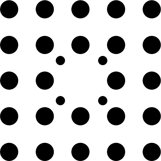

Consider the situation depicted in Fig. 1, in which we reduce the system to a 2-d plane, and look at defects in this plane. The underlying local symmetry of the system is assumed to be of square plaquettes, and the defects can either be substitutional defects, able to occupy one of 4 states in the plaquette, or orientational defects, able to rotate between 4 orientational states. Under certain circumstances, to be discussed below, we can make the ’dumbbell approximation, in which defects rotated by are considered to be indistinguishable - we then treat these 2 states as identical, and the 4-state system reduces to a 2-state system.
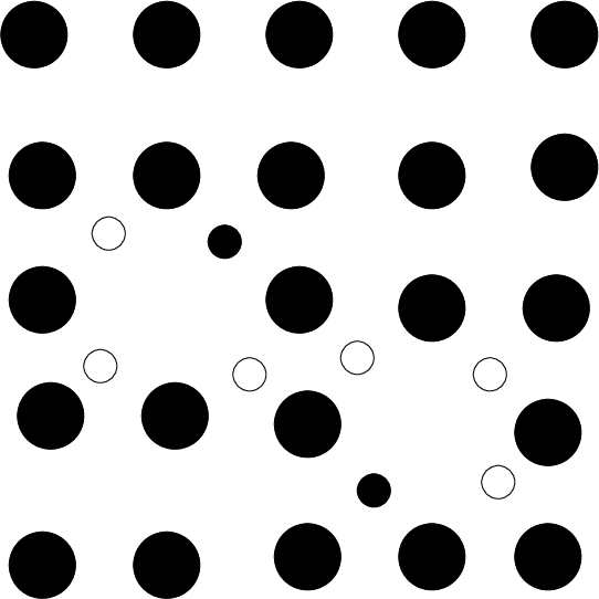
Now if the concentration of these defects is low we can assume that they do not disturb the underlying lattice symmetry, and interactions between 2 defects, even if they are distantly separated, will be between 2 plaquettes which are oriented along the same axes. More generally, when the defect concentration is much higher, one may have the situation shown in Fig. 2, where the 2 plaquettes are slightly distorted, and also rotated with respect to each other.
It might be objected that the situation depicted in Fig. 2 is not very realistic, in that a high defect concentration would so severely disrupt the square symmetry that the plaquettes themselves would not only be rotated, but that their shapes would be severely distorted, so that no clear local lattice structure could be defined. Actually this is not the case - quite surprisingly, the situation in even rather strongly amorphous glasses does not conform to the common caricature in which they look like frozen liquids. Instead, at short length scales the underlying lattice structure is still quite recognizable, and the system more resembles a ’frozen liquid’ of very small polycrystals[29] (actually the instantaneous state of quite a few liquids also looks like this!).
A good tutorial example of systems like our toy model is provided by substitutional electrolyte glasses, where the defects can be characterized very precisely. Canonical examples are , , , and so on[27, 30]. Many experiments in these systems have been done in the very dilute regime, with concentrations in the range x , where one can ignore the interactions between the widely spaced impurities[31, 32, 33]. However there are also many studies of concentrations up to x or even higher. When , interactions between the impurities clearly dominate the physics in most of these systems[30, 33, 34, 35]. This is shown in, e.g., the saturation in the dielectric response for higher concentrations[33].
In real 3-dimensional systems like , , or , one has either off center point-like impurity states (as in , with 8 available positions for the impurity inside a given lattice ’cage’); or else orientational (as in , where the impurity can lie in one of the 8 directions along (1,1,1) and its equivalents). Previous treatments of the microscopic interactions in these systems have taken one of two routes. Michel and collaborators[25, 27] have used a detailed microscopic description of the orientational and translational degrees of freedom (and the coupling between the two of these) with the goal of describing systems where orientational impurities like can rotate inside their host ’cages’. Sethna and collaborators[28, 36, 37] have used a somewhat more general phenomenological description in terms of TLS impurities.
The great advantage of beginning with these simple systems is that one can set up a well-controlled theory beginning with the case of dilute defect concentration . There are good arguments, based on the experiments on electrolyte glasses[30, 31, 32, 33, 34, 35] and other amorphous systems[3, 7, 8, 9, 10, 11, 16], that the theory must, when is larger, flow towards the strong coupling regime (and perhaps to some universal quantum regime). But it makes no sense trying to explore the strong-coupling limit until the form of the interactions has been established in weak coupling. The key question of interest here (viz., what are these interactions?) can only rigorously be addressed by starting from a system where x. Later we will argue that our main results will survive well into the universal regime, and so are of much more general applicability.
Returning now to Fig. 1, we divide the defects into two groups, viz. (i) those in which there is an inversion symmetry relating pairs of states, where inversion is made with respect to the relevant lattice position; and (ii) those where there is no such symmetry. In the square plaquette system we see that both simple impurities like and orientational impurities like or can be in one 4 different states, related by rotations of the plaquette, and there is no inversion symmetry. However in some cases, one can treat the states related by as physically equivalent (either because they really are equivalent, or because at the energy scale of interest the difference is unimportant), and then we can assume inversion symmetry. In this case the state space on the plaquette is 2-dimensional, with states oriented along one or other of the lattice diagonals.
To describe the system, the simplest representation is just a 4-state one in which the system can hop between any of the 4 plaquette sites. However we will use a slightly different one, where we begin by defining a set of operators such that flips the state on the plaquette through , and another set of operators such that rotates the state on the plaquette through in either direction. This representation is used because we will see that the impurity-lattice interaction turns out to depend crucially on whether inversion symmetry is obeyed, and so this way of setting up the description allows us to distinguish between operations which are or are not invariant under inversion symmetry.
In what follows we will first be considering the effect of phonons on the rotational tunneling degrees of freedom. In general, before we take interactions with phonons into account, these will be described by a Hamiltonian
| (2) |
where is a tunneling matrix element and is any stray field acting on the rotational defect variable . At lower , once the rotational degrees of freedom are frozen out, only the inversion tunneling processes are left, and these are described by a bare Hamiltonian
| (3) |
where again an ”external” effective longitudinal field acting on the -th dipole is allowed.
Often, in the study of the possible phases of the system, the high- tunneling is dropped since it is typically too small to influence the nature of the phase, nor its stability to effective random fields[38]. We will keep it simply because we wish to trace how the effective Hamiltonian evolves as we lower the energy scale.
II.2 Coupled Defect-Phonon System
Consider now the coupling to the phonon modes in the system. The Hamiltonian for this system is given by:
| (4) |
where is the bare defect term just discussed, and the phonon system is described by
| (5) |
Here and represent momentum and displacement operators for phonon modes of wave vector and branch , and is the mass of the elementary cell of the medium.
We split the defect-phonon interaction into two terms, writing
| (6) |
where the lowest order term is linear in the phonon displacement field:
| (7) |
and the next term is a non-linear coupling of the defects to the gradient of this field, of form
| (8) |
The linear coupling term contains first a ’volume coupling’ with coefficient , which is independent of the defect position or orientation, arising because the defect has a different volume from the host and this locally strains it. Then there is the usual interaction between the defect and the strain field in the ”TLS” or ”dumbbell” approximation, which changes sign with , since the phonon displacement fields are sensitive to the defect orientation. The size of these interactions is not easy to calculate - however can be measured, and is on a typical scale eV. Estimates of give similar numbers but the ratio must certainly vary from one system to another (calculations are difficult because the volume change and charge redistributions caused by the defect will interact with each other).
We notice that when inversion symmetry is preserved, there is no linear interaction between the and the phonon field. The 2nd term arises when we relax the assumption of inversion symmetry, so states rotated by are distinguishable (either because we relax the ”dumbbell” approximation, and consider the dipole moment of the impurity or molecule, or because we consider tunneling point impurities). In this case the effective ’dipole’ represented by the difference between these states can interact with the gradient of the phonon displacement field, in the form given in . However this interaction is much weaker, and has rarely been considered before. Certainly we do not expect it to affect the physics near the glass freezing temperature. However we will see that this interaction is important at lower temperatures, where other degrees of freedom freeze out. At the present time we cannot give more than a rough estimate for the size of the coefficient of this interaction; noting that its dimensions are (ie., energy times length), and that the characteristic energy scale of defect interaction energies is eV, and the characteristic length scale of defect dynamics is roughly , we would expect that . To get an energy from this we need to divide by the typical distances between impurities, given by , where is a lattice length. Thus we expect that the energy scale associated with this coupling is less than and by a factor . From now on we will assume that this energy scale associated with is considerably smaller than .
III Inter-defect Effective Hamiltonian: High Energies
Let us begin by assuming that we are at a sufficiently high energy scale that we can neglect the weaker interaction ; we are then concerned with a set of phonons interacting with the TLS variables, ignoring the variables. We wish, in this approximation, to calculate the effective Hamiltonian of the system, initially just up to 2nd-order in the defect-phonon coupling. This is an old problem, but we shall see that even here there are new things to be discovered. Let’s look first at the simple problem of 2 interacting defects in this dumbbell approximation. We split the interaction term into two, to understand the effect of the orientation and volume parts separately, and consider 2 defects at positions and . Then the system has bare Hamiltonian:
| (9) | |||||
If we now integrate out the phonons we will generate, at lowest order in , terms of Ising form (proportional to ), cross terms giving a local field, proportional to , plus an energy shift . The Ising form has been known for a long time. The second term, when summed over all spins apart from one given spin, simply leads to a random field at the site of that spin - this term is not usually considered. In this section we first sketch the derivation of the Ising term, primarily to establish notation, and then derive the random field term.
III.1 Ising interaction term
We define the Fourier transformation to momentum space as
| (10) |
where is a phonon polarisation index. Then we have
| (11) |
To find the interaction in 2nd-order perturbation theory we minimize the potential energy, i.e. the sum of the second term in Eq.(5) plus the interaction term. Straightforward calculation results in energy terms proportional to and the Ising interaction term of interest, proportional to . Let us define the notation , and use an acoustic approximation, in which the longitudinal phonon frequency , the transverse phonon frequency is . We also have the identities:
| (12) |
Then the Ising interaction , where
| (13) | |||||
Summing over polarization indices gives
| (14) | |||||
which when the sum over momenta is performed, gives the real space form
| (15) |
with the interaction
| (16) | |||||
Here the reduced variable , and we suppress the ”” subscript on and to keep things uncluttered. This interaction has a rather complicated angular dependence, coming both from the anisotropy of the medium, and from the that of the strain interaction . If we assume a completely isotropic medium with degenerate longitudinal and transverse phonons, and also make the simplification of anisotropic , so that , we get the strictly dipolar form
| (17) |
where is the angle between the unit radius vector and the -axis; the characteristic coupling energy is now evident.
As noted before, these results are well-known, and were first derived[21, 22] in the 1970’s. The essential result is that one has derived an effective Ising interaction; since the sites of the defects are random, the tunneling terms make this system behave as a quantum Ising model with random interactions, and Hamiltonian
| (18) |
where the tunneling amplitudes are typically much smaller than the nearest-neighbour Ising interactions. However it turns out that this Ising interaction is not the only term that is important.
III.2 Random Field term
We now include the cross-terms , coming from 2nd-order perturbation theory in the interaction in Eq.(9). Using similar manouevres as in the calculation above, one now obtains another term in the effective interaction of form , where
| (19) |
We call this a random field term because if we take a given spin in the system, say , and then sum the interaction between and the volume terms coming from all the other defect sites , we get a field acting on at site which varies from site to site in a random way, because of the random positions and orientations of the arguments . Note, incidentally, that this effective random field interaction has contribution only from the longitudinal phonons.
This interaction is important since, as we show elsewhere, it actually destroys the bulk glass transition[5]. Let us now explicitly derive its form. To do this we first evaluate the tensor
| (20) |
Changing the sum to an integral we get:
| (21) |
where again . From symmetry we have . Consider first . On one hand this sum can be written as . On the other hand the sum equals , leading to the identity .
Similarly, the scalar
| (22) |
In calculating the right side we can choose in any direction, say in the z direction. This leads to the expression
| (23) |
and then using
| (24) |
and straightforward integration we find that the integral equals . on the other hand, , leading to the identity , and together with the above identity () to the result that , and
| (25) |
Thus, one finally obtains
| (26) |
This result shows a much less complicated angular dependence than the Ising interaction (16); in general we see that they depend differently on angle, simply because the Ising is essentially a dipole-dipole interaction whereas this mixed term is a dipole-monopole interaction.
If we make the isotropic assumption that , then . On the other hand if , then we get a dipolar interaction:
| (27) |
where
| (28) |
where now the interaction energy is . In any case, both this mixed term and the Ising term end up having the same spatial form, but their characteristic energies are different.
Thus, as a result of the added volume term in the impurity-lattice interaction, the effective Hamiltonian in the ”dumbbell” approximation is not the quantum Ising model (18), but the quantum random field Ising model, with Hamiltonian
| (29) |
where . This random field has mean zero, as by symmetry there is no preferred direction. Its typical value is given by , where x is the concentration, since it is dictated by the typical distance between nearest impurities. Thus, the typical size of both interactions is rather similar; we expect that . In typical glassy systems this means that they are both , where eV. This means that unless , the typical size of these random fields , where is a typical tunneling amplitude. Note, that the standard deviation of the distribution of the random fields, , as it is dominated by the rare events of pairs of impurities occupying nearest neighbor lattice points (see Ref. [40], noting the trivial relations between high and low impurity densities).
The Random field Quantum Ising Hamiltonian (29) has very different properties from the simple quantum Ising system - apart from anything else, the random field can actually destroy the glass transition[5]. We do not go into these questions here, but note instead that the most important effect of the Ising interaction term, for all but very dilute glasses, is to freeze the tunneling of the variables, except for a very small fraction of systems that happen to be on resonance.
However this is not the end of the story at all. This is because, as noted above, the variables do not have a linear coupling to the phonons, and so to linear order they experience neither impurity-impurity interactions nor a random field, and thus they are still free variables. This is why we now have to go to the higher coupling terms.
IV Inter-Defect Interactions at low Energy
Let us now go to an energy scale very much less than the putative glass freezing temperature. Now we start from a Hamiltonian given by
| (30) | |||||
where the tunneling amplitude describes the flip of defects. The first term in this effective Hamiltonian is just the random field Quantum Ising model derived in (29) above.
Now let us write an approximate version of (30), which takes account of the fact that the set of spins have almost entirely frozen into some random configuration, with expectation values , because of the strong Ising interaction between them (but without long-range glassy order). Now in this approximation we can simply ignore the dynamics of the entirely, and replace (30) with another Hamiltonian, which is approximately valid when , given by:
| (31) | |||||
This Hamiltonian is only valid to the extent that we can ignore any tunneling of resonant variables.
Consider now the interaction terms in Eq.(31). If we now integrate over the phonons, one expects the interaction between and the phonons [the 3rd term in (30)] to give an interaction . But we notice that there will also be two cross-terms between the two couplings to the phonons, giving an interaction and an interaction . When summed over the sites , both of these terms must give random fields acting on the variable. The first of these random fields comes from the frozen degrees of freedom, behaving as a quenched impurity distribution coupling to the degrees of freedom. The second just comes from summing over all the scalar volume distortions from these frozen impurities.
IV.1 Interactions involving the variables
Since , it follows that the two random field terms acting on the interaction will be much stronger than the Ising interactions between them (quite different from what occurs for the ). We therefore deal with the two random field terms first, and then look at the Ising interaction between the .
IV.1.1 The interaction
The interaction is not only typically the largest (although and are of the same order, is usually a little larger), but also the most tedious to calculate. To do this we begin by considering the 2 interaction terms
| (32) |
which come into the calculation of this interaction when we have only 2 impurities. Using Eq.(10) we obtain
| (33) |
Again, minimizing the sum of and the potential term in Eq.(5) one obtains the interaction energy between the two impurities, given by:
| (34) |
Notice that this interaction is odd in ! This is because the first derivative term is imaginary, and the second derivative term is real, leading to a interaction. Physically, this is clear since an impurity variable which is odd under inversion symmetry, like , must have an interaction which is odd in with other impurities, if these are either substitutional (ie., causing scalar perturbations), or are even under inversion.
Using again the acoustic approximation, i.e. and the identities in (12), we have an interaction
| (35) | |||||
This is a complicated integral, because of the large number of different components of momentum involved. To evaluate it we begin by writing it in the form:
| (36) | |||||
where we have define the 5th and 3rd rank tensors
| (37) |
| (38) |
Let us start by calculating . As a first step we write it in the form
| (39) |
where we have defined the integral
| (40) |
Already here we see that the interaction has a spatial dependence . In fact, any interaction involving the impurity will have a or larger power spatial dependence (we find that the impurity-impurity interaction has a dependence), and must therefore be treated as a short range interaction in D.
By symmetry the function can be written in the form
| (41) |
We wish to find the coefficients and . We do this along the same lines as in our calculation for the random field term of the impurities. First we note that
| (42) |
is a scalar. Thus the integral can be taken for , and is zero. On the other hand the sum on the left side is , and therefore we get
| (43) |
We now consider
| (44) |
The left side equals . On the other hand, since the expression is a scalar the integral can be calculated for , i.e.
| (45) | |||||
Thus we find that , and since we find that , , and therefore finally we have
| (46) |
and hence
| (47) |
Let us now calculate . We first define
| (48) |
where
| (49) |
From symmetry, one can write:
| (50) |
where
| (51) |
We now need to evaluate the three coefficients , and . To do so let us first consider the term
| (52) |
The equality results because the sum gives in the numerator. This expression is a scalar, which therefore equals . A careful evaluation of the sum on the left side gives and therefore we obtain as a first relation for that
| (53) |
To obtain a second relation we look at the scalar:
| (54) | |||||
Since the expression is a scalar, we can choose , and the integral becomes , as was calculated above. Summation of the left side gives , and we thus have a second relation between , and , viz.:
| (55) |
To get a third relation we consider
| (56) |
where we have used, as above, the fact that the expression is a scalar and took . The integral can be calculated using again the identity , and is found to equal zero. The sum on the left side then gives the relation
| (57) |
If we now take these three relations together, we find the desired results for and :
| (58) |
which can then be inserted into Eq.(50) to get a final result for the interaction in the form given in (36).
Now we can write the form of the effective random field term that this leads to, after noting again that almost all the are frozen, and sum over all sites apart from a given site . Then we must get a term in the low- effective Hamiltonian of form
| (59) |
where the random field is given by summing over sites in the interaction we have just derived. One gets
| (60) | |||||
where the tensor function is just
| (61) | |||||
with the 3 tensors in the 2nd form given by substituting the unit for in (51); and the tensor is given by the form in (46) after the same substitution has been made, ie..
| (62) |
This is the first random field term acting on the . We see that the order of magnitude of the interaction is given by
| (63) |
where and are typical values of the corresponding tensors.
IV.1.2 The volume interaction term
Now let us consider the other source of random fields acting on the , coming from their interaction with the volume term of other impurities. This is calculated by considering the cross-term arising from the interaction
| (64) |
between the volume interaction at site and . Similar manouevres to the ones used above then lead, in the acoustic approximation, to an interaction term
| (65) | |||||
which reduces to
| (66) |
where the definitions of and are the same as above [cf. Eqs. (46) and (47)]. Note that since the volume term couples only to the longitudinal phonons, depends only on .
The random field resulting from this term is then given in the form of an interaction
| (67) |
where the random field is given by
| (68) |
with given by (62) above, and where
| (69) |
Now we can finally write the random fields acting on the , coming from the gradient phonon term in the defect-phonon interaction, in the form of an interaction term
| (70) |
where the random field is just given by the sum of the two contribution we have found, ie.,
| (71) |
where the two contributions are given by eqtns. (36) and (68) respectively, and where .
IV.1.3 Ising interaction between the
In the same way we may evaluate the Ising interaction between the . The result is an interaction , where the interaction coefficient
| (72) |
Now we see that not only is the interaction coefficient here much smaller than that for the random fields (since ), but this interaction also falls off much faster with , going like . For this reason we do not calculate the exact coefficient here: this calculation is rather lengthy, and it simply multiplies the right hand of (72) by a complicated angular factor . Note that even though is so small, it will still affect the dynamics of the system at low , since there will be still resonant that can tunnel.
IV.2 Effective Hamiltonian: low-Energy Form
Let us now summarize what we have. After integrating out the phonons, we can now say that we have ended up with an effective Hamiltonian which, if we still treat all the variables as operators, takes the form
| (73) |
where the interaction now contains the following terms:
| (74) | |||||
where we have written the terms in decreasing order of their strength. The 2 random fields in this effective Hamiltonian arise from the phonon-mediated coupling of the and the variables to the volume distortion caused by the defects.
The above effective Hamiltonian must be used if we want to analyse the dynamics of these variables. At high energies , we can entirely drop all the terms involving the in the interaction , since these interactions are all and too weak to play a role. If we ignore the small number of spins that are in resonance, then we can also assume that the variables are frozen by the strong Ising interaction . As discussed elsewhere, the effect of the random field is then to destroy long-range glassy order[5].
Now suppose we go to low energy scales. If we continue to ignore the small quantum fluctuations in the expectation values brought about by tunneling of the small concentration of resonant , then we can treat this distribution as frozen. Then the low-energy Hamiltonian simplifies very considerably. We get
| (75) |
where now the interaction term has the much simpler form
| (76) |
in which the random field was calculated in the last section, and, as noted before, it is much larger than the Ising interaction .
V Summary and Remarks
The purpose of the present paper was to give a detailed treatment of the phonon-mediated interactions which exist in a neutral glass, taking into account not only the usual linear coupling between defects and the phonon displacement field, but also the coupling to the gradient of the phonon field. The net result of this was that we found an effective Hamiltonian for the two sets of variables (the rotational tunneling variables and the inversion tunneling variables ), which contained tunneling terms for each, Ising interaction terms for each, and various effective random fields which act on both variables. We note that similar issues arise in quantum spin glasses[38, 41, 42], where random field terms also have a profound effect (just as they do in classical spin glasses[43]); however real spins are in many ways quite different from defects, and this means that there is no simple relation between the two systems[5].
These calculations were all done in the framework of 2nd-order perturbation theory in the interactions, and they were all done assuming that the background lattice could still be meaningfully defined, at least in local ”patches” around each defect. Thus at first glance the calculations here are only rigourously valid for low defect concentration . Two possible problems then arise at higher . First, one might object that the ’patch’ picture must eventually break down - we have argued in section II that this is not the case, because even rather strongly disordered glasses still do have local crystalline order.
The second more serious problem is that one expects higher-order interactions to come in at higher and these will mix the various interactions we have derived here. This problem of higher-order corrections is notoriously difficult, since a hierarchy of logs is generated once one integrates over multiple sites[11, 39]. We do not attempt to discuss it here, but simply note that our results inevitably changes the results of these higher-order calculations, because of the new terms we have found in this paper (in fact almost all calculations of these higher order terms include only the tunneling terms and the Ising interactions, without any random fields). Thus we expect the results here to have important consequences for the discussion of the nature of glasses, and we have developed some of these elsewhere[5].
VI Acknowledgements
We would like to thank A. Burin, J. Rottler, G.A. Sawatzky, B. Seradjeh, and A.P. Young for very useful discussions. This work was supported by NSERC of Canada, by the Canadian Institute for Advanced Research, and by the Pacific Institute of Theoretical Physics.
References
- [1] P. W. Anderson, Science 267, 1615 (1995).
- [2] C. C. Yu and A. J. Leggett, Comments Cond. Mat. Phys. 14, 231 1988, A. J. Legget, Physica B169, 322 (1991).
- [3] R. O. Pohl, X. Liu, and E. Thompson, Rev. Mod. Phys 74, 991 (2002).
- [4] M. D. Ediger, C. A. Angell, and S. R. Nagel, J. Phys. Chem. 100, 13200 (1996).
- [5] M. Schechter and P. C. E. Stamp, cond-mat/0612571.
- [6] J. F. Berret and M. Meissner, Z. Phys. B 70, 65 (1988).
- [7] S. Ludwig, P. Nalbach, D. Rosenberg, and D. D. Osheroff, Phys. Rev. Lett. 90, 105501 (2003); see also D. Natelson, D Rosenberg, and D. D. Osheroff, Phys. Rev. Lett. 80, 4689 (1998); S. Rogge, D. Natelson, and D. D. Osheroff, Phys. Rev. Lett. 76, 3136 (1996).
- [8] S. Ludwig and D. D. Osheroff, Phys. Rev. Lett. 91, 105501 (2003); and S. Ludwig, P. Nalbach, and D. D. Osheroff, Phys. Rev. Lett. 90, 195501 (2003), P. Nalbach, D. D. Osheroff, and S. Ludwig, J. Low Temp. Phys. 137, 395 (2004).
- [9] P. Nagel, A. Fleischmann, S. Hunklinger, and C. Enss, Phys. Rev. Lett. 92, 245511 (2004); S. Ludwig, C. Enss, P. Strehlow, and S. Hunklinger, Phys. Rev. Lett. 88, 075501 (2002).
- [10] R. Weis, C. Enss, B. Leinbock, G. Weiss, and S. Hunklinger, Phys. Rev. Lett. 75, 2220 (1995). See also C. Enss and S. Hunklinger, ”Low-Temperature Physics”, Ch. 11 (Springer, 2005).
- [11] A. L. Burin, D. Natelson, D. D. Osheroff, and Y. Kagan, pp. 223-315 in Tunneling Systems in Amorphous and Crystalline Solids, edited by P. Esquinazi (Springer, Berlin, 1998); A. L. Burin, J. Low Temp. Phys. 100, 309 (1996).
- [12] N. V. Prokof’ev and P. C. E. Stamp, Phys. Rev. Lett. 80, 5794 (1998); N. V. Prokof’ev and P. C. E. Stamp, Rep. Prog. Phys. 63, 669 (2000).
- [13] W. Wernsdorfer, Adv. Chem. Phys. 118, 99 (2001).
- [14] V. Lubchenko and P. G. Wolynes, /condmat 0607349(2006); see also V. Lubchenko and P. G. Wolynes, Phys. Rev. Lett. 87, 195901 (2001).
- [15] D. A. Parshin, Phys. Rev. B 49, 9400 (1994).
- [16] S. Hunklinger and A. K. Raychaudhuri, Prog. Low. Temp. Phys. IX, 265-344 (1986); P. Esquinazi and R. Konig, pp. 145-222 in Tunneling systems in amorphous and crystalline solids, Ed. P. Esquinazi, (1998).
- [17] P. W. Anderson, B. I. Halperin, and C. M. Varma, Phil. Mag. 25, 1 (1972), W. A. Phillips, J. Low. Temp. Phys. 7, 351 (1972).
- [18] G. Martinez-Arizala et al., Phys. Rev. Lett. 78, 1130 (1997); Z. Ovadyahu, M. Pollak, Phys. Rev. Lett. 79, 459 (1997); Z. Ovadyahu, Phys. Rev. B73, 214208 (2006).
- [19] M. A. Moore and J. Yeo, Phys. Rev. Lett 96, 095701 (2006).
- [20] J. S. Langer, Phys. Rev. Lett. 97, 115704 (2006); J. S. Langer, Phys. Rev. E 73, 041504 (2006); J. S. Langer and A. Lemaitre, Phys. Rev. Lett. 94, 175701 (2005).
- [21] J. Joffrin and A. Levelut, J. de Physique 36, 811 (1975).
- [22] J. L. Black and B. I. Halperin, Phys. Rev. B 16, 2879 (1977).
- [23] M. W. Klein, B. Fischer, A. C. Anderson, and P. J. Anthony, Phys. Rev. B 18, 5887 (1978).
- [24] K. Kassner and R. Silbey, J. Phys. Cond. Matt. 1, 4599 (1989).
- [25] K. H. Michel, Phys. Rev. Lett. 57, 2188 (1986); Phys. Rev. B 35, 1405 (1987), ibid. 1414 (1987).
- [26] K. H. Michel and J. M. Rowe, Phys. Rev. B 32, 5818 (1985), ibid. 5827 (1985).
- [27] R. M. Lynden-Bell and K. H. Michel, Rev. Mod. Phys. 66, 721 (1994).
- [28] E.R. Grannan, M Randeria, J.P. Sethna, Phys. Rev. B 41, 7784 (1990), ibid. 7799 (1990).
- [29] P.H. Gaskell, J. Phys C 12, 4337 (1979).
- [30] B. E. Vugmeister and M. D. Glinchuk, Rev. Mod. Phys. 62, 993 (1990).
- [31] J. P. Harrison, P. P. Peressini, and R. O. Pohl, Phys. Rev. 171, 1037 (1968); P. P. Peressini, J. P. Harrison, and R. O. Pohl, Phys. Rev. 180, 926 (1969); ibid. 182, 939 (1969).
- [32] D. Walton, Phys. Rev. Lett. 19, 305 (1967).
- [33] C. Enss, M. Gaukler, S. Hunklinger, M. Tornow, R. Weis, and A. Wurger, Phys. Rev. B 53, 12094 (1996).
- [34] G. Weiss, M. Hubner, C. Enss, Physica B 263, 388 (1999).
- [35] N. E. Byer and H. S. Sack, J. Phys. Chem. Sol. 29, 677 (1968).
- [36] J. P. Sethna and K. S. Chow, Phase Trans. 5, 317 (1985).
- [37] J. P. Sethna, Ann. N. Y. Acad. Sci. 484, 130 (1986).
- [38] M.J. Thill and D. A. Huse, Physica A 214, 321 (1995).
- [39] L. S. Levitov, Phys. Rev. Lett 64, 547 (1990); L. S. Levitov, Ann. Phys. (Leipzig) 8, 507 (1999); B. L. Altshuler and L. S. Levitov, Phys. Rep. 288, 487 (1997).
- [40] M. Schechter, Phys. Rev. B 77, 020401(R) (2008)
- [41] M. Schechter and P. C. E. Stamp, Phys. Rev. Lett. 95, 267208 (2005).
- [42] M. Schechter and N. Laflorencie, Phys. Rev. Lett. 97, 137204 (2006).
- [43] D. S. Fisher and D. A. Huse, Phys. Rev. Lett. 56, 1601 (1986); D. S. Fisher and D. A. Huse, Phys. Rev. B 38, 386 (1988).