Quantum Teichmüller theory
and representations
of the pure braid group

Let $S$ denote the $r$-times punctured sphere, considered as an abstract topological surface.

An ideal cell decomposition of $S$ is a family $\lambda$ of disjoint arcs properly embedded in $S$ (namely going from puncture to puncture) such that each component of the complement $S-\lambda$ is homeomorphic to an open disk, and is adjacent to at least three sides of arcs of $\lambda$. Equivalently, splitting $S$ open along $\lambda$ provides a finite family of polygons with their vertices removed (namely ideal polygons), none of which is a monogon or a digon; these ideal polygons are the faces of $\lambda$. The components of the ideal cell decomposition are also called its edges.

We will identify two ideal cell decompositions of $S$ when they differ only by an isotopy of $S$.

An ideal triangulation of $S$ is an ideal cell decomposition whose faces are all ideal triangles. An Euler characteristic computation shows that an ideal triangulation has $n=3r-6$ sides.

Fix a non-zero complex number $q=\mathrm{e}^{\pi\mathrm{i}\hbar}\in\mathbb{C}^{*}$.

The Chekhov-Fock algebra of an ideal triangulation $\lambda$ is the algebra $\mathcal{T}_{\lambda}^{q}$ over $\mathbb{C}$ defined by generators $X_{1}^{\pm 1}$, $X_{2}^{\pm 1}$, …, $X_{n}^{\pm 1}$ associated to the edges $\lambda_{1}$, $\lambda_{2}$, …, $\lambda_{n}$ of $\lambda$, and by relations $X_{i}X_{j}=q^{2\sigma_{ij}}X_{j}X_{i}$ where the integers $\sigma_{ij}\in\{0,\pm 1,\pm 2\}$ are defined as follows: if $a_{ij}$ is the number of angular sectors delimited by $\lambda_{i}$ and $\lambda_{j}$ in the faces of $\lambda$, and with $\lambda_{i}$ coming first counterclockwise, then $\sigma_{ij}=a_{ij}-a_{ji}$.

In practice, the elements of the Chekhov-Fock algebra $\mathcal{T}_{\lambda}^{q}$ are Laurent polynomials in the variables $X_{i}$, and are manipulated in the usual way except that their multiplication uses the skew-commutativity relations $X_{i}X_{j}=q^{2\sigma{ij}}X_{j}X_{i}$.

Given two ideal triangulations $\lambda$ and $\lambda^{\prime}$ of $S$, one would like to identify the Chekhov-Fock algebras $\mathcal{T}_{\lambda}^{q}$ and $\mathcal{T}_{\lambda^{\prime}}^{q}$. This is not quite possible as stated, and one needs to consider the fraction algebras $\widehat{\mathcal{T}}_{\lambda}^{q}$ and $\widehat{\mathcal{T}}_{\lambda^{\prime}}^{q}$ of $\mathcal{T}_{\lambda}^{q}$ and $\mathcal{T}_{\lambda^{\prime}}^{q}$. These fraction algebras exist because the Chekhov-Fock algebras satisfy the so-called Ore Condition; see [5]. In practice, the elements of the fraction algebra are rational fractions in the variables $X_{i}$, and are manipulated by making use of the skew-commutativity relations $X_{i}X_{j}=q^{2\sigma{ij}}X_{j}X_{i}$.

The isomorphisms $\Phi_{\lambda\lambda^{\prime}}^{q}$ are called coordinate change isomorphisms for the quantum Teichmüller space of $S$. Indeed, this quantum Teichmüller space is the algebra defined by gluing together all the Chekhov-Fock fraction algebras $\widehat{\mathcal{T}}_{\lambda}^{q}$ by the $\Phi_{\lambda\lambda^{\prime}}^{q}$. This turns the $\widehat{\mathcal{T}}_{\lambda}^{q}$ into charts for the quantum Teichmüller space, while the isomorphisms $\Phi_{\lambda\lambda^{\prime}}^{q}$ play the role of coordinate changes.

A relatively surprising fact is that these coordinate change isomorphisms $\Phi_{\lambda\lambda^{\prime}}^{q}$ are essentially determined by the property of Theorem 1 and by an additional relatively mild condition [1].

Consider a finite-dimensional representation of the Chekhov-Fock algebra $\mathcal{T}_{\lambda}^{q}$, namely an algebra homomorphism $\rho\kern-3.0pt:\mathcal{T}_{\lambda}^{q}\to\mathrm{End}(V)$ valued in the algebra of linear endomorphisms of a finite-dimensional vector space $V$. Elementary considerations on the relation $XY=q^{2}YX$ show that these can exist only when $q^{2}$ is a root of unity.

We will consequently assume that $q^{2}$ is a primitive $N$–root of unity for some integer $N\geqslant 1$. In particular, $q^{N}=\pm 1$. Important parts of the representation theory work much better when $q^{N}=(-1)^{N+1}$, and we will therefore assume that this property holds henceforth.

Since $q^{2N}=1$, the relations $X_{i}X_{j}=q^{2\sigma{ij}}X_{j}X_{i}$ show that each $X_{i}^{N}$ is central in $\mathcal{T}_{\lambda}^{q}$.

The center of $\mathcal{T}_{\lambda}^{q}$ contains a few less obvious elements. If $\lambda_{i_{1}}$, $\lambda_{i_{2}}$, …, $\lambda_{i_{k}}$ are the edges of $\lambda$ that lead to the $j$–th puncture of $S$, the element

is also central (see [3, §3]). The $q$–coefficient, known in the physics literature as the Weyl quantum ordering, is here introduced to simplify further computations. In particular, $P_{j}$ is independent of the ordering of the $X_{i_{l}}$, and $P_{j}^{N}=X_{i_{1}}^{N}X_{i_{2}}^{N}\dots X_{i_{k}}^{N}$.

Similarly, there is a global central element

such that $H^{2}=P_{1}P_{2}\dots P_{r}$.

We now restrict attentions to irreducible representations, which leave no proper subspace $W\subset V$ invariant. Then, $\rho$ must send each central element to a scalar multiple of the identity $\mathrm{Id}_{V}$. In particular, for the above central elements, there exists scalars $x_{1}$, $x_{2}$, …, $x_{n}$, $p_{1}$, $p_{2}$, …$p_{r}$, $h\in\mathbb{C}^{*}$ such that $\rho(X_{i}^{N})=x_{i}\,\mathrm{Id}_{V}$, $\rho(P_{j})=p_{j}\,\mathrm{Id}_{V}$ and $\rho(H)=h\,\mathrm{Id}_{V}$.

Note that, if $P_{j}=q^{-\sum_{u<v}\sigma_{i_{u}i_{v}}}X_{i_{1}}X_{i_{2}}\dots X_{i_{k}}$, $p_{j}^{N}=x_{i_{1}}x_{i_{2}}\dots x_{i_{k}}$ since $P_{j}^{N}=X_{i_{1}}^{N}X_{i_{2}}^{N}\dots X_{i_{k}}^{N}$. Similarly, $h^{2}=p_{1}p_{2}\dots p_{r}$.

We will refer to the numbers $x_{i}$, $p_{j}$ and $h$ as, respectively, the edge weights, puncture weights and global charge classifying the representation $\rho$. There is a similar result for surfaces of positive genus, but one then needs additional invariants when $N$ is even.

Suppose that we are given two ideal triangulations $\lambda$ and $\lambda^{\prime}$, and a representation $\rho\kern-3.0pt:\mathcal{T}_{\lambda}^{q}\to\mathrm{End}(V)$. We would like to define a representation $\rho\circ\Phi_{\lambda\lambda^{\prime}}^{q}\kern-3.0pt:\mathcal{T}_{\lambda^{\prime}}^{q}\to\mathrm{End}(V)$. Unfortunately, the coordinate change isomorphism $\Phi_{\lambda\lambda^{\prime}}^{q}$ is valued in the fraction algebra $\widehat{\mathcal{T}}_{\lambda}^{q}$, and dimension considerations easily show that $\rho$ cannot have any extension to $\widehat{\mathcal{T}}_{\lambda}^{q}$. This obliges to use an ad hoc definition.

We will say that $\rho\circ\Phi_{\lambda\lambda^{\prime}}^{q}\kern-3.0pt:\mathcal{T}_{\lambda^{\prime}}^{q}\to\mathrm{End}(V)$ makes sense if, for every $X^{\prime}\in\mathcal{T}_{\lambda^{\prime}}^{q}$, its image $\Phi_{\lambda\lambda^{\prime}}^{q}(X^{\prime})\in\widehat{\mathcal{T}}_{\lambda}^{q}$ can be written as

for some $P$, $Q$, $P^{\prime}$, $Q^{\prime}\in\mathcal{T}_{\lambda}^{q}$ such that $\rho(Q)$ and $\rho(Q^{\prime})$ are invertible in $\mathrm{End}(V)$. When this condition holds, we define $\rho\circ\Phi_{\lambda\lambda^{\prime}}^{q}\kern-3.0pt:\mathcal{T}_{\lambda^{\prime}}^{q}\to\mathrm{End}(V)$ by the property that $\rho\circ\Phi_{\lambda\lambda^{\prime}}^{q}(X^{\prime})=\rho(P)\circ\rho(Q)^{-1}$. One easily checks that this is independent of the decomposition $\Phi_{\lambda\lambda^{\prime}}^{q}(X^{\prime})=PQ^{-1}=(Q^{\prime})^{-1}P^{\prime}$ as above, and that the map $\rho\circ\Phi_{\lambda\lambda^{\prime}}^{q}\kern-3.0pt:\mathcal{T}_{\lambda^{\prime}}^{q}\to\mathrm{End}(V)$ so defined is an algebra homomorphism.

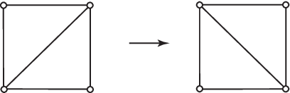
In general, given a representation $\rho\kern-3.0pt:\mathcal{T}_{\lambda}^{q}\to\mathrm{End}(V)$ and another ideal triangulation $\lambda^{\prime}$, it is not easy to decide when the representation $\rho\circ\Phi_{\lambda\lambda^{\prime}}^{q}\kern-3.0pt:\mathcal{T}_{\lambda^{\prime}}^{q}\to\mathrm{End}(V)$ makes sense. This is relatively simple when $\lambda$ and $\lambda^{\prime}$ differ only by one edge, as in Figure 1. We then say that $\lambda$ and $\lambda^{\prime}$ differ by a diagonal exchange. The diagonal exchange is embedded when the four sides of the square where the diagonal exchange takes place are distinct, namely when there are no outside gluings between these sides.

This is a relatively simple consequence of the formula for the coordinate change isomorphism $\Phi_{\lambda\lambda^{\prime}}^{q}$ for a diagonal exchange. With significantly more work to control the invertibility of the images of denominators, it can be extended to the case where $\lambda$ and $\lambda^{\prime}$ can be connected by a sequence of diagonal exchanges.

From now on, we will identify $S$ with the complement $\widehat{\mathbb{C}}-\{v_{1},v_{2},\dots,v_{r}\}$ of $r$ distinct points $v_{1}$, $v_{2}$, …$v_{r}$ in the Riemann sphere $\widehat{\mathbb{C}}=\mathbb{C}\cup\{\infty\}$. Namely, we choose a conformal structure on $S$.

An ideal triangulation $\lambda$ is simple if every edge of $\lambda$ joins two distinct punctures of $S$.

The conformal structure of $S$ then defines a system on complex edge weights on $\lambda$ defined as follows. Choose an arbitrary orientation for the edge $\lambda_{i}$, so that it goes from the puncture $v_{-}$ to the puncture $v_{+}\in\widehat{\mathbb{C}}$. Let $T_{\mathrm{left}}$ and $T_{\mathrm{right}}$ be the two faces of $\lambda$ containing $\lambda_{i}$ and respectively located to the left and to the right of $\lambda_{i}$ for the orientation specified, and let $v_{\mathrm{left}}$ and $v_{\mathrm{right}}$ be the vertices of these two triangles that are different from $v_{-}$ and $v_{+}$. See Figure 1. Then, the weight $x_{i}\in\mathbb{C}^{*}$ is defined as the cross-ratio

In the case of a diagonal exchange, an elementary computation provides:

Note the similarity with the formulas of Proposition 3.

In the same way, around a puncture:

We can use these edge weights $x_{i}$ to construct representations of the Chekhov-Fock algebras attached to simple ideal triangulations of the punctured sphere $S=\widehat{\mathbb{C}}-\{v_{1},v_{2},\dots,v_{r}\}$.

For each puncture $v_{i}$, choose an $N$–root of unity $p_{j}=q^{2n_{j}}$. Then choose a square root $h=\sqrt[2]{p_{1}p_{2}\dots p_{r}}$. If $\lambda$ is a simple ideal triangulation of $S$, Theorem 2 and Lemma 6 then provide an irreducible representation $\rho\kern-3.0pt:\mathcal{T}_{\lambda}^{q}\to\mathrm{End}(V)$, associated to the cross-ratio edge weights $x_{i}$, the $N$–roots $p_{j}$ and the square root $h$.

If we combine Proposition 3, Proposition 4 and Lemma 5, we then obtain:

In order to apply Lemma 7, we will restrict the type of ideal triangulations that we consider.

An example of an ideal cell decomposition is provided by a convex polyhedron $C$ with $r$ vertices in $\mathbb{R}^{3}$. If we choose a homeomorphism between $S$ and the complement of the vertices in the boundary $\partial C$, the pre-images of the edges of $C$ form an ideal cell decomposition of $S$. A famous theorem of Steinitz (see for instance [10]) asserts that an ideal cell decomposition is obtained in this way if and only if each edge of $\lambda$ joins different punctures, if no two distinct edges join the same punctures, and if there is no curve in $S$ which cuts $\lambda$ in exactly two points contained in different edges.

An ideal cell decomposition $\lambda$ of $S$ satisfies the Rivin Condition, or is a Rivin cell decomposition, if it comes from a convex polyhedron $C$ which, in addition, is inscribed in the sphere $\mathbb{S}^{2}$. More precisely, $\lambda$ satisfies the Rivin condition if there exists $v_{1}$, $v_{2}$, …, $v_{r}\in\mathbb{S}^{2}$ and a homeomorphism between $S$ and $\partial C-\{v_{1},v_{2},\dots v_{r}\}$, where $C$ is the convex hull of $\{v_{1},v_{2},\dots v_{r}\}$ in $\mathbb{R}^{3}$, for which $\lambda$ corresponds to the edges of the polyhedron $C$. We will allow the case where the points $v_{1}$, $v_{2}$, …, $v_{r}$ are coplanar, in which case the convex hull $C$ is a flat polygon, and $\lambda$ consists of a chain of $r$ edges subdividing $S$ into two ideal $r$–gons.

From our point of view, a fundamental property of Rivin cell decompositions is that they are simple, in the sense that each edge joins two distinct punctures of $S$.

Igor Rivin [16, 17, 18, 19] (see also [9]) showed that the Rivin condition is equivalent to the existence of a system of real weights on the edges of $\lambda$ satisfying a certain number of linear equalities and inequalities. In particular, for a given ideal cell decomposition, the validity of this property can be decided by a linear programming algorithm. The simplest example of an ideal triangulation that does not satisfies the Rivin Condition is provided by the convex polyhedron obtained by gluing a triangular pyramid with low height on each of the faces of a tetrahedron. The corresponding ideal triangulation of the 6–times punctured sphere is by construction realized by a convex polyhedron, but can be shown to be irrealizable by a convex polyhedron inscribed in the sphere.

When $r=4$, any Rivin triangulation is combinatorially equivalent to a tetrahedron, with three edges arriving at each puncture. In this case, the convex hull becomes flat as one crosses the codimension 1 sratum. The same proof then shows that any two Rivin triangulations of the 4–times punctured sphere can be joined by a sequence of double diagonal exchanges illustrated in Figure 2.

Note that in a double diagonal exchange, the intermediate ideal triangulation is not a Rivin triangulation, but is nevertheless simple. Therefore:

Note that the case where $r=3$ is particularly trivial, since in this case $S$ admits only one Rivin triangulation, decomposing $S$ into two triangles.

We can now put everything together. We fix a conformal structure on the punctured sphere $S$, namely an identification between $S$ and the complement $\widehat{\mathbb{C}}-\{v_{1},v_{2},\dots,v_{r}\}$ of $r$ points in the Riemann sphere $\widehat{\mathbb{C}}$.

After this geometric data, let us choose some algebraic (or number-theoretic) data. We take a root of unity $q$ such that $-q$ is a primitive $N$–root of $(-1)$. Choose an $N$–root of unity $p_{j}=q^{2n_{j}}$ for each puncture of $S$, and a square root $h=\sqrt[2]{p_{1}p_{2}\dots p_{r}}$.

Now, pick a Rivin triangulation $\lambda$ of $S$. The points $v_{i}$ associate a cross-ratio weight $x_{i}\in\mathbb{C}^{*}$ to each edge of $\lambda$. As in §3, the edge weights $x_{i}$, the $N$–roots $p_{j}$ and the square root $h$ define, up to isomorphism, an irreducible representation $\rho_{\lambda}\kern-3.0pt:\mathcal{T}_{\lambda}^{q}\to\mathrm{End}(V)$ of the Chekhov-Fock algebra of $\lambda$.

Consider a diffeomorphism $\varphi\kern-3.0pt:S\to S$, and the ideal triangulation $\varphi(\lambda)$. Combining Lemmas 7, 8 and 9, the representation $\rho\circ\Phi_{\lambda\varphi(\lambda)}^{q}\kern-3.0pt:\mathcal{T}_{\varphi(\lambda)}^{q}\to\mathrm{End}(V)$ makes sense. By Proposition 3 and Lemma 5, this representation $\rho\circ\Phi_{\lambda\varphi(\lambda)}^{q}$ is classified by the cross-ratio edge weights associated to the edges of $\varphi(\lambda)$ by the points $v_{1}$, $v_{2}$, …$v_{r}\in\widehat{\mathbb{C}}$, plus the same puncture weights $p_{j}$ and the same global charge $h$ as $\rho$.

There is also a simpler way to obtain a representation of $\mathcal{T}_{\varphi(\lambda)}^{q}$ from $\rho$. Indeed, $\varphi$ provides a natural isomorphism $I_{\lambda,\varphi}\kern-3.0pt:\mathcal{T}_{\varphi(\lambda)}^{q}\to\mathcal{T}_{\lambda}^{q}$, which sends the generator associated to an edge of $\varphi(\lambda)$ to the generator associated to the corresponding edge of $\lambda$. The representation $\rho\circ I_{\lambda,\varphi}\kern-3.0pt:\mathcal{T}_{\varphi(\lambda)}^{q}\to\mathrm{End}(V)$ is classified by assigning to each edge of $\varphi(\lambda)$ the cross-ratio weight of the corresponding edge of $\lambda$, by assigning to each puncture the puncture weight $p_{j}$ associated by $\rho$ to the preimage of this puncture under $\varphi$, and by the same global charge $h$ as $\rho$.

Now, suppose in addition that $\varphi$ fixes every puncture of $S$. Then each edge of $\lambda$ has the same cross-ratio weight as its image under $\varphi$, since the corresponding cross-ratios involve the same points. Also, $\rho\circ\Phi_{\lambda\varphi(\lambda)}^{q}$ and $\rho\circ I_{\lambda,\varphi}$ then assign the same weight $p_{j}$ to each puncture, and have the same global charge $h$. It follows that the representations $\rho\circ\Phi_{\lambda\varphi(\lambda)}^{q}$ and $\rho\circ I_{\lambda,\varphi}$ are isomorphic.

This means that there is an isomorphism $L_{\varphi}\kern-3.0pt:V\to V$ such that

for every $X\in\mathcal{T}_{\varphi(\lambda)}^{q}$.

It may be more convenient to rewrite this property with the following definition. If $L\kern-3.0pt:W\to W^{\prime}$ is a linear isomorphism between vector spaces, its adjoint homomorphism $\mathrm{Ad}_{L}\kern-3.0pt:\mathrm{End}(W)\to\mathrm{End}(W^{\prime})$ is defined by the property that $\mathrm{Ad}_{L}(A)=L\circ A\circ L^{-1}$. Then the above property can be rewritten as

The isomorphism $L_{\varphi}$ is not unique since multiplying it by a constant does not change the adjoint homomorphism $\mathrm{Ad}_{L_{\varphi}}$. However, because the representation $\rho\circ I_{\lambda,\varphi}$ is irreducible, this is the only ambiguity and $L_{\varphi}$ is unique up to rescaling. In particular, the projective isomorphism $\mathbb{P}L_{\varphi}\kern-3.0pt:\mathbb{P}(V)\to\mathbb{P}(V)$ of the projective space of $V$ is uniquely determined.

Recall from Theorem 2 that the dimension of $V$ is equal to $N^{r-3}$. We can consequently identity $\mathbb{P}(V)$ to the complex projective space $\mathbb{CP}^{N^{r-3}-1}$.

References

- [1] Hua Bai, A uniqueness property for the quantization of Teichmüller spaces, Geom. Dedicata 128 (2007), 1–16.
- [2] Hua Bai, Francis Bonahon, Xiaobo Liu, Local representations of the quantum Teichmüller space, preprint, 2007, (arXiv:0707.2151v1).
- [3] Francis Bonahon, Xiaobo Liu, Representations of the quantum Teichmüller space and invariants of surface diffeomorphisms, Geom. Topol. 11 (2007), 889-938.
- [4] Leonid O. Chekhov, Vladimir V. Fock, Observables in 3D gravity and geodesic algebras, in: Quantum groups and integrable systems (Prague, 2000), Czechoslovak J. Phys. 50 (2000), 1201–1208.
- [5] Paul M. Cohn, Skew Fields: Theory of General Division Rings, Encyclopedia of Mathematics and its Applications 57, Cambridge University Press, 1995.
- [6] Oliver T. Dasbach, Xiao-Song Lin, A volumish theorem for the Jones polynomial of alternating knots, Pacific J. Math. 231 (2007), 279–291.
- [7] Vladimir V. Fock, Dual Teichmüller spaces, preprint, 1997 (ArXiv: Math/dg-ga/9702018)
- [8] Vladimir V. Fok, Leonid O. Chekhov, Quantum Teichmüller spaces (Russian) Teoret. Mat. Fiz. 120 (1999), 511–528; english translation in Theoret. and Math. Phys. 120 (1999), 1245–1259.
- [9] François Guéritaud, On an elementary proof of Rivin’s characterization of convex ideal hyperbolic polyhedra by their dihedral angles, Geom. Dedicata 108 (2004), 111–124.
- [10] Branko Grünbaum, Convex polytopes, Second edition (Volker Kaibel, Victor Klee, Günter M. Ziegler eds.), Graduate Texts in Mathematics 221, Springer-Verlag, New York, 2003.
- [11] Rinat Kashaev, The hyperbolic volume of knots from the quantum dilogarithm, Lett. Math. Phys. 39 (1997), 269–275.
- [12] Rinat Kashaev, Quantization of Teichmüller spaces and the quantum dilogarithm, Lett. Math. Phys. 43 (1998), 105–115.
- [13] Xiaobo Liu, The quantum Teichmüller space as a non-commutative algebraic object, preprint, 2004 (ArXiv:math.GT/0408361).
- [14] Xiaobo Liu, Quantum hyperbolic invariants for diffeomorphisms of small surfaces, preprint, 2005 (ArXiv:math.GT/0603467).
- [15] Hitoshi Murakami, Jun Murakami, The colored Jones polynomials and the simplicial volume of a knot, Acta Math. 186 (2001), 85–104.
- [16] Igor Rivin, On geometry of convex ideal polyhedra in hyperbolic -space, Topology 32 (1993), 87–92.
- [17] Igor Rivin, Euclidean structures on simplicial surfaces and hyperbolic volume, Ann. of Math. 139 (1994), 553–580.
- [18] Igor Rivin, A characterization of ideal polyhedra in hyperbolic -space, Ann. of Math. 143 (1996), 51–70.
- [19] Igor Rivin, Combinatorial optimization in geometry, Adv. in Appl. Math. 31 (2003), 242–271.