The relic density of shadow dark matter candidates

It is almost universally accepted that the picture of the Universe made up of approximately $4\%$ baryonic matter, $23\%$ dark matter and $73\%$ dark energy represents a realistic cosmological model. However, it is astounding that almost $96\%$ of the energy density of the Universe resides in some as-yet-unknown form. What is “dark matter”? What is “dark energy”?

In Refs. [1, 2], a model of dark energy and dark matter was proposed in which a new unbroken gauge group $\mathrm{SU}(2)_{Z}$ – the shadow sector – grows strong at a scale $\sim 10^{-3}\,$eV. The gauge group $\mathrm{SU}(2)_{Z}$ was nicknamed Quantum Zophodynamics, or QZD, in Refs. [1, 2], where the subscript “Z” stands for the Greek word Zophos, meaning darkness. The model is described by an $\mathrm{SU}(2)_{Z}$ instanton-induced potential of an axion-like particle, $a_{Z}$, which possesses two degenerate minima. The degeneracy is lifted by a mechanism described in Refs. [2, 3], yielding a false vacuum with energy density $\sim(10^{-3}\,\text{eV})^{4}$ and a true vacuum with vanishing energy density. The present Universe is assumed to be trapped in the false vacuum [4], whose energy density mimics the cosmological constant. This is, in a nutshell, the dark energy model proposed in Ref. [2], which also computed various quantities of interest such as the tunneling rate to the true vacuum, etc. A Grand Unified Theory (GUT) involving the SM and $\mathrm{SU}(2)_{Z}$ was considered by Ref. [5] (The models presented in Refs. [2, 5] were later revisited by Refs. [6].).

The particle content of the model includes two shadow fermions, $\psi_{\left({L,R}\right),i}^{\left(Z\right)}$ with $i=1,2$, which transform as $\left({1,1,0,3}\right)$ under $\mathrm{SU}(3)_{c}\otimes\mathrm{SU}(2)_{L}\otimes\mathrm{U}(1)_{Y}\otimes\mathrm{SU}(2)_{Z}$, two messenger scalar fields (mediating between the QZD and SM matters; one of which is much heavier than the other [2]) $\tilde{\bm{\varphi}}_{i}^{\left(Z\right)}$ with $i=1,2$ transforming as $\left({1,2,Y_{\tilde{\varphi}}=-1,3}\right)$, and one singlet complex scalar field $\phi_{Z}=\left({1,1,0,1}\right)$ whose imaginary part plays the role of the axion-like particle mentioned above.

As discussed in Ref. [2], the masses of the $\mathrm{SU}(2)_{Z}$ triplet shadow fermions are found to be of the order of 100 - 200 GeV for the $\mathrm{SU}(2)_{Z}$ gauge coupling to grow strong at a scale $\sim 10^{-3}$ eV, needed for the dark energy scenario. This coupling constant starts out at GUT-scale energy with a value comparable to that of the electroweak couplings, remains relatively flat until an energy comparable to the shadow fermion masses is reached, and then starts to grow after the shadow fermions drop out of the Renormalization Group (RG) equations. At that dropout point, the $\mathrm{SU}(2)_{Z}$ gauge coupling becomes comparable to the weak $\mathrm{SU}(2)_{L}$ coupling at the electroweak scale energy. These features have interesting consequences concerning the possibility of the shadow fermions being candidates for cold dark matter (CDM) in the form of weakly interacting massive particles (WIMP’s) ¹¹ 1 For a review on various features of CDM and WIMP, see, e.g., Refs. [7].. The main reason is the fact that the annihilation cross sections for two shadow fermions into two $\mathrm{SU}(2)_{Z}$ “shadow gluons” are of the order of the weak cross sections, a typical requirement for WIMP’s. The estimates that were made in Ref. [2] showed that it was possible for shadow fermions to be candidates for CDM with the right relic density.

In this work, we would like to investigate this scenario in more details and by solving shadow fermions’ evolution equations to determine the conditions under which they can be considered to be WIMP cold dark matter candidates. It will be seen that the mass range for the shadow fermions obtained by the requirement of having the right density fits in snugly with that used in the RG equations (i.e., the $\mathrm{SU}(2)_{Z}$ gauge coupling grows strong at a scale $\sim 10^{-3}$ eV).

The outline of the paper is as follows. First, we go over the QZD model as far as the issue of dark matter is concerned. Then, we derive the evolution equations for shadow fermions and consequently solve them numerically, to obtain their relic density. Finally, the results of our relic density calculations will be presented and discussed, in comparison with the observational values. The shadow fermions relic density, when computed, would only depend on their masses. Therefore, the parameter space is simply two dimensional.

In this work, we only concentrate on the potential candidates for cold dark matter that QZD provides in the form of fermions. However, as discussed in Refs. [1, 2], the model offers a mechanism for leptogenesis through the decay of a messenger field, resulting in a net SM lepton surplus.

For clarity, we list the particle content that is useful for our calculations, in particular the transformation of these particles under $\mathrm{SU}(3)_{c}\otimes\mathrm{SU}(2)_{L}\otimes\mathrm{U}(1)_{Y}\otimes\mathrm{SU}(2)_{Z}$.

• •

  Two shadow fermions $\psi_{\left({L,R}\right),i}^{\left(Z\right)}$ with $i=1,2$, which transform as $\left({1,1,0,3}\right)$.

• •

  Two messenger scalar fields $\tilde{\bm{\varphi}}_{i}^{\left(Z\right)}$, with $i=1,2$, transforming as $\left({1,2,Y_{\tilde{\varphi}}=-1,3}\right)$. For relic density calculations, only the one with mass $\mathcal{O}(<1\,\text{TeV})$, i.e., $\tilde{\bm{\varphi}}_{1}^{\left(Z\right)}$, plays a role while the very heavy one with GUT-scale mass, i.e., $\tilde{\bm{\varphi}}_{2}^{\left(Z\right)}$, is only useful for leptogenesis in this picture [8].

• •

  One singlet complex scalar field $\phi_{Z}=\left({1,1,0,1}\right)$. The imaginary part $a_{Z}$ plays the role of the axion-like particle mentioned in section I. The real part, $\sigma_{Z}$, was used as the inflaton in a model of “low-scale” inflationary universe [9].

We now briefly review the relevant aspects of the shadow sector that would be used in our relic density calculations for shadow fermions.

The standard Boltzmann equation [10] describing the evolution of the number density $n$ of a particle species $\psi$, is

where $H$ is the Hubble parameter, $n_{\mathrm{eq}}$ is the equilibrium density, $v$ is the relative velocity in the annihilation process $\psi\bar{\psi}\to{\text{all}}$, and $\left\langle{\sigma v}\right\rangle$ denotes the thermal averaging of $\sigma v$, with $\sigma$ being the total cross section of the annihilation reaction. The equilibrium density $n_{\text{eq}}$ is given by

where $g$ is the species internal degrees of freedom and $f\left({{\mathbf{x}},{\mathbf{p}}}\right)$ is the equilibrium distribution function. For particles that may play the role of CDM, the equilibrium number density in the nonrelativistic approximation is

where $T$ is the temperature, and $m$ is the mass of the relic. The number density $n$ satisfying Eq. (4) has two behaviors. In early times, $n$ closely follows $n_{\mathrm{eq}}$ but later when the temperature drops below $m$, the mass of the species, $n_{\mathrm{eq}}$ starts to decrease exponentially until a“freeze-out” temperature is reached where the annihilation rate is not fast enough to maintain equilibrium. Below this temperature, $n$ deviates substantially from $n_{\mathrm{eq}}$ and eventually gives the present day abundance of the species. Equation (4) can be solved numerically in relativistic (hot relic) or nonrelativistic (cold relic) regime. Ref. [11] showed that the validity of Eq. (4) and its solution breaks down if the relic particle is the lightest of a set of particles whose masses are near-degenerate and can contribute to the density of the relic through annihilation or decay processes, the so-called coannihilation case.

For QZD’s cold dark matter candidates, both shadow fermions can have present day abundances, if they have similar masses, which blocks the decay channel. For that reason, the evolution equations for the number densities of both species ought to be considered. The trivial reduction of shadow fermions occurs through their annihilations into QZD gauge bosons and the decay of the heavier one. Parallel to that, shadow fermions can annihilate into each other as well, which is analogous to the coannihilation case of Ref. [11].

To summarize, the reactions entering into Boltzmann equations for densities of shadow fermions are

• •

  Annihilation of shadow fermions into shadow gluons: $\psi_{i}^{\left(Z\right)}\bar{\psi}_{i}^{\left(Z\right)}\rightleftarrows\bm{A}^{\left({Z}\right)}\bm{A}^{\left({Z}\right)}$

• •

  Annihilation of a pair of one species into a pair of another: $\psi_{1}^{\left(Z\right)}\bar{\psi}_{1}^{\left(Z\right)}\rightleftarrows\psi_{2}^{\left(Z\right)}\bar{\psi}_{2}^{\left(Z\right)}$.

• •

  The decay of the heavier one into the lighter one and SM leptons: $\psi_{2}^{\left(Z\right)}\rightarrow l\bar{l^{\prime}}\psi_{1}^{\left(Z\right)}$.

We assume negligible chemical potential for shadow fermions, which implies symmetry among the number densities for particle and antiparticle of each species. To be inclusive, there can be a particle-antiparticle asymmetry in the shadow sector originating from the decay mechanism of messenger fields. The decay of messenger fields induces a particle-antiparticle asymmetry in SM leptons (see the decay of a messenger boson in Fig. 11). The corresponding asymmetry in the shadow sector is expected to be as small as $\mathcal{O}\left({10^{-7}}\right)$ and therefore negligible to be considered in our relic density calculations.

The evolution equations for number densities $n_{1}$, $n_{2}$ of shadow fermions $\psi_{1}^{(Z)}$, $\psi_{2}^{(Z)}$ are in the form

where $\Gamma_{21}$ is the decay rate of the heavier shadow fermion, i.e., $\psi_{2}^{\left(Z\right)}$, $\sigma_{ij}$ (with $i,j=1,2,A$) refers to the total annihilation cross section for the processes

and $v_{ij}$ is the relative velocity of the annihilating particles for each reaction. Also, with a Maxwell-Boltzmann distribution function²² 2 It has been shown that the use of correct statistics would only amount to less than 1% difference (see Ref. [12])., $n_{i,{\text{eq}}}$ is given by

where $T_{Z}$ is the temperature of QZD matter, $m_{i}$ is the mass of the species and $K_{2}$ is the modified Bessel function of second kind. The ${1\mathord{\left/{\vphantom{12}}\right.\kern-1.2pt}2}$ factor on the right hand side of Eqs. (6) is to account for non-identical annihilating shadow fermions.

Equations  (6) can be written in a more convenient form by considering the number of particles in a comoving volume

which is the ratio of number density to entropy density, with the time derivative in the form

In the absence of entropy production (i.e., $s={S\mathord{\left/{\vphantom{S{R^{3}}}}\right.\kern-1.2pt}{R^{3}}}$ with $S=\mathrm{const.}$)

which results in

The evolution equations, then, can be reformulated in the form

where $Y_{i,\text{eq}}=n_{i,\text{eq}}/s$. Additionally, it is convenient to use the QZD plasma temperature $T_{Z}$ as independent variable, in place of time $t$. The relation between $T$ (the photon temperature) and $T_{Z}$ is easily found by the entropy conservation [1, 2]. The technique is essentially the same as that for finding the neutrino temperature using entropy conservation [10]. For example, at temperatures higher than the mass of the lighter messenger field (i.e., $\tilde{\bm{\varphi}}_{1}^{\left(Z\right)}$) $T>m_{\varphi_{1}}$, the QZD matter is in thermal equilibrium with the rest of the Universe, i.e., $T_{Z}=T$. When $T$ falls below the mass of the lighter messenger field, $T<m_{\varphi_{1}}$, the QZD plasma conserves its own entropy separately and maintains its own temperature $T_{Z}\neq T$. The relation between $T$ and $T_{Z}$ from there on can be found by entropy conservation anytime a particle decouples and transfers its entropy to the relativistic matter. At present, i.e., after $e^{\pm}$ decoupling, $T_{Z}=\left[{{{\left({{{43}\mathord{\left/{\vphantom{{43}{583}}}\right.\kern-1.2pt}{583}}}\right)}\mathord{\left/{\vphantom{{\left({{{43}\mathord{\left/{\vphantom{{43}{583}}}\right.\kern-1.2pt}{583}}}\right)}{\left({{4\mathord{\left/{\vphantom{11{18}}}\right.\kern-1.2pt}{18}}}\right)}}}\right.\kern-1.2pt}{\left({{11\mathord{\left/{\vphantom{11{18}}}\right.\kern-1.2pt}{18}}}\right)}}}\right]^{{1\mathord{\left/{\vphantom{113}}\right.\kern-1.2pt}3}}T$. Ref. [1, 2] discusses the relation between $T_{Z}$ and $T$ in more detail. Let us define $x_{i}={{m_{i}}\mathord{\left/{\vphantom{{m_{i}}{T_{Z}}}}\right.\kern-1.2pt}{T_{Z}}}$, we have

where the time derivative of $T_{Z}$ satisfies

Considering all this, we can rewrite Eqs. (14) in their final forms

Equations (17) are first-order coupled differential equations in the form of Riccati equation, which ought to be solved numerically. The integration of Eqs. (17) from early Universe to present $T_{Z}^{0}=1.346$ K (corresponding to photon temperature $T=2.725$ K) yields today’s number densities $Y_{i}^{0}$. The present-day relic density of shadow fermion $\psi_{i}^{\left({Z}\right)}$ in units of critical density $\rho_{\text{crit}}$ is then

where $s_{0}$ is the present-day entropy density of the shadow sector and $\rho_{\text{crit}}=3H_{0}^{2}/8\pi G$. Finally, with $H_{0}=100h$ $\text{km}~\text{sec}^{-1}~\text{Mpc}^{-1}$ and $s_{0}=12\pi^{2}T_{Z}^{0\,3}/45$, Eq. (18) can be written in the from

where $h$ is the Hubble constant in units of 100 $\text{km}~\text{sec}^{-1}~\text{Mpc}^{-1}$. Since $\psi_{2}^{\left({Z}\right)}$ decays, the relevant relic density is that of $\psi_{1}^{\left({Z}\right)}$. If $m_{1}=m_{2}$, however, both shadow fermions can have present day abundances and only in such case, may we speak of two relic densities.

Equations (17) include thermal averages $\langle{\sigma v}\rangle$’s, Hubble parameter $H$, and the derivative of entropy density ${{ds}\mathord{\left/{\vphantom{{ds}{dx_{i}}}}\right.\kern-1.2pt}{dx_{i}}}$, all of which need to be determined for numerical integration.

The annihilation cross sections and the decay rate $\Gamma_{21}$ can be calculated analytically. They are derived in Appendixes  A and B and are given in closed forms, to leading order. The thermal averages $\langle{\sigma v}\rangle$’s were then computed numerically using the compact integral form of Ref. [13]. In Appendix C, the relativistic thermal averages are provided in closed integral forms, expressed in terms of $x_{i}$.

On the other hand, the Hubble parameter in a radiation-dominated Universe is given by

where $G$ is the gravitational constant and $\rho$ is the total energy density of the Universe, written as

where $g_{\text{eff}}\left(T\right)$ is the effective number of relativistic degrees of freedom. Ref. [13] provides $g_{\text{eff}}\left(T\right)$ values for two QCD phase transition temperatures $T_{\text{QCD}}=150$ and 400 MeV. We made use of the $g_{\text{eff}}\left(T\right)$ values corresponding to $T_{\text{QCD}}=150$ MeV, which is a smoother function, as opposed to $T_{\text{QCD}}=400$ MeV. It turns out that the solutions to Eqs. (17) do not depend on the choice of $T_{\text{QCD}}$, mainly because the freeze-out temperatures for shadow fermions are always much higher than $T_{\text{QCD}}$, due to their large masses. As we already discussed, the relation between $T$ and $T_{Z}$ can be easily determined by entropy conservation. As a result, the Hubble parameter in evolution equations was evaluated in terms of $T_{Z}$ and consequently $x_{i}$, consistently.

The entropy density $s$ , in Eqs. (17), is mostly the entropy of the shadow sector. For temperatures $T>m_{\varphi_{1}}$, the QZD matter is in thermal equilibrium with normal matter and $s$ is

where $g_{\ast s}={{459}\mathord{\left/{\vphantom{{459}{4}}}\right.\kern-1.2pt}{4}}$, and $T=T_{Z}$. However, for most of the time $T<m_{\varphi_{1}}$ and $s$ is the entropy of the shadow sector, which is conserved separately, given by

In both cases $s$ is easily evaluated in terms of $x_{i}$, providing values for ${{ds}\mathord{\left/{\vphantom{{ds}{dx_{i}}}}\right.\kern-1.2pt}{dx_{i}}}$ of Eqs. (17).

The numerical integration of the density evolution equations, Eqs. (17), was carried out using an implicit trapezoidal scheme³³ 3 We implemented the idea of the backward differentiation formulas adapted to implicit trapezoidal scheme, presented in Ref. [14], for a system of Riccati equations.. We integrate from $x_{i}=0$ to $x_{i}=m_{i}/T_{Z}^{0}$, where $T_{Z}^{0}=1.346$ K is the present-day temperature of the QZD matter corresponding to $T_{0}=2.725$ K, the photon temperature of the Universe today.

Equations (17) were integrated for different sets of masses of shadow fermions varying between 30 and 300 GeV. The QZD coupling constant, $\alpha_{Z}\left({E}\right)$, values at energies $\Lambda_{Z}<E<10^{23}\text{ GeV}$ are given for different sets of $m_{1}$ and $m_{2}$ in Ref. [2]. Within the mass range we perform our relic density calculations, $\alpha_{Z}$ varies so slowly and continuously that it can be obtained for any set of $m_{1}$ and $m_{2}$ by simple interpolation and extrapolation of the values provided in Ref. [2]. In this work, we have taken $\alpha_{Z}$ dependence on $m_{1}$, $m_{2}$, and $E$ into account in our relic density calculations. Nevertheless, it is worth mentioning that for a fixed $m_{2}$ and at a given $E$, $\alpha_{Z}$ does not vary much as $m_{1}$ changes. For example, from Figs. (1-3) of Ref. [2], for $m_{2}=$ 100 GeV and at $E=$ 150 GeV one obtains

which demonstrate how $\alpha_{Z}$ varies for $1{\text{ GeV}}\leqslant m_{1}\leqslant 50{\text{ GeV}}$ . The $\alpha_{Z}$ variation within such range (and similar $m_{1}$ ranges) is even less noticeable in relic density calculations, since we are dealing with $\alpha_{Z}^{2}$ in the annihilation cross sections. Our calculations showed that one could safely use an average $\alpha_{Z}^{2}$ value over a wide range of $m_{1}$ values without any sensible loss of accuracy. For instance, an $\alpha_{Z}^{2}=3.49961\times 10^{-2}$ for the above range works just fine.

Ref. [2] carries out RG analysis of QZD’s coupling constant considering a messenger field mass scale (mass of $\tilde{\bm{\varphi}}_{1}^{\left(Z\right)}$ the lighter messenger field) $m_{\varphi_{1}}=300$ GeV and higher, which points to when the QZD plasma decouples from the rest of the Universe. For our relic density calculations, we always chose $m_{\varphi_{1}}>m_{2}$. It turns out that the relic density of shadow fermions does not depend on the choice of $m_{\varphi_{1}}>m_{2}$, as long as they are sufficiently apart⁴⁴ 4 The thermal contact between the shadow and visible sectors may still be in effect through virtual exchange of a messenger boson for some temperatures below the mass of the lighter messenger field. With $m_{\varphi_{1}}$ being sufficiently larger than $m_{2}$, the QZD plasma is ensured to have decoupled from the rest of the Universe before $\psi_{2}^{\left(Z\right)}$ enters its nonrelativistic epoch, decoupling from an isolated QZD matter.. That is mainly because the relic densities of shadow fermions (or more generally WIMP’s) are mostly determined in their nonrelativistic epoch, i.e., for our case when $T_{Z}\leq m_{2}$.

The decay of $\psi_{2}^{\left({Z}\right)}$ into a pair of SM leptons and $\psi_{1}^{\left({Z}\right)}$ happens through a messenger field (see Fig. 11 of Appendix B). When the mass difference $\Delta m=m_{2}-m_{1}$ is not very large, the decay rate for one of the possible decays can be given in an approximate form

where $\alpha_{\varphi_{1}}=g^{2}_{\varphi_{1}}/4\pi$, $\Gamma_{\varphi_{1}}$ is the decay width of the messenger field and $x=m_{1}^{2}/m_{2}^{2}$. As already said, we concentrate on the messenger field being sufficiently heavier than $\psi_{2}^{\left({Z}\right)}$ where the “singularity” in the decay rate is not present, which can be seen from the approximate from of $\Gamma_{21}$, Eq. (27). We shall explain the interesting case of $m_{2}=m_{\varphi_{1}}$ when we present our results in the next section. It is worth mentioning, nevertheless, that such mass degeneracy poses no computational difficulty due to the presence of the messenger field’s decay width $\Gamma_{\varphi_{1}}$.

On the other hand, $\alpha_{\varphi_{1}}$ is constrained for the model to predict the observed baryon asymmetry through an initial lepton asymmetry produced in the decay of messenger fields [2]. That requirement sets $\alpha_{\varphi_{1}}\approx 2.9\times 10^{-17}$, which will consequently correspond to a long lifetime for $\psi_{2}^{\left({Z}\right)}$ (not less than $10^{7}$ sec). For that reason, the decay rate of $\psi_{2}^{\left({Z}\right)}$ does not effectively enter the relic density calculations⁵⁵ 5 That means the decay of $\psi_{2}^{\left({Z}\right)}$ is not determinant of the freeze-out temperatures., where the evolution equations are dominated by the annihilation processes. The remnant $\psi_{2}^{\left({Z}\right)}$’s (after the freeze-out) decay into SM leptons and $\psi_{1}^{\left({Z}\right)}$’s anyway and we end up with no relic for $\psi_{2}^{\left({Z}\right)}$ if the shadow fermion masses are not degenerate.

The relic density of shadow fermions depend on two parameters: their masses, $m_{1}$, and $m_{2}$. The masses affect the annihilation cross sections and consequently the dynamics of the evolution equations. Our relic density calculation results, therefore, are displayed either in terms of masses or mass difference.

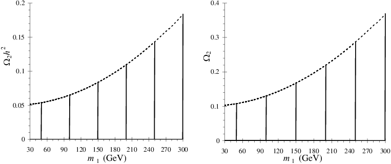
Suppose there were only one shadow fermion; in that case, the corresponding evolution equation would be administered by shadow fermion’s annihilation process and the expansion of the Universe. Since the annihilation cross section into shadow gluons and its thermal average $\left\langle{\sigma v}\right\rangle$ are inversely proportional to the mass squared, a heavier shadow fermion would freeze out earlier than a lighter one, as it could not sustain a rate larger than the Hubble rate for as long. That would allow less time (at temperatures below the mass of the sole shadow fermion) for the Boltzmann factor to diminish the density, which would result in a higher relic density compared to a light shadow fermion’s. This can be seen from the behavior shown by the dashed line in Figs. 1, 2, and 3, which describes the density of $\psi_{1}^{\left({Z}\right)}$ or $\psi_{2}^{\left({Z}\right)}$ if they were the sole fermion in the QZD particle content. From those graphs, one sees that a heavy sole shadow fermion would have a higher relic than a light one.

With two shadow fermions, however, there are two mechanisms governing the evolution equations, besides the effect of the expanding Universe. There are those reactions, which exhaust the phase space from the species and those that populate it. The evolution of the number densities is determined by the competition of those mechanisms. The outcome of such a competition, on the other hand, depends on the masses of shadow fermions.

Of those mechanisms, the decay of $\psi_{2}^{\left({Z}\right)}$ plays no role in the early dynamics of evolution equations. Briefly, that is because the lifetime of $\psi_{2}^{\left({Z}\right)}$, which depends on $m_{1}$, $m_{2}$, and $m_{\varphi_{1}}$, turns out either too long or too short to be a factor in the determination of freeze-out temperatures. For a well-separated set of $m_{2}$, and $m_{\varphi_{1}}$, the lifetime of $\psi_{2}^{\left({Z}\right)}$ is within $10^{7}{\text{ sec}}\lesssim\tau_{2}\lesssim 10^{13}{\text{ sec}}$ when $m_{1}\neq m_{2}$, i.e, a nondegenerate case. That roughly corresponds to a temperature $1{\text{ keV}}\lesssim T\lesssim 1{\text{ eV}}$, which is well after a typical freeze-out for $\psi_{2}^{\left({Z}\right)}$. That means, the remainder of $\psi_{2}^{\left({Z}\right)}$ will decay into $\psi_{1}^{\left({Z}\right)}$ and SM leptons after the freeze-out, which leaves no present day abundance for $\psi_{2}^{\left({Z}\right)}$. The decay of an unstable shadow fermion at such low temperature into SM leptons can potentially disturb the cosmic microwave background (CMB). That, as we shall see, will place a bound on the mass of $\psi_{2}^{\left({Z}\right)}$ which determines the density of $\psi_{2}^{\left({Z}\right)}$ at the time of its decay. With a mass degeneracy, i.e., $m_{1}=m_{2}$, of course $\psi_{2}^{\left({Z}\right)}$ is stable and decay is irrelevant. In that case, since the annihilation channel into another is also closed, we end up with two one-species cases: one for $\psi_{1}^{\left({Z}\right)}$ and one for $\psi_{2}^{\left({Z}\right)}$.

When $m_{2}=m_{\varphi_{1}}$, the decay width of the messenger field determines the lifetime of $\psi_{2}^{\left({Z}\right)}$. As discussed in Ref. [2], the requirement for the lightest messenger field to decouple before decaying yields $\Gamma_{\varphi_{1}}\approx m_{\varphi_{1}}\alpha_{\varphi_{1}}$, which is less than the expansion rate of the Universe, at $T=m_{\varphi_{1}}$. Since $\alpha_{\varphi_{1}}$ is of the order $\sim 10^{-17}$, a lifetime of $10^{-25}{\text{ sec}}\lesssim\tau_{2}\lesssim 10^{-15}{\text{ sec}}$ for $\psi_{2}^{\left({Z}\right)}$ is obtained. With such short lifetime, $\psi_{2}^{\left({Z}\right)}$ decays well prior to the decoupling of QZD matter, i.e., when QZD and the SM plasmas are in equilibrium. Effectively, that means we are down to the one-species case, regardless of the value of $m_{2}$.

Thus, the annihilation processes and their competition will mainly decide for the early dynamics of the evolution equations. At temperatures above the mass of the heavier shadow fermion $\psi_{2}^{\left({Z}\right)}$, both shadow fermions contribute to the population of another through the annihilation process $\psi_{i}^{\left(Z\right)}\bar{\psi}_{i}^{\left(Z\right)}\to\psi_{j}^{\left(Z\right)}\bar{\psi}_{j}^{\left(Z\right)}$. As temperature decreases, the contribution of the lighter shadow fermion $\psi_{1}^{\left({Z}\right)}$ into the population of $\psi_{2}^{\left({Z}\right)}$ diminishes until it stops at an energy when it is no longer kinematically allowed. From there on, $\psi_{2}^{\left({Z}\right)}$ will lose pairs monotonically due to its annihilations into shadow gluons and $\psi_{1}^{\left({Z}\right)}$ pairs, while $\psi_{1}^{\left({Z}\right)}$ receives pairs from $\psi_{2}^{\left({Z}\right)}$’s annihilation and at the same time loses pairs due to annihilation into shadow gluons.

The annihilation into $\psi_{1}^{\left({Z}\right)}$ provides an additional channel for $\psi_{2}^{\left({Z}\right)}$ to keep up with the expansion rate of the Universe and therefore delay the freeze-out. This reduces the density of $\psi_{2}^{\left({Z}\right)}$ prior to its freeze-out, compared to the one-species case, in two ways: (i) $\psi_{2}^{\left({Z}\right)}$ pairs are lost into $\psi_{1}^{\left({Z}\right)}$ pairs in addition to those lost into shadow gluons, (ii) the Boltzmann factor for temperatures $T_{Z}<m_{2}$ can act on $\psi_{2}^{\left({Z}\right)}$’s density for a longer time.

All this, though, depends on how apart $\psi_{1}^{\left({Z}\right)}$ and $\psi_{2}^{\left({Z}\right)}$ are, masswise, at a fixed $m_{2}$. Since the available phase space for $\psi_{2}^{\left(Z\right)}\bar{\psi}_{2}^{\left(Z\right)}\to\psi_{1}^{\left(Z\right)}\bar{\psi}_{1}^{\left(Z\right)}$ increases with the mass difference $\Delta m=m_{2}-m_{1}$, we expect $\psi_{2}^{\left({Z}\right)}$’s density at freeze-out becoming small for an increasing $\Delta m$ due to a growing annihilation rate. On the other hand, a small mass difference reduces the phase space for the annihilation process and therefore increases the density. Knowing this is important in understanding the constraint on $\psi_{2}^{\left({Z}\right)}$’s density at the time of decay. Since the remaining $\psi_{2}^{\left({Z}\right)}$’s will decay anyway, there will be no relic for $\psi_{2}^{\left({Z}\right)}$ if $m_{1}\neq m_{2}$, which is reflective in Fig. 1, where $\psi_{2}^{\left({Z}\right)}$’s relic densities are displayed in solid lines for different $m_{2}$’s as $m_{1}$ varies. The relic density of $\psi_{2}^{\left({Z}\right)}$ falls down rapidly when the mass difference between the two shadow fermions is enough to allow the decay before our time and therefore to deplete the phase space from $\psi_{2}^{\left({Z}\right)}$ pairs. The maximum relic density, however, is always at $m_{1}=m_{2}$, where the annihilation cross section, $\sigma_{ij}$, and the decay rate $\Gamma_{21}$ are vanishing and it is essentially the one-species case.

The situation for $\psi_{1}^{\left({Z}\right)}$ is more complicated. The relic density of $\psi_{1}^{\left({Z}\right)}$ is shown through a solid line in Figs. 2, and 3 for different $m_{2}$’s as $m_{1}$ varies. For an extremely heavy $\psi_{1}^{\left({Z}\right)}$, i.e. $m_{1}=m_{2}$, $\psi_{1}^{\left({Z}\right)}$’s relic density coincides with the one-species case, as expected. As $\Delta m$ deviates from zero $\psi_{2}^{\left({Z}\right)}$ starts to dispense $\psi_{1}^{\left({Z}\right)}$ pairs into the phase space (by annihilation earlier, and decay later) and thus $\Omega_{1}$ increases. Prior to freeze-out, this positive contribution comes from the pair annihilation of $\psi_{2}^{\left({Z}\right)}$ into $\psi_{1}^{\left({Z}\right)}$, which will face a growing competition from $\psi_{1}^{\left({Z}\right)}$’s annihilation channel into shadow gluons, as $m_{1}$ declines. Since the annihilation cross section into shadow gluons grows for small masses, it will start to contend the rate of the extra $\psi_{1}^{\left({Z}\right)}$ pairs coming from $\psi_{2}^{\left({Z}\right)}$’s annihilation. For that reason, as $m_{1}$ decreases, the annihilation channel into shadow gluons depletes the phase space from $\psi_{1}^{\left({Z}\right)}$ pairs more effectively and therefore $\psi_{1}^{\left({Z}\right)}$’s density before the freeze-out, which consequently diminishes its relic $\Omega_{1}$. After the freeze-out, the remnant of $\psi_{2}^{\left({Z}\right)}$ will decay into $\psi_{1}^{\left({Z}\right)}$ and lifts $\Omega_{1}$, very much by a constant, except at small $\Delta m$’s where $\psi_{2}^{\left({Z}\right)}$’s density is larger.

For a nondegenerate mass case, $\psi_{1}^{\left({Z}\right)}$’s relic density is what remains of shadow fermions. It is only at $m_{1}=m_{2}$ that the relic consists of both shadow fermions (equally so). To be inclusive of the degenerate case, the total relic density of shadow fermions $\Omega_{T}=\Omega_{1}+\Omega_{2}$ is presented in Fig.  4 against both masses and in Figs. 5, 6 against $m_{1}$ at fixed $m_{2}$’s, where the one-species case is also presented. The gray areas in Figs. 5, and 6 indicate the current bounds on the dark matter density from WMAP3 and all data sets [15].

It can be seen in Figs. 5, and 6 that the total relic density $\Omega_{T}$ increases as $m_{1}$ does, attaining a sharp maximum for the degenerate case, as if there were two “one-species” shadow fermions. On the other hand, $\Omega_{T}$ also increases with $m_{2}$, which means for staying in the cosmologically allowed region a larger and larger mass difference would be needed. The two extremes are at $m_{2}=50$ GeV, where the degenerate case is just making it to the allowed region, and $m_{2}=300$ GeV, where a large mass difference is needed to stay relevant.

This can also be seen by looking at Fig. 8, in which the total relic density is displayed versus $\Delta m$ and the bounds are shown with two white dashed lines. We conclude that for $m_{2}<50$ GeV, the total relic density is not enough to account for the total dark matter, even though the shadow fermions would still be relic particles taking on a fraction of the dark matter in the Universe.

On the other hand, for $m_{2}\gtrapprox 320$ GeV, the total density of shadow fermions go beyond the upper bound and give unacceptable values even if we extend the mass difference to an extreme where $m_{1}=1$ GeV. That is shown in Fig. 7, where the total relic density at $m_{2}=318$ GeV is only viable for a large mass difference of about 317 GeV and at $m_{2}=400$ GeV is no longer relevant. By going to such an extreme mass difference, we place a naive bound on the mass of the heavier shadow fermion, i.e., $m_{2}\approxeq 320$ GeV, above which the total relic density is no longer viable.

There are, however, more restrictive bounds on $m_{2}$ coming from the decay of $\psi_{2}^{\left({Z}\right)}$ into SM leptons at low temperature, and its potential disturbance of the CMB of the Universe. We demand that

1. 1.

   The density of $\psi_{2}^{\left({Z}\right)}$ at the time of decay could not exceed that of the SM particles.

2. 2.

   The CMB density disturbance caused by the late decay of $\psi_{2}^{\left({Z}\right)}$ would not violate the CMB fluctuation, which has been observed to be at $10^{-5}$ level [15].

Figure 9 illustrates these two conditions in graphs versus the mass of $\psi_{2}^{\left({Z}\right)}$. In Fig. 9 a, ${{\rho_{2}}\mathord{\left/{\vphantom{{\rho_{2}}{\rho_{{\text{SM}}}}}}\right.\kern-1.2pt}{\rho_{{\text{SM}}}}}$, i.e., the density of $\psi_{2}^{\left({Z}\right)}$ to the density of the SM matter – right before the decay – is plotted, which shows that the density of $\psi_{2}^{\left({Z}\right)}$ remains less than that of the SM particles for $m_{2}\leqslant 285$ GeV. The possible CMB density disturbance, ${{\delta\rho_{\gamma}}\mathord{\left/{\vphantom{{\delta\rho_{\gamma}}{\rho_{\gamma}}}}\right.\kern-1.2pt}{\rho_{\gamma}}}$, that the late decay of $\psi_{2}^{\left(Z\right)}$ can create is shown in Fig. 9 b. The CMB density disturbance goes above the $10^{-5}$ order for $\psi_{2}^{\left(Z\right)}$s heavier than 245 GeV. The two above conditions, therefore, place a strong bound of 245 GeV on $\psi_{2}^{\left(Z\right)}$’s mass.

As we discussed, the lifetime of $\psi_{2}^{\left({Z}\right)}$ could be very short if $\psi_{2}^{\left({Z}\right)}$ and the messenger field were degenerate in mass. In that case, the total relic density of shadow fermions is simply that of the one-species case and it yields the right density for masses between 190 and 210 GeV.

For $50\text{ GeV}\lessapprox m_{2}\lessapprox 245\text{ GeV}$, the total relic density of shadow fermions can account for the amount of the dark matter in the Universe, depending on the mass difference. The total relic density lies within the observational bounds with small and even zero mass difference for light $\psi_{2}^{\left({Z}\right)}$’s and with large mass differences when $\psi_{2}^{\left({Z}\right)}$ is heavy.

We solved evolution equations for number densities of shadow fermions and obtained their total present-day density. The heavier shadow fermion turned out to be long lived if its mass differs from that of the messenger field. In that case, our results revealed an upper bound on the mass of the heavier shadow fermion, i.e., $m_{2}\approx 245$ GeV, above which its late decay can potentially disturb the CMB density of the Universe beyond the measured fluctuation level of $10^{-5}$.

For lighter shadow fermions, the total relic density can account for the entire dark matter of the Universe depending on the mass combination of shadow fermions. When the total density falls short of the observationally suggested density, it still, for most of masses, provides significant fraction of the dark matter of the Universe.

Our results showed that if the heavier shadow fermion’s mass is large, considerable mass differences would be needed to comply with experimental bounds. On the other hand, if the heavier shadow fermion’s mass is small, little or even no mass differences suffice to give the right relic density. In that sense, degenerate and near-degenerate mass cases become relevant at low mass scales, but not for less than 50 GeV.

A very short lifetime is expected for the heavier shadow fermion if its mass is the same as that of the messenger field. In that case, the calculations reduce to a one-species case. Our results suggest that a sole shadow fermion must have a mass of about 190 – 210 GeV to account for the whole dark matter of the Universe.

Last but not least, possible detections of the shadow fermion CDM candidates are briefly discussed in Ref. [2]. Needless to say, more work along this line is warranted for this model.

References

- [1] P. Q. Hung, [arXiv:hep-ph/0504060v2].
- [2] P. Q. Hung, Nucl. Phys. B 747, 55 (2006a), [arXiv:hep-ph/0512282v2].
- [3] P. Q. Hung, [arXiv:0707.2791v1].
- [4] P. Q. Hung, J. Phys. A 40, 6871 (2007b), [arXiv:astro-ph/0612245v1].
- [5] P. Q. Hung and P. Mosconi, [arXiv:hep-ph/0611001v2].
- [6] C. R. Das and L. V. Laperashvili, [arXiv:0712.0253v3]; C. R. Das and L. V. Laperashvili, [arXiv:0712.1326v1].
- [7] G. Jungman, M. Kamionkowski, and K. Griest, Phys. Rept. 267, 195 (1996), [arXiv:hep-ph/9506380v1]; G. Bertone, D. Hooper, and J. Silk, Phys. Rept. 405, 279 (2005), [arXiv:hep-ph/0404175v2].
- [8] P. Q. Hung, [arXiv:hep-ph/0604063v4].
- [9] P. Q. Hung, E. Masso, and G. Zsembinszki, J. Cosmol. Astropart. Phys 2006, 004 (2006), [arXiv:astro-ph/0609777v2].
- [10] E. W. Kolb and M. S. Turner, The Early Universe, vol. 69 of Frontiers in Physics (Addison-Wesley, 1990), ISBN 0-201-11603-0.
- [11] P. Binetruy, G. Girardi, and P. Salati, Nucl. Phys. B 237, 285 (1984); K. Griest and D. Seckel, Phys. Rev. D 43, 3191 (1991).
- [12] R. J. Scherrer and M. S. Turner, Phys. Rev. D 33, 1585 (1986).
- [13] P. Gondolo and G. Gelmini, Nucl. Phys. B 360, 145 (1991).
- [14] L. Dieci, SIAM J. Numer. Anal. 29, 781 (1992).
- [15] D. N. Spergel, R. Bean, O. Doré, M. R. Nolta, C. L. Bennett, J. Dunkley, G. Hinshaw, N. Jarosik, E. Komatsu, L. Page, et al., Astrophys. J. Suppl. 170, 377 (2007), [arXiv:astro-ph/0603449v2].