Coupled map lattices (CMLs) as introduced by Kaneko and Kapral [1, 2] some 24 years ago are a paradigm of spatially extended dynamical systems with discrete evolution in space and time. They exhibit a rich structure of complex dynamical phenomena [3, 4, 5, 6, 7, 8, 9] . Of particular interest are CMLs that exhibit spatio-temporal chaotic behaviour. In certain cases it can be rigorously proved that the system possesses an ergodic invariant measure [10, 11, 12, 13, 14] provided the coupling is small enough. Various interesting aspects of chaotic CMLs have been investigated in [15, 16, 17, 18, 19, 20, 21, 22, 23].

CMLs are not only of theoretical interest in the theory of dynamical systems but they also have applications for a variety of physical problems, e.g. as models for hydrodynamical flows, turbulence, chemical reactions, or synchronization. A very interesting new application in quantum field theories has been pointed out in [5, 24]: Certain types of coupled map lattices can serve as models of vacuum fluctuations. This may at first sight look as a rather exotic type of theory. The remarkable observation, however, is that these types of coupled map lattices seem to distinguish certain numerical values of coupling constants that coincide with those observed in the standard model of electroweak and strong interaction. For more details on this, see [5, 24, 25, 26, 27, 28]. The main idea underlying this approach is that indeed the fundamental constants of nature may be fixed by dynamically evolving chaotic states of vacuum fluctuations that possess the strongest random properties that are possible for a smooth coupled deterministic chaotic system. These types of vacuum fluctuations may underly the currently observed dark energy in the universe [27, 29].

The relevant classes of coupled map lattices for this approach have been termed ‘chaotic strings’ [5, 24]. This is a name only, it should be clear that chaotic strings are very different from ‘ordinary’ strings studied in string theory. Chaotic strings are closely related to an alternative way of quantizing classical systems which is based on the so-called ‘chaotic quantization’ method [25, 30, 31]. Chaotic quantization yields additional sectors of highly nonlinear field theories, which can be used to stabilize the fundamental constants of nature. In theories of quantum gravity standard model parameters are often thought of as being related to certain types of scalar fields, so-called moduli fields [28, 32]. A varying standard model parameter (e.g. the fine structure constant) can be essentially regarded as such a moduli field. These moduli fields evolve to minima of their potentials. In this way for example the fine structure constant stabilizes at its currently observed low-energy value of $1/137.036$. The main idea underlying chaotic quantization methods is that the chaotic string dynamics produces suitable effective potentials for moduli fields which fix and stabilize fundamental constants, avoiding anthropic considerations.

Chaotic strings can occur in different versions, depending on the way the coupling is done. In this paper, we study discrete symmetry transformations for the various possible chaotic string dynamics. From a nonlinear dynamics point of view, chaotic strings are just diffusively or anti-diffusively coupled map lattices consisting locally of positive or negative $N$-th order Tchebyscheff maps $(N\geq 2)$ [5, 22, 23, 33, 34, 35, 36, 37] with either forward or backward coupling. These live on 1-dimensional lattices with periodic boundary conditions. For each $N$ there are a priori 8 different chaotic strings. But we will show that this actually reduces to four different relevant strings if $N$ is even and two different relevant strings if $N$ is odd, due to the fact that there is a number of discrete coordinate transformations which one can use to map one string dynamics into another one. Our paper for the first time investigates these discrete symmetries in a systematic and complete way. In ordinary quantum field theories, it is well known that discrete symmetries such as CPT (charge, parity, time reversal) play an important role. Our paper here investigates the analogue of this for chaotic strings.

Our main examples are chaotic strings build up from Tchebyscheff maps of order $N=2$ and $N=3$, which can be regarded as kind of ‘ground states’ (with even or odd parity) in quantum gravity embeddings of chaotic strings [5]. For the calculation of expectations of observables associated with the chaotic dynamics it is important to know whether the dynamics is ergodic. In fact, non-ergodicity can be related to spontaneous symmetry breaking in this context (a particular attractor out of several is spontaneously chosen, depending on the inital condition). For more details on this symmetry breaking aspect, see [26]. To completely understand the discrete symmetry transformation behaviour of chaotic strings it is thus important to investigate the ergodic properties and the convergence behaviour of observables in the various parameter regions. We will investigate this question numerically and define some suitable measures of homogenity, which test the dependence of expectations of local observables under translations on the lattice and under changes of the initial conditions. An observable of particular interest is the nearest neighbour correlation function, whose zeros were used in [5, 24] to single out distinguished standard model parameters. Our investigation here analyses which of these zeros are in parameter regions with ergodic behaviour and well-defined convergence properties of expectations. Interesting enough, our analysis shows that precisely those zeros that correspond to ergodic behaviour are those for which a straight-forward standard model parameter interpretation has been previously found in [5, 24]. All this emphasizes the importance of fully understanding the transformation behaviour of chaotic strings under discrete symmetry operations.

This paper is organized as follows. In section 2 we define the chaotic string dynamics. The invariance under discrete symmetry transformations is systematically investigated in section 3 (detailed calculations in the appendix). The transformation behaviour of certain relevant observables of the chaotic strings (such as the self energy and the interaction energy) is discussed in section 4. Finally, in section 5 we present our numerical results on the ergodic behaviour.

A chaotic string is a dynamical system defined on a chain of $J$ lattice points with periodic boundary conditions. The dynamical variable (or phase) at lattice site $i$ at time step $t$ is denoted by $\Phi_{t}^{i}$. The right-hand neighbour of the $J$th site is the first lattice point, i.e. $\Phi^{J+1}=\Phi^{1}$ and the left-hand neighbour of the first site is the $J$th lattice point, i.e. $\Phi^{0}=\Phi^{J}$.

The $J$ dynamical variables $\Phi_{t}^{i}$ form a $J$-dimensional vector $\mathbf{\Phi}_{t}\in S$. The phase space $S\subset\mathbb{R}^{J}$ is given by

$$S=\left\{\mathbf{r}=\sum_{i=1}^{J}x^{i}\mathbf{e}_{i}\ :\ \ |x^{i}|\leq 1\forall\ \ i=1,2,...,J\right\},$$

(1)

where $\{\mathbf{e}_{1},...,\mathbf{e}_{J}\}$ can be chosen as the standard Cartesian basis of $\mathbb{R}^{J}$.

The time evolution of the lattice dynamical system corresponds to iterating a vector-valued function $\mathbf{f}:S\to S$. We denote

$$\mathbf{f}^{n}=\underbrace{\mathbf{f}\circ\mathbf{f}\circ\ldots\circ\mathbf{f}}_{n\mbox{ times}}$$

(2)

unless otherwise stated.

The chaotic string dynamics studied in [5] evolve according to

$$\Phi_{t+1}^{i}=(1-a)T_{N}(\Phi_{t}^{i})+s\frac{a}{2}\left(T^{b}_{N}(\Phi_{t}^{i-1})+T^{b}_{N}(\Phi_{t}^{i+1})\right),\\$$

(3)

where $T_{N}(\Phi)$ is a Tchebyscheff polynomial of order $N$. Tchebyscheff maps are conjugated to a Bernoulli shift (see, e.g., [33]) and are distinguished by minimum higher-order corelations [34, 35]. One has

	$\displaystyle T_{1}(\Phi)$	$\displaystyle=$	$\displaystyle\Phi,$		(4)
	$\displaystyle T_{2}(\Phi)$	$\displaystyle=$	$\displaystyle 2\Phi^{2}-1,$		(5)
	$\displaystyle T_{3}(\Phi)$	$\displaystyle=$	$\displaystyle 4\Phi^{3}-3\Phi.$		(6)

Tchebyscheff polynomials of higher order $N>3$ are recursively defined by

$$T_{N+1}(\Phi)=2\Phi\cdot T_{N}(\Phi)-T_{N-1}(\Phi).$$

(7)

In the language of nonlinear dynamics a chaotic string is just a 1-dimensional coupled map lattice (CML) of Tchebyscheff maps with nearest-neighbour coupling [24, 36, 37]. We are also considering the negative polynomials $T_{-N}(\Phi):=-T_{N}(\Phi)$. The coupling constant $a$ is taken in the interval $[0,1]$, the value of $s$ is chosen as “$+$” (diffusive coupling) or “$-$” (anti-diffusive coupling). Finally the integer $b=1$ accounts for forward coupling $T^{1}_{N}(\Phi)=T_{N}(\Phi)$, whereas $b=0$ stands for backward coupling with $T^{0}_{N}(\Phi):=\Phi$.
For each $N$ the different combinations $(\pm N,s,b)$ lead to $8$ different evolution equations, which can be written in the form

$$\mathbf{\Phi}_{t+1}=\mathbf{f}_{[N,s,b]}(\mathbf{\Phi}_{t};a)$$

(8)

with

$$f_{[N,s,b]}^{i}(\mathbf{\Phi};a)=(1-a)T_{N}(\Phi^{i})+s\frac{a}{2}\left(T^{b}_{N}(\Phi^{i-1})+T^{b}_{N}(\Phi^{i+1})\right)$$

(9)

as defined above.

In the previous section we defined $8$ different string dynamics for each $N$. But are all of these dynamics really different, or do some of them yield identical or related trajectories $\mathbf{\Phi}_{t}$ in the phase space $S$?

Define $\mathbf{P}:S\to S$, $\mathbf{O}:S\to S$ and $\mathbf{E}:S\to S$ by

$$P^{i}(\mathbf{\Phi})=-\Phi^{i},$$

(10)

$$O^{i}(\mathbf{\Phi})=\left\{\begin{array}[]{ccc}-\Phi^{i}&:&i\mbox{ odd}\\ \Phi^{i}&:&i\mbox{ even},\end{array}\right.$$

(11)

$$E^{i}(\mathbf{\Phi})=\left\{\begin{array}[]{ccc}\Phi^{i}&:&i\mbox{ odd}\\ -\Phi^{i}&:&i\mbox{ even}.\end{array}\right.$$

(12)

These operations correspond to discrete $\mathbb{Z}_{2}$ symmetry transformations at either all lattice sites, or at odd/even lattice sites. One can easily see that

	$\displaystyle\mathbf{P}\circ\mathbf{P}=\mathbf{E}\circ\mathbf{E}=\mathbf{O}\circ\mathbf{O}=\mathbf{1},$		(13)
	$\displaystyle\mathbf{E}\circ\mathbf{O}=\mathbf{O}\circ\mathbf{E}=\mathbf{P}.$		(14)

We are now interested in the state $\mathbf{\Phi}_{t}$ of the chaotic string at a certain time $t$, which is developed from the initial state $\mathbf{\Phi}_{0}$ by applying $t$ times the function $\mathbf{f}$:

$$\mathbf{\Phi}_{t}=\mathbf{f}(\mathbf{\Phi}_{t-1};a)=(\mathbf{f}\circ\mathbf{f})(\mathbf{\Phi}_{t-2};a)=\ldots=\mathbf{f}^{t}(\mathbf{\Phi}_{0};a).$$

(15)

Recall that Tchebyscheff maps of odd order $N_{o}=1,3,...$ are odd functions of $\Phi$,

$$T_{N_{o}}(-\Phi)=-T_{N_{o}}(\Phi),$$

(16)

whereas Tschebyscheff maps of even order $N_{e}=2,4,...$ are even functions of $\Phi$,

$$T_{N_{e}}(-\Phi)=T_{N_{e}}(\Phi).$$

(17)

Using the odd/even character of the Tchebyscheff polynomials and the transformations $\mathbf{P}$, $\mathbf{O}$ and $\mathbf{E}$, one can derive the following relations (for the explicit calculations see the Appendix):

We now investigate the symmetry behaviour of expectations of observables associated with the chaotic dynamics. At this point we consider scalar observables $F:S\to\mathbb{R}$ and define expectation values as

	$\displaystyle F_{[N,b,s]}(a)=\left<F(\mathbf{\Phi})\right>$	$\displaystyle=$	$\displaystyle\lim_{T\to\infty}\frac{1}{T-T_{0}}\sum_{t=T_{0}}^{T}F(\mathbf{\Phi}_{t}),$
	$\displaystyle\mbox{with }\ \ \mathbf{\Phi}_{t}$	$\displaystyle=$	$\displaystyle(\mathbf{f}_{[N,b,s]})^{t}(\mathbf{\Phi}_{0};a).$		(36)

The expectation depends on the underlying dynamics $(N,b,s)$, the coupling $a$ and the form of the observable $F$. Of course, for numerical calculations one will choose a finite number of iterations $T$ and a finite transient $T_{0}$, getting some small statistical fluctuations from this. However, note that also for $T\to\infty$ for a given (non-ergodic) dynamics $\mathbf{f}_{[N,s,b]}(\mathbf{\Phi};a)$ the value $F_{[N,b,s]}(a)$ may depend on the initial conditions $\mathbf{\Phi}_{0}$. In this section we will assume that for the considered dynamics almost all initial conditions yield the same expectation value – if we later observe for some $\mathbf{f}_{[N,s,b]}(\mathbf{\Phi};a)$ the contrary, we will state that an expectation for the respective dynamics is not well-defined. This case corresponds to non-ergodic behaviour of the CML (see Section 5).

As shown in [5, 24], there are two physically important observables for chaotic strings. These are the self energy and the interaction energy. One defines a formal self-energy potential $V^{(N)}_{\pm}(\Phi)$ for a chaotic Tchebyscheff map of order $N$ via [5]

$$\Phi_{t+1}-\Phi_{t}=T_{\pm N}(\Phi_{t})=\pm T_{N}(\Phi_{t})=-\frac{\partial}{\partial\Phi_{t}}V^{(N)}_{\pm}(\Phi_{t}),$$

(37)

leading to

	$\displaystyle V_{\pm}^{(2)}(\Phi)$	$\displaystyle=$	$\displaystyle\pm\left(-\frac{2}{3}\Phi^{3}+\Phi\right)+\frac{1}{2}\Phi^{2}+C$		(38)
	$\displaystyle V_{\pm}^{(3)}(\Phi)$	$\displaystyle=$	$\displaystyle\pm\left(-\Phi^{4}+\frac{3}{2}\Phi^{2}\right)+\frac{1}{2}\Phi^{2}+C.$		(39)

Here $C$ is an arbitrary additive constant. Similarly one can define a formal interaction potential $aW_{\pm}(\Phi^{i},\Phi^{j})$ between neighbouring sites $i$ and $j$ by

$$W_{s}(\Phi^{i},\Phi^{j})=\frac{1}{4}(\Phi^{i}-s\Phi^{j})^{2}+C,$$

(40)

which delivers the building block of the diffusive (s=“$+$”) or anti-diffusive (s=“$-$”) interaction via

$$-\frac{\partial}{\partial\Phi^{i}}W_{s}(\Phi^{i},\Phi^{j})=-\frac{1}{2}(\Phi^{i}-s\Phi^{j}).$$

(41)

In [5] the additive constant $C$ was chosen as

$$C=-\frac{1}{2}\left<\Phi^{2}\right>,$$

(42)

by which we obtain the expectation value of $V_{\pm}$ for the dynamics $\mathbf{f}_{[N,b,s]}$ at given lattice site $i$ as

	$\displaystyle V^{i}_{[\pm 2,s,b]}(a)$	$\displaystyle=$	$\displaystyle\pm\left<-\frac{2}{3}(\Phi^{i})^{3}+(\Phi^{i})\right>,$		(43)
	$\displaystyle V^{i}_{[\pm 3,s,b]}(a)$	$\displaystyle=$	$\displaystyle\pm\left<-(\Phi^{i})^{4}+\frac{3}{2}(\Phi^{i})^{2}\right>.$		(44)

This expectation is a function of the coupling $a$. Similary, for the expectation value of the interaction energy between a neighbouring pair of lattice sites $i,j$ we obtain

$$W^{i,j}_{[N,s,b]}(a)=-s\frac{1}{2}\left<\Phi^{i}\Phi^{j}\right>$$

(45)

where the variable $s$ accounts for the definition that in case of (anti-) diffusive coupling the interaction energy gets a (positive) negative sign. The expectations of self-energy and interaction energy are physically interpreted as two different types of vacuum energies (see [5] for details).

In the following we assume that both types of vacuum energies do not depend on the lattice indices where they are evaluated and omit the indices $i,j$. This requested independence is closely related to the independence on the initial conditions and the ergodicity of the system. Whether the assumption is true or not in the various coupling parameter regions will be investigated in more detail in section 5.

As shown in section 3, all 16 possible combinations $[\pm N,b,s]$ for $N=2,3$ basically lead to six different dynamics. We will now examine the effect of switching between positive and negative Tchebyscheff polynomials ($N\to-N$) and between diffusive and anti-diffusive coupling $(s=1)\to(s=-1)$ for both types of vacuum energies.¹¹ 1 Note that analogous relations hold for self- and interaction energies of chaotic strings defined for arbitrary $N$. Of relevance is only the fact whether $N$ is even or odd.

If the CML exhibits ergodic behaviour, then expectations of observables will neither depend on lattice position nor on the initial values (up to a set of measure 0). To investigate this, we define for the six interesting dynamics $3A,3B,2A,2B,2A^{-},2B^{-}$ the following measures of inhomogeneity:

	$\displaystyle\sigma_{\mathrm{init}}(W;a)$	$\displaystyle=$	$\displaystyle\left<\sqrt{\left<(W^{i,j}(a))^{2}\right>_{\mathbf{\Phi}_{0}}-\left<W^{i,j}(a)\right>^{2}_{\mathbf{\Phi}_{0}}}\right>_{\mathrm{lattice}},$		(53)
	$\displaystyle\sigma_{\mathrm{lattice}}(W;a)$	$\displaystyle=$	$\displaystyle\left<\sqrt{\left<(W^{i,j}(a))^{2}\right>_{\mathrm{lattice}}-\left<W^{i,j}(a)\right>^{2}_{\mathrm{lattice}}}\right>_{\mathbf{\Phi}_{0}},$		(54)

where $\left<W\right>_{\mathrm{lattice}}$ refers to an average of an observable $W$ taken over the lattice and $\left<W\right>_{\mathbf{\Phi}_{0}}$ to an average taken over an ensemble of initial values. Let us explain these definitions: To calculate $\sigma_{\mathrm{init}}$, we pick a dynamics, for instance $3B$, and some coupling $a$ and calculate for an ensemble of initial values the local observable, in our case here chosen to be the interaction energy $W^{i,j}(a)$ for neighbouring lattice points (i.e. $j=i+1$). Then we determine the standard deviation of this quantity with respect to the ensemble of initial values. Finally, we take the average over the lattice, getting a measure of the inhomogeneity of the interaction energy with respect to different initial values. To calculate the quantity $\sigma_{\mathrm{lattice}}$ we perform the above averaging procedures in reverse order.

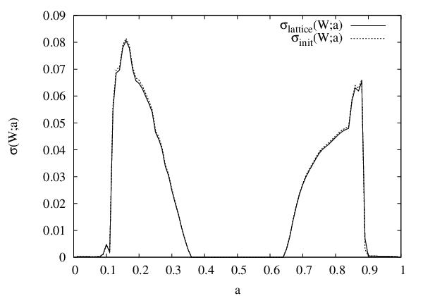
Fig. 1 shows the result of our numerical calculation for the six interesting string dynamics as a function of the coupling $a$. Apparently both $\sigma_{\mathrm{init}}(W;a)$ and $\sigma_{\mathrm{lattice}}(W;a)$ show nearly identical behaviour and are non-vanishing for large ranges of the coupling parameter $a$, thus indicating non-ergodic behaviour.

We may also look at the joined inhomogeneity measure $\sigma(W;a)$ given by

$$\sigma(W;a)=\sqrt{\left<(W^{i,j}(a))^{2}\right>_{\mathrm{lattice},\Phi_{0}}-\left<W^{i,j}(a)\right>^{2}_{\mathrm{lattice},\Phi_{0}}},$$

(55)

where the standard deviation is now simulataneously determined from an average over all initial values and all lattice sites. For a finite number of iterations $T$ and for finite lattice sizes statistical disorder will prevent a completely vanishing standard deviation. As a criterium to distinguish between an inhomogeneous non-ergodic dynamics and a homogeneous ergodic dynamics with a nonzero $\sigma(W;a)$ due to finite-iteration time statistical fluctuations, we determined $\sigma(W;a)$ as a function of the number of iterations. For statistical fluctuations we expect

$$\sigma(W;a|T)\propto T^{-\frac{1}{2}}$$

(56)

(due to the Central Limit Theorem) whereas for an inhomogeneous (non-ergodic) dynamics we expect

$$\sigma(W;a|T)\approx\mbox{constant}$$

(57)

due to very slow decay of correlations and different attractors in the system. This behaviour is verified in Fig. 2 for some important examples of string dynamics and coupling constants.

In [5] the smallest stable zeros of the interaction energy, i.e. values $a^{*}$ with $W_{[N,s,b]}(a^{*})=0$ and $W^{\prime}_{[N,s,b]}(a^{*})<0$, were used to fix standard model coupling constants from first principles. The idea advocated in [5] is that standard model coupling constants are fixed as states of strongest random properties of chaotic strings, distinguished by a vanishing nearest-neighbour correlation. Interesting enough, in [5] six stable zeros were found for which a direct standard model interpretation was possible. These were the smallest stable zeros 0.0008164, 0.007304, 0.001801, 0.01755 of the $3A$ and $3B$ dynamics, which could be associated with electroweak interactions strengths at the lightest fermionic mass scales, and the smallest stable zeros 0.1201 and 0.09537 of the $2A$ and $2B^{-}$ dynamics, which could be associated with strong interaction strengths at the $W$ and Higgs mass scale, respectively. Two additional stable zeros were found, namely the smallest stable zero $0.1758$ of the $2A^{-}$ string and the smallest stable zero $0.3145$ of the $2B$ string, for which the physical interpretation was by far less obvious. In Fig. 2 the quantity $\sigma(W;a|T)$ is displayed for all these zeros. Interesting enough, we see from this figure that the two zeros that could not be interpreted in a straightforward way in terms of standard model interaction strengths apparently correspond to nonergodic states with non-converging behaviour of type (57). These zeros should thus be discarded from the analysis. On the other hand, the other zeros which do have physical meaning in [5] are observed to correspond to ergodic states with well-defined convergence behaviour. Apparently, physically relevant states of the vacuum should be associated with ergodic behaviour.

References

- [1] K. Kaneko, Progr. Theor. Phys. 72, 480 (1984)
- [2] R. Kapral, Phys. Rev. A 31, 3868 (1985)
- [3] K. Kaneko (ed.), Theory and Applications of Coupled Map Lattices, John Wiley and Sons, New York (1993)
- [4] K. Kaneko, I. Tsuda, Complex Systems: Chaos and Beyond, Springer, Heidelberg (2000)
- [5] C. Beck, Spatio-temporal chaos and vacuum fluctuations of quantized fields, World Scientific, Singapore (2002)
- [6] A. Bunimovich, Ya.G. Sinai, Nonlinearity 1, 491 (1988)
- [7] R.E. Amritkar and P.M. Gade, Phys. Rev. Lett. 70, 3408 (1993)
- [8] S. Jalan, R.E. Amritkar, C.-K. Hu, Phys. Rev. E 72, 016211 (2005)
- [9] R. Carretero-Gonzales, D.K. Arrowsmith and F. Vivaldi, Physica D 103, 381 (1997)
- [10] L.A. Bunimovich, Physica D 103, 1 (1997)
- [11] V. Baladi and H.H. Rugh, Comm. Math. Phys. 220, 561 (2001)
- [12] J. Bricmont, A. Kupiainen, Comm. Math. Phys. 178, 703 (1996)
- [13] E. Järvenpää and M. Järvenpää, Comm. Math. Phys. 220, 1 (2001)
- [14]
V. Baladi, Positive Transfer Operators and Decay of Correlations,
World Scientific, Singapore 2000 - [15] H. Daido, Progr. Theor. Phys. Suppl. 79, 75 (1984)
- [16] A. Lemaître and H. Chaté, Europhys. Lett. 39, 377 (1997)
- [17] W. Yang, E-Jiang Ding and M. Ding, Phys. Rev. Lett. 76, 1808 (1996)
- [18] M.C. Mackey and J. Milton, Physica D 80, 1 (1995)
- [19] G. Keller and M. Künzle, Erg. Th. Dyn. Syst. 12, 297 (1992)
- [20] A. Lemaître, H. Chaté and P. Manneville, Europhys. Lett. 39, 377 (1997)
- [21] H. Chaté and J. Losson, Physica D 103, 51 (1997)
- [22] S. Groote and C. Beck, Phys. Rev. E 74, 046216 (2006)
- [23] S. Groote and C. Beck, Dyn. Syst. 22, 219 (2007)
- [24] C. Beck, Physica D 171, 72 (2002)
- [25] C. Beck, Nonlinearity 8, 423 (1995)
- [26] C. Beck, Phys. Lett. A 248, 386 (1998)
- [27] C. Beck, Phys. Rev. D 69, 123515 (2004)
- [28] C. Beck, hep-th/0702082
- [29] M. Szydlowski, A. Krawiec, W. Czaja, Phys. Rev. E 72, 036221 (2005)
- [30] T.S. Biro, B. Mueller, S.G. Matinyan, hep-lat/0305023
- [31] M. Maher and C. Beck, arXiv: 0801.4720 [hep-th], to appear in Chaos Sol. Fractals (2008)
- [32] C.L. Gardner, Phys. Rev. D 68, 043513 (2003)
- [33]
C. Beck, F. Schlögl, Thermodynamics of Chaotic Systems,
Cambridge University Press, Cambridge 1993 - [34] C. Beck, Nonlinearity 4, 1131 (1991)
- [35] A. Hilgers and C. Beck, Physica D 156, 1 (2001)
- [36] C.P. Dettmann, Physica D 172, 88 (2002)
- [37] C.P. Dettmann and D. Lippolis, Chaos Sol. Fractals 23, 43 (2005)