Transverse NMR relaxation in magnetically heterogeneous media

A spin traveling along Brownian path ${\bf r}(t)$ originating at ${\bf r}(0)={\bf r}_{0}$, acquires the relative phase $\exp\left\{-i\int_{0}^{t}\!dt\,\Omega[{\bf r}(t)]\right\}$. Here $\Omega({\bf r})$ is the variable component of the Larmor frequency; $\left<\Omega({\bf r})\right>\equiv 0$. The time evolution

of the magnetization packet initially at ${\bf r}={\bf r}_{0}$, ${\cal G}({\bf r}_{0},{\bf r},t)|_{t=0}=\delta({\bf r}-{\bf r}_{0})$, is the precession phase averaged over the Wiener measure on the diffusive paths. Equivalently, ${\cal G}({\bf r}_{0},{\bf r};t)$ is the Green’s function (fundamental solution) of the Bloch-Torrey equation [28]

The diffusive dynamics (3) leads to the transverse relaxation, ${\cal G}({\bf r}_{0},{\bf r},t)|_{t\to\infty}=0$.

For simplicity, and in order to underscore the effects of susceptibility contrast, below we assume homogeneous diffusivity $D({\bf r})\equiv D={\rm const}$. We also excluded conventional exponential factors associated with homogeneous components of Larmor frequency and of transverse relaxation.

The mesoscopic component $s(t)$ of the measured MR signal (normalized to $s|_{t=0}\equiv 1$) is obtained in two stages. First, one considers the signal $s_{\Omega}$ from a given realization of $\Omega({\bf r})$. It is given by the magnetization ${\cal G}({\bf r}_{0},{\bf r};t)$ that is summed over the final positions ${\bf r}$ which spins reach during the time interval $t$, and averaged over initial spin positions ${\bf r}_{0}$. The signal $s(t)$ is then found by averaging of $s_{\Omega}$ over all realizations of $\Omega({\bf r})$,

Here we used the translation invariance of the distribution-averaged Green’s function $\left<{\cal G}({\bf r}_{0},{\bf r};t)\right>\equiv G({\bf r}-{\bf r}_{0},t)$, with its Fourier components defined as $G_{\omega,{\bf k}}=\int\!dtd{\bf r}\,G({\bf r},t)e^{i\omega t-i{\bf k}{\bf r}}$.

Eq. (4) connects the spectral lineshape $s(\omega)=G_{\omega,{\bf k}}|_{{\bf k}=0}$ with the distribution-averaged Green’s function of Eq. (3). The result of such an averaging (see Methods) may be represented as

where the diffusion propagator

is the Green’s function of Eq. (3) with $\Omega\equiv 0$.

The generic representation (5) yields the dynamics $\omega=\omega({\bf k})$ as the pole of the propagator $G_{\omega,{\bf k}}$, modified by interaction with complex environment embodied in $\Sigma_{\omega,{\bf k}}$ [25]. For the ballistic dynamics, expansion of $\Sigma_{\omega,{\bf k}}$ would give the refraction index of the medium (when $\omega\propto k$), or the renormalized quasiparticle mass and lifetime (when $\omega\propto k^{2}$). In the present case of the diffusive dynamics (3) ($i\omega\propto k^{2}$), the self-energy $\Sigma_{\omega,{\bf k}}$ contains all the measurable information about mesoscopic relaxation. In particular, its expansion $\Sigma_{\omega,{\bf k}}=\Sigma(0)-(\delta D)k^{2}+...$ in $\omega$ and ${\bf k}$ describes the effect of the mesoscopic relaxation on the coarse-grained dynamics of the magnetization density. In other words, Eq. (5), viewed as an operator relation, is the effective Bloch-Torrey equation, that acquires higher derivatives in $t$ and ${\bf r}$, after averaging over the medium. According to Eq. (4), the signal lineshape (1) is a particular case of (5) with

As a simplest example we now consider the weakly magnetic medium whose Larmor frequency dispersion $\delta\Omega\equiv\sqrt{\left<\Omega^{2}\right>}$ is small, and find the relaxation in the lowest order in $(\delta\Omega)^{2}\equiv\Gamma_{2}({\bf r})|_{{\bf r}=0}$. The self-energy is given by the single Feynman graph (see Methods, Fig. 4(c)),

The lowest order contribution to the self-energy part for the signal,

involves only the angular-averaged two-point correlation function $\overline{\Gamma_{2}}(q)=\left<\Gamma_{2}({\bf q})\right>_{\hat{\bf q}}$. Eq. (9) is the Gaussian approximation in a weakly paramagnetic medium. Corrections to this approximation, involving correlators $\Gamma_{n}$, first appear in the $n$-th order in the Born series for $\Sigma_{\omega,{\bf k}}$.

Equation (9) gives the universal short-time asymptotic behavior: In the limit $\omega\to\infty$ this is the leading in $1/\omega$ contribution to $\Sigma(\omega)$, yielding $\Sigma(\omega)|_{\omega\to\infty}\simeq(\delta\Omega)^{2}/i\omega$. Substituting it into Eq. (1) and taking the inverse Fourier transform, results in $s(t)|_{t\to 0}\simeq 1-(\delta\Omega\cdot t)^{2}/2$, for $\delta\Omega\cdot t\ll 1$.

The diffusing spins sense the distribution of the Larmor frequency offset $\Omega({\bf r})$. Often times, in paramagnetic media, such a distribution is induced by a variable magnetic susceptibility profile $\chi({\bf r})$, which is practically interesting. Then the medium is characterized by the correlation functions of $\chi$, assuming zero average $\left<\chi\right>=0$. In particular, here we consider the two-point correlation function $\Gamma_{2}^{\chi}(r)=\left<\chi({\bf r})\chi(0)\right>$ that for a statistically isotropic medium depends only on $r=|{\bf r}|$. For nonferromagnetic media, such as deoxygenated blood, $|\chi|\ll 1$, hence the induced field $\Omega({\bf r})$ is connected to $\chi({\bf r})$ by the convolution with an elementary dipole field $Y({\bf r})$,

Here $\Omega_{0}$ is the uniform Larmor frequency component, and $Y({\bf r})$ includes both the local contribution $\propto\delta({\bf r})$, and the Lorentz cavity field, that compensate each other in three dimensions [29, 30].

The angular-averaged correlators of Larmor frequency and of the underlying susceptibility are proportional to each other (locality [22]):

Here $Y(\hat{\bf k})$ is the Fourier transform of the dipole field; in $d=3$ dimensions, $Y(\hat{\bf k})=1/3-{k_{z}^{2}/k^{2}}$, and Eq. (12) yields $\lambda^{2}=4/{45}$. In $d=2$ dimensions, $Y(\hat{\bf k})=1/2-{k_{y}^{2}/k^{2}}$, yielding $\lambda^{2}=1/8$.

To prove Eq. (11), we note that the Fourier transform of the field $\Omega$ induced by the susceptibility profile with the orientation ${\cal R}$ is $\Omega_{\cal R}({\bf k})=4\pi\Omega_{0}Y(\hat{\bf k})\chi({\cal R}^{-1}{\bf k})$. Substituting $\Omega_{\cal R}$ into first Eq. (11) and averaging over orientations ${\cal R}$ yields the right-hand side. Physically, we went from averaging over the orientations ${\cal R}$ of the medium relative to a given $\hat{\bf z}$-direction of the main field $B_{0}\hat{\bf z}$ to averaging over the direction of the field at fixed orientation of the structure $\chi({\bf r})$.

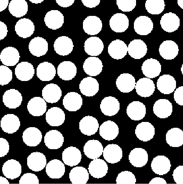
The locality property (11) means that, in the second order in $\Omega$, after the orientational averaging the diffusing spins effectively interact directly with the susceptibility profile $\chi({\bf r})$, via $4\pi\lambda\Omega_{0}\chi({\bf r})$. This interaction is much simpler than that with the susceptibility-induced field $\Omega({\bf r})$, which involves a convolution with the non-local field (10) with a complicated angular dependence. The underlying reason for this fortunate property is the scaling $Y({\bf r})\propto r^{-d}$ in $d$ dimensions [22]. The locality (11) is demonstrated for the two-dimensional numerically generated medium in Fig. 1.

Aimed at relating the signal to the magnetic structure, we consider the medium, embodied by the distribution of $\chi({\bf r})$, that has a single mesoscopic length scale $l_{c}$. This scale, and the dispersion $\delta\Omega$, are the two parameters that we employ here to characterize the medium.

For the model calculations below we focus on the angular-averaged correlation function $\overline{\Gamma_{2}}$ entering Eq. (9). The presence of a single length scale leads to a well-defined dominant peak in the function $\overline{\Gamma_{2}}(k)$. Such a form is demonstrated for the $d=2$ case in Fig. 1(c). We suggest to approximate such a peak via a delta-function

normalized to $\int\!{d^{d}{\bf k}\over(2\pi)^{d}}\,\overline{\Gamma_{2}}\equiv(\delta\Omega)^{2}$, assuming that the contribution of other length scales is less relevant. In real space, the correlator (13)

In $d=2$ dimensions, the corresponding correlator is $\overline{\Gamma_{2}}(k)=(\delta\Omega)^{2}l_{c}\delta(k-k_{c})$ and $\overline{\Gamma_{2}}(r)=(\delta\Omega)^{2}J_{0}(k_{c}r)$, where $J_{0}$ is the Bessel function. Generalization onto the case when the medium has a set of harmonics (14) with different $k_{c}$ is straightforward: e.g. for $d=3$,

With the approximation (13), evaluation of self-energy (9) in the lowest order is trivial:

Here we introduced the diffusion time

past the Larmor frequency correlation length $l_{c}=2\pi/k_{c}$. Time $t_{c}$ sets the scale for both the frequency $\omega$ and for the self-energy. The dimensionless perturbation series parameter

controls the dephasing strength.

The lineshape (1), (16) is a sum of the two Lorentzians

where (keeping terms up to the order $\alpha^{2}$)

and the weights $w_{1}=-\alpha^{2}$ and $w_{2}=1+\alpha^{2}$. The approach (9) is valid for $\alpha\ll 1$. The signal $s(t)\simeq 1-\textstyle{\frac{1}{2}}\alpha^{2}(t/t_{c})^{2}$ for $t\ll t_{c}$, and decays monoexponentially for $t\to\infty$ as $s\simeq w_{2}\exp\{-t/T_{2}^{\rm pert}\}$ with the rate $1/T_{2}^{\rm pert}=\alpha^{2}/t_{c}=(\delta\Omega)^{2}t_{c}$. The latter rate arises due to angular diffusion of the precession phase: As the phase changes by $\sim\alpha$ at each time step $t_{c}$, over large time $t\gg t_{c}$ the rms phase $\sim\alpha\sqrt{t/t_{c}}$ reaches $\sim 1$ for $t\sim T_{2}^{\rm pert}$ (Dyakonov-Perel relaxation [31]). The relaxation rate decreases with decreasing $l_{c}$, as the medium effectively becomes more homogeneous (diffusion narrowing).

What happens in a complex medium with a few harmonics, Eq. (15)? In the lowest order, ${\cal O}\left((\delta\Omega)^{2}\right)$, harmonics with different ${l_{c}}_{j}$ and dephasing strengths $\alpha_{j}=\sqrt{p_{j}}\,\delta\Omega\cdot{t_{c}}_{j}$ contribute to the self-energy (9) additively. Thus $\Sigma(\omega)$ is a sum of $n$ terms (16), and the lineshape is a sum of $n+1$ Lorentzians that correspond to the presence of $n$ distinct length scales.

We emphasize that the apparent $n+1$-exponential form of the perturbative result $s(t)$ (biexponential (20) for $n=1$) here has nothing to do with existence of $n+1$ macroscopic “compartments” with different relaxation rates. (Note also that the weight $w_{1}<0$ in Eq. (20).) This simple example is a warning against common practice of literally interpreting bi- or multi-exponential fits.

The $t\to\infty$ relaxation is determined by the pole of signal (1) closest to real axis. For weak dephasing, such a pole is given by $i\Sigma^{\rm pert}(0)$, yielding additive contributions for the total rate $1/T_{2}^{\rm pert}=\sum_{j=1}^{n}\alpha_{j}^{2}/{t_{c}}_{j}$ similar to the Matthiessen rule in kinetic theory. Equivalently,

(This result can be already deduced from Eq. (9) by setting there $\omega=0$.)

The rate (22) is formally equivalent to the Coulomb energy of a fictitious charge distribution with the charge density $\Omega({\bf r})$ [or of $4\pi\lambda\Omega_{0}\chi({\bf r})$ via locality]. Extending this mapping, the variable diffusivity $D({\bf r})$ would be analogous to a variable dielectric constant. Equivalence of (22) with Coulomb problem is due to the Laplace form of Eq. (3). In the limit $t\to\infty$, relaxation is determined by the diffusing spins wandering infinitely far to explore the magnetic structure. The spins then become mediators of the effectively long-ranged interaction between the different parts of the magnetic structure. The long-time asymptote corresponds to the time-averaged diffusion propagator which becomes a Coulomb potential, $\int_{0}^{\infty}\!dt\,{G^{0}}({\bf r},t)\propto 1/r$.

The self-energy (9), as well as the rate (22), strongly depend on the geometric structure, as the convergence of integrals is determined by the specific way of how $\Gamma_{2}$ vanishes at short distances (large $k$). This nonuniversality can be also seen from mapping onto Coulomb problem, since $T_{2}^{\rm pert}$ maps onto capacitance which is sensitive to the conductor geometry.

The self-energy (9) substituted into the lineshape (1) is a natural extension of the results [22] (rederived in a different way in [23, 24]) to the case of arbitrary volume fraction $\zeta$. The signal takes the form $s(t)=\exp[-f(t)]$, where

Indeed, while $f(t)\ll 1$, Eq. (23) is the lowest order expansion of (1) in $\Sigma$, valid for $t\ll t_{c}/\alpha^{2}$. For $t\gg t_{c}$, Eq. (23) yields the same relaxation rate as Eqs. (1) and (9). As these two time domains overlap, the equivalence is proven for all $t$. Relaxation in the dilute suspension is just a particular case of (23), with $\Gamma_{2}\simeq\zeta\Gamma_{2}^{(1)}$, where $\Gamma_{2}^{(1)}$ is the correlator for a single object.

Below we attempt to go beyond the perturbative calculation and explore the case of moderate dephasing, $\alpha\lesssim 1$. An exact solution would amount to summing up all the diagrams for the self-energy to all orders in $\alpha$, an arduous task even within a simplifying assumption (13). Here we consider the self-energy in the self-consistent Born approximation (SCBA)

Technically, Eq. (24) amounts to summing all the non-crossing Feynman graphs (see Methods, Fig. 4). The SCBA is akin to mean field theory (more precisely, it is equivalent to the mean field treatment of the nonlinear term that arises after Gaussian disorder-averaging in the replica field theory). Its advantage is that one can move quite far analytically, by summing up an infinite subset of Feynman graphs, thereby collecting contributions from all orders in the external random field $\Omega({\bf r})$. Its disadvantage is that it is uncontrolled since it leaves out an infinite subset of graphs for $\Sigma_{\omega,{\bf k}}$.

Eq. (24) is a complicated integral equation for $\Sigma_{\omega,{\bf k}}$ due to the ${\bf k}$-dependence of $\Sigma$ on the right-hand side. Since we really only need $\Sigma|_{k=0}$, we now make another (uncontrolled) simplification that will lead to an ansatz for $\Sigma(\omega)$. Neglecting the $k$-dependence of the self-energy in the denominator, we obtain the quadratic equation

whose solution is

The sign in front of the square root $R(\omega)$ in Eq. (26) agrees with the perturbative solution (16).

To summarize, both the lowest order signal (19) and the SCBA are perturbative expressions. However, the lowest order approximation (19) is valid for $\alpha\ll 1$, while utilizng the SCBA allows us to work up until $\alpha\lesssim 1$ (as described below). This “convergence enhancement”, while questionable mathematically, appears to be quite useful practically, as we demonstrate below both by comparing the self-energy (26) to the Monte Carlo simulations, and by applying it to interpret proton spectra in human blood.

In Fig. 2 we compare the above results with Monte Carlo simulation of diffusion and relaxation in the 2d medium described in Fig. 1. The numerical self-energy was calculated according to Eq. (1) after adjusting central frequency of $s(\omega)$ for a small shift $\left<\Omega\right>$ due to higher-order correlators.

Practically, the perturbative self-energy (9) agrees perfectly with numerics for $\alpha\lesssim 0.3$. For these values of $\alpha$ the characteristic “triangular” shape of $\mbox{\,Re\,}\Sigma(\omega)$ deviates from simple Lorentzian (16) due to contribution of harmonics with $k<k_{c}$. Interestingly, for intermediate $\alpha\sim 0.5$, the shape of $\Sigma(\omega)$ becomes qualitatively closer to the Lorentzian (16). Indeed, for larger $\alpha$, spins dephase before they can explore the scales exceeding $l_{c}$, which increases the relative contribution of large-$k$ harmonics.

Quantitatively, the SCBA ansatz (26) is notably better than both (9) and (16) for $\alpha\gtrsim 0.5$. One can attain a perfect agreement of SCBA with the data by allowing $\alpha$ and $t_{c}$ to be fitting parameters; at $\alpha\gtrsim 1$, the SCBA fit values gradually deviate from the geniune parameters, as illustrated in Fig. 2(d). This is a consequence of the properties of the SCBA signal (1), (26) in the complex plane of $z=\omega t_{c}$: When $\alpha>1$, the simple pole of (1) at $z=-i\alpha^{2}$ dives under the branch cut connecting $z=-i\pm 2\alpha$. Physically, the developed perturbative approach must break down for $\alpha\gtrsim 1$, as the system crosses over from the diffusion-narrowing to static dephasing regime, $\alpha\gg 1$. The signal in the latter limit coincides with the characteristic function of the probability distribution of the local Larmor frequency, $s(t)=\left<e^{-i\Omega({\bf r})t}\right>$. The connection of $s(\omega)$ to the mesoscopic structure in this limit was studied only for dilute suspensions of objects with basic geometries [32, 33, 34, 35, 36, 20, 21].

We now apply our general results to interpret the line shape of water protons in blood as measured by Bjørnerud et al. [27]. Blood plasma was titrated with a superparamagnetic contrast agent to match the magnetic susceptibility of deoxygenated red blood cells. The mesoscopic magnetic structure originated from the susceptibility contrast between plasma and oxygenated haemoglobin in erythrocytes.

Our model and the expression (26) for the lineshape has been obtained assuming unrestricted diffusion (uniform diffusivity $D$). Strictly speaking, the assumption of homogeneous diffusivity does not hold for blood. Below we partially account for the hindered diffusion in blood by using the reduced apparent diffusion coefficient (ADC) of blood [37]. This is a reasonable approximation in view of the fast exchange through the cell membrane [38, 39].

We have calculated the corresponding self-energy from the data of Ref. [27] in three stages: First, the imaginary part $\mbox{\,Im\,}s(\omega)$ was determined using the Kramers-Krönig relations from the published $\mbox{\,Re\,}s(\omega)$. Special attention was paid to phase correction procedure that allowed to cancel the residual uniform Larmor frequency offset. Second, the self-energies $\Sigma_{\rm oxy}$ and $\Sigma_{\rm deoxy}$ for the oxygenated and deoxygenated states respectively were determined according to Eq. (1). Finally, the difference $\Sigma(\omega)=\Sigma_{\rm oxy}-\Sigma_{\rm deoxy}$ was formed in order to cancel microscopic effects and reduce data processing errors.

As demonstrated in Fig. 3, the functional shape (26) agrees very well with the self-energy $\Sigma(\omega)$. The parameters from fitting $\mbox{\,Re\,}\Sigma(\omega)$ are $\alpha^{\rm fit}=1.3$, $t_{c}^{\rm fit}=1.5\,$ms, yielding $\delta\Omega^{\rm fit}\approx 0.86$ ms^-1, and $l_{c}\approx 2.9\,\mu$m assuming the blood ADC value $D=1.1\,\mu{\rm m}^{2}$/ms at the temperature $T=37\,$C of the measurement [27] (we calculated this ADC value from the mean diffusivity of the blood ADC measured at 25 C [37] asuming Arrhenius temeprature dependence similar to that of water). Fitting of Im $\Sigma$ gives results within 5%. The value $\delta\Omega^{\rm fit}$ is in a reasonable agreement with the experimental $\delta\Omega=0.69$ ms^-1. The value of $l_{c}$ matches the size of the doughnut-shaped erythrocytes with large diameter $7\,\mu$m and thickness about $2\,\mu$m.

References

- [1] J. A. Glasel, K. H. Lee, On the interpretation of water nuclear magnetic resonance relaxation times in heterogeneous systems, J Amer. Chem. Soc. 96 (1974) 970 – 978.
- [2] D. D. Awschalom, D. Loss, N. Samarth (Eds.), Semiconductor Spintronics and Quantum Information, Springer, New York, 2002.
- [3] M. M.T. Vlaardingerbroek, J. den Boer, Magnetic Resonance Imaging. Theory and Practice, 2nd Edition, Springer, New York, 1999.
- [4] G. Eaton, S. S. Eaton, K. Ohno (Eds.), EPR Imaging and in Vivo EPR, CRC Press, Boston, 1991.
- [5] S. A. Crooker, D. D. Awschalom, J. J. Baumberg, F. Flack, N. Samarth, Optical spin resonance and transverse spin relaxation in magnetic semiconductor quantum wells,, Phys Rev B 56 (1997) 7574–7588.
- [6] J. M. Kikkawa, I. P. Smorchkova, N. Samarth, D. D. Awschalom, Room temperature spin memory in two-dimensional electron gases, Science 277 (1997) 1284–1287.
- [7] J. M. Kikkawa, D. D. Awschalom, Resonant spin amplification in -type GaAs, Phys Rev Lett 80 (1998) 4313–4316.
- [8] G. Salis, Y. Kato, K. Ensslin, D. Driscoll, A. Gossard, D. Awschalom, Electrical control of spin coherence in semiconductor nanostructures, Nature 414 (2001) 619–622.
- [9] W. H. Lau, V. Sih, N. P. Stern, R. C. Myers, D. A. Buell, A. C. Gossard, D. D. Awschalom, Room temperature electron spin coherence in telecom-wavelength quaternary quantum wells, Appl Phys Lett 89 (2006) 142104.
- [10] S. Ogawa, T. Lee, A. Nayak, P. Glynn, Oxygenation-sensitive contrast in magnetic resonance image of rodent brain at high magnetic fields, Magn Reson Med 14 (1990) 68–78.
- [11] S. Ogawa, T. Lee, Magnetic resonance imaging of blood vessels at high fields: in vivo and in vitro measurements and image simulation, Magn Reson Med 16 (1990) 9–18.
- [12] J. Belliveau, D. Kennedy, R. McKinstry, B. Buchbinder, R. Weisskoff, M. Cohen, J. Vevea, T. Brady, B. Rosen, Functional mapping of the human visual cortex by magnetic resonance imaging., Science 254 (5032) (1991) 716–9.
- [13] K. Kwong, J. Belliveau, D. Chesler, I. Goldberg, R. Weisskoff, B. Poncelet, D. Kennedy, B. Hoppel, M. Cohen, R. Turner, Dynamic magnetic resonance imaging of human brain activity during primary sensory stimulation., Proc Natl Acad Sci U S A 89 (12) (1992) 5675–9.
- [14] P. A. Bandettini, E. C. Wong, R. S. Hinks, R. S. Tikofsky, J. S. Hyde, Time course EPI of human brain function during task activation, Magn Reson Med 25 (2) (1992) 390–397.
- [15] R. S. Menon, S. Ogawa, S. G. Kim, J. M. Ellermann, H. Merkle, D. W. Tank, K. Ugurbil, Functional brain mapping using magnetic resonance imaging. signal changes accompanying visual stimulation, Invest Radiol 27 Suppl 2 (1992) 47–53.
- [16] P. Gillis, S. Koenig, Transverse relaxation of solvent protons induced by magnetized spheres: application to ferritin, erythrocytes, and magnetite., Magn Reson Med 5 (4) (1987) 323–345.
- [17] R. P. Kennan, J. Zhong, J. C. Gore, Intravascular susceptibility contrast mechanisms in tissues., Magn Reson Med 31 (1) (1994) 9–21.
- [18] V. G. Kiselev, S. Posse, Analytical theory of susceptibility induced NMR signal Dephasing in a Cerebrovascular Network, Physical Review Letters 81 (1998) 5696 – 5699.
- [19] J. Jensen, R. Chandra, NMR relaxation in tissues with weak magnetic inhomogeneities., Magn Reson Med 44 (1) (2000) 144–56.
- [20] W. R. Bauer, W. Nadler, M. Bock, L. R. Schad, C. Wacker, A. Hartlep, G. Ertl, Theory of coherent and incoherent nuclear spin dephasing in the heart, Phys. Rev. Lett. 83 (1999) 4215 – 4218.
- [21] W. R. Bauer, W. Nadler, Spin dephasing in the extended strong collision approximation., Phys Rev E Stat Nonlin Soft Matter Phys 65 (6 Pt 2) (2002) 066123.
- [22] V. G. Kiselev, D. S. Novikov, Transverse NMR relaxation as a probe of mesoscopic structure, Physical Review Letters 89 (2002) 278101.
- [23] A. L. Sukstanskii, D. A. Yablonskiy, Gaussian approximation in the theory of MR signal formation in the presence of structure-specific magnetic field inhomogeneities., J Magn Reson 163 (2) (2003) 236–247.
- [24] A. L. Sukstanskii, D. A. Yablonskiy, Gaussian approximation in the theory of MR signal formation in the presence of structure-specific magnetic field inhomogeneities. Effects of impermeable susceptibility inclusions., J Magn Reson 167 (1) (2004) 56–67.
- [25] A. Abrikosov, L. Gorkov, I. Dzyaloshinski, Methods of Quantum Field Theory in Statistical Physics, Prentice-Hall, Englewood Cliffs, 1963.
- [26] P. W. Kuchel, B. T. Bulliman, Perturbation of homogeneous magnetic fields by isolated single and confocal spheroids. implications for nmr spectroscopy of cells., NMR Biomed 2 (4) (1989) 151–160.
- [27] A. Bjørnerud, K. Briley-Saebø, L. O. Johansson, K. E. Kellar, Effect of NC100150 injection on the (1)H NMR linewidth of human whole blood ex vivo: dependency on blood oxygen tension., Magn Reson Med 44 (5) (2000) 803–807.
- [28] H. C. Torrey, Bloch equations with diffusion terms, Phys. Rev. 104 (1956) 563.
- [29] J. Jackson, Classical Electrodynamics, 2nd Edition, Wiley, New York, 1975.
- [30] W. Dickinson, The time average magnetic field at the nucleus in nuclear magnetic resonance experiments, Physical Review 81 (1951) 717–731.
- [31] M. Dyakonov, V. Perel, Spin orientation of electrons associated with interband absorption of light in semiconductors,, Sov Phys JETP 33 (1971) 1053.
- [32] D. A. Yablonskiy, E. M. Haacke, Theory of NMR signal behavior in magnetically inhomogeneous tissues: the static dephasing regime., Magn Reson Med 32 (6) (1994) 749–763.
- [33] V. G. Kiselev, S. Posse, Analytical model of susceptibility-induced MR signal dephasing: Effect of diffusion in a microvascular network, Magn Reson Med 41 (1999) 499–509.
- [34] J. Jensen, R. Chandra, Strong field behavior of the NMR signal from magnetically heterogeneous tissues., Magn Reson Med 43 (2) (2000) 226–36.
- [35] V. G. Kiselev, On the theoretical basis of perfusion measurements by dynamic susceptibility contrast MRI, Magn Reson Med 46 (2001) 1113 – 1122.
- [36] A. Sukstanskii, D. Yablonskiy, Theory of FID NMR signal dephasing induced by mesoscopic magnetic field inhomogeneities in biological systems., J Magn Reson 151 (1) (2001) 107–17.
- [37] P. W. Kuchel, C. J. Durrant, B. E. Chapman, P. S. Jarrett, D. G. Regan, Evidence of red cell alignment in the magnetic field of an nmr spectrometer based on the diffusion tensor of water., J Magn Reson 145 (2) (2000) 291–301.
- [38] G. Benga, V. I. Pop, O. Popescu, A. Hodârnău, V. Borza, E. Presecan, Effects of temperature on water diffusion in human erythrocytes and ghosts–nuclear magnetic resonance studies., Biochim Biophys Acta 905 (2) (1987) 339–348.
- [39] A. R. Waldeck, M. H. Nouri-Sorkhabi, D. R. Sullivan, P. W. Kuchel, Effects of cholesterol on transmembrane water diffusion in human erythrocytes measured using pulsed field gradient nmr., Biophys Chem 55 (3) (1995) 197–208.
- [40] L. Landau, E. Lifshitz, Quantum Mechanics: Non-Relativistic Theory, Butterworth–Heinemann, Oxford, 1981.