On the Distribution of the Adaptive LASSO Estimator

Benedikt M. Pötscher Ulrike Schneider Affiliation: Department of Statistics, University of Vienna

First version: December 2007
This version: December 2008

Abstract

We study the distribution of the adaptive LASSO estimator (Zou (2006)) in finite samples as well as in the large-sample limit. The large-sample distributions are derived both for the case where the adaptive LASSO estimator is tuned to perform conservative model selection as well as for the case where the tuning results in consistent model selection. We show that the finite-sample as well as the large-sample distributions are typically highly non-normal, regardless of the choice of the tuning parameter. The uniform convergence rate is also obtained, and is shown to be slower than $n^{-1/2}$ in case the estimator is tuned to perform consistent model selection. In particular, these results question the statistical relevance of the ‘oracle’ property of the adaptive LASSO estimator established in Zou (2006). Moreover, we also provide an impossibility result regarding the estimation of the distribution function of the adaptive LASSO estimator. The theoretical results, which are obtained for a regression model with orthogonal design, are complemented by a Monte Carlo study using non-orthogonal regressors.

MSC 2000 subject classification. Primary 62F11, 62F12, 62E15, 62J05, 62J07.

Key words and phrases. Penalized maximum likelihood, LASSO, adaptive LASSO, nonnegative garotte, finite-sample distribution, asymptotic distribution, oracle property, estimation of distribution, uniform consistency.

1 Introduction

Penalized maximum likelihood estimators have been studied intensively in the last few years. A prominent example is the least absolute selection and shrinkage (LASSO) estimator of Tibshirani (1996). Related variants of the LASSO include the Bridge estimators studied by Frank & Friedman (1993), least angle regression (LARS) of Efron et al. (2004), or the smoothly clipped absolute deviation (SCAD) estimator of Fan & Li (2001). Other estimators that fit into this framework are hard- and soft-thresholding estimators. While many properties of penalized maximum likelihood estimators are now well understood, the understanding of their distributional properties, such as finite-sample and large-sample limit distributions, is still incomplete. The probably most important contribution in this respect is Knight & Fu (2000) who study the asymptotic distribution of the LASSO estimator (and of Bridge estimators more generally) when the tuning parameter governing the influence of the penalty term is chosen in such a way that the LASSO acts as a conservative model selection procedure (that is, a procedure that does not select underparameterized models asymptotically, but selects overparameterized models with positive probability asymptotically). In Knight & Fu (2000), the asymptotic distribution is obtained in a fixed-parameter as well as in a standard local alternatives setup. This is complemented by a result in Zou (2006) who considers the fixed-parameter asymptotic distribution of the LASSO when tuned to act as a consistent model selection procedure. Another contribution is Fan & Li (2001) who derive the fixed-parameter asymptotic distribution of the SCAD estimator when the tuning parameter is chosen in such a way that the SCAD estimator performs consistent model selection; in particular, they establish the so-called ‘oracle’ property for this estimator. Zou (2006) introduced a variant of the LASSO, the so-called adaptive LASSO estimator, and established the ‘oracle’ property for this estimator when suitably tuned. Since it is well-known that fixed-parameter (i.e., pointwise) asymptotic results can give a wrong picture of the estimator’s actual behavior, especially when the estimator performs model selection (see, e.g., Kabaila (1995), or Leeb & Pötscher (2005), Pötscher & Leeb (2007), Leeb & Pötscher (2008b)), it is important to take a closer look at the actual distributional properties of the adaptive LASSO estimator.

In the present paper we study the finite-sample as well as the large-sample distribution of the adaptive LASSO estimator in a linear regression model. In particular, we study both the case where the estimator is tuned to perform conservative model selection as well as the case where it is tuned to perform consistent model selection. We find that the finite-sample distributions are highly non-normal (e.g., are often multimodal) and that a standard fixed-parameter asymptotic analysis gives a highly misleading impression of the finite-sample behavior. In particular, the ‘oracle’ property, which is based on a fixed-parameter asymptotic analysis, is shown not to provide a reliable assessment of the estimators’ actual performance. For these reasons, we also obtain the large-sample distributions of the above mentioned estimators under a general “moving parameter” asymptotic framework, which much better captures the actual behavior of the estimator. [Interestingly, it turns out that in case the estimator is tuned to perform consistent model selection a “moving parameter” asymptotic framework more general than the usual $n^{-1/2}$ -local asymptotic framework is necessary to exhibit the full range of possible limiting distributions.] Furthermore, we obtain the uniform convergence rate of the adaptive LASSO estimator and show that it is slower than $n^{-1/2}$ in the case where the estimator is tuned to perform consistent model selection. This again exposes the misleading character of the ‘oracle’ property. We also show that the finite-sample distribution of the adaptive LASSO estimator cannot be estimated in any reasonable sense, complementing results of this sort in the literature such as Leeb & Pötscher (2006a), Leeb & Pötscher (2006b), Pötscher & Leeb (2007), Leeb & Pötscher (2008a) and Pötscher (2006).

Apart from the papers already mentioned, there has been a recent surge of publications establishing the ‘oracle’ property for a variety of penalized maximum likelihood or related estimators (e.g., Bunea (2004), Bunea & McKeague (2005), Fan & Li (2002), Fan & Li (2004), Li & Liang (2007), Wang & Leng (2007), 26, 27, 28, Yuan & Lin (2007), Zhang & Lu (2007), Zou & Yuan (2008), Zou & Li (2008), Johnson et al. (2008)). The ‘oracle’ property also paints a misleading picture of the behavior of the estimators considered in these papers; see the discussion in Leeb & Pötscher (2005), Yang (2005), Pötscher (2007), Pötscher & Leeb (2007), Leeb & Pötscher (2008b).

The paper is organized as follows. The model and the adaptive LASSO estimator are introduced in Section 2. In Section 3 we study the estimator theoretically in an orthogonal linear regression model. In particular, the model selection probabilities implied by the adaptive LASSO estimator are discussed in Section 3.1. Consistency, uniform consistency, and uniform convergence rates of the estimator are the subject of Section 3.2. The finite-sample distributions are derived in Section 3.3.1, whereas the asymptotic distributions are studied in Section 3.3.2. We provide an impossibility result regarding the estimation of the adaptive LASSO’s distribution function in Section 3.4. Section 4 studies the behavior of the adaptive LASSO estimator by Monte Carlo without imposing the simplifying assumption of orthogonal regressors. We finally summarize our findings in Section 5. Proofs and some technical details are deferred to an appendix.

2 The Adaptive LASSO Estimator

We consider the linear regression model

Y=X\theta+u

(1)

where $X$ is a nonstochastic $n\times k$ matrix of rank $k$ and $u$ is multivariate normal with mean zero and variance-covariance matrix $\sigma^{2}I_{n}$ . Let $\hat{\theta}_{LS}=(X^{\prime}X)^{-1}X^{\prime}Y$ denote the least squares (maximum likelihood) estimator. The adaptive LASSO estimator $\hat{\theta}_{A}$ is defined as the solution to the minimization problem

(Y-X\theta)^{\prime}(Y-X\theta)+2n\mu_{n}^{2}\sum_{i=1}^{k}|\theta_{i}|/|\hat{\theta}_{LS,i}|

(2)

where the tuning parameter $\mu_{n}$ is a positive real number. As long as $\hat{\theta}_{LS,i}\neq 0$ for every $i$ , the function given by (2) is well-defined and strictly convex and hence has a uniquely defined minimizer $\hat{\theta}_{A}$ . [The event where $\hat{\theta}_{LS,i}=0$ for some $i$ has probability zero under the probability measure governing $u$ . Hence, it is inconsequential how we define $\hat{\theta}_{A}$ on this event; for reasons of convenience, we shall adopt the convention that $\mu_{n}^{2}/|\hat{\theta}_{LS,i}|=0$ if $\hat{\theta}_{LS,i}=0$ . Furthermore, $\hat{\theta}_{A}$ is a measurable function of $Y$ .] Note that Zou (2006) uses $\lambda_{n}=2n\mu_{n}^{2}$ as the tuning parameter. Zou (2006) also considers versions of the adaptive LASSO estimator for which $|\hat{\theta}_{LS,i}|$ in (2) is replaced by $|\hat{\theta}_{LS,i}|^{\gamma}$ . However, we shall exclusively concentrate on the leading case $\gamma=1$ . As pointed out in Zou (2006), the adaptive LASSO is closely related to the nonnegative Garotte estimator of Breiman (1995).

3 Theoretical Analysis

For the theoretical analysis in this section we shall make some simplifying assumptions. First, we assume that $\sigma^{2}$ is known, whence we may assume without loss of generality that $\sigma^{2}=1$ . Second, we assume orthogonal regressors, i.e., $X^{\prime}X$ is diagonal. The latter assumption will be removed in the Monte Carlo study in Section 4. Orthogonal regressors occur in many important settings, including wavelet regression or the analysis of variance. More specifically, we shall assume $X^{\prime}X=nI_{k}$ . In this case the minimization of (2) is equivalent to separately minimizing

n(\hat{\theta}_{LS,i}-\theta_{i})^{2}+2n\mu_{n}^{2}|\theta_{i}|/|\hat{\theta}_{LS,i}|

(3)

for $i=1,\ldots,k$ . Since the estimators $\hat{\theta}_{LS,i}$ are independent, so are the components of $\hat{\theta}_{A}$ , provided $\mu_{n}$ is nonrandom which we shall assume for the theoretical analysis throughout this section. To study the joint distribution of $\hat{\theta}_{A}$ , it hence suffices to study the distribution of the individual components. Hence, we may assume without loss of generality that $\theta$ is scalar, i.e., $k=1$ , for the rest of this section. In fact, as is easily seen, there is then no loss of generality to even assume that $X$ is just a column of $1$ ’s, i.e., we may then consider a simple Gaussian location problem where $\hat{\theta}_{LS}=\bar{y}$ , the arithmetic mean of the independent and identically $N(\theta,1)$ -distributed observations $y_{1},\ldots,y_{n}$ . Under these assumptions, the minimization problem defining the adaptive LASSO has an explicit solution of the form

\hat{\theta}_{A}=\bar{y}(1-\mu_{n}^{2}/\bar{y}^{2})_{+}=\left\{\begin{array}[]{cc}0&\text{if }\;|\bar{y}|\leq\mu_{n}\\ \bar{y}-\mu_{n}^{2}/\bar{y}&\text{if }\;|\bar{y}|>\mu_{n}.\end{array}\right.

(4)

The explicit formula (4) also shows that in the location model (and, more generally, in the diagonal regression model) the adaptive LASSO and the nonnegative Garotte coincide, and thus the results in the present section also apply to the latter estimator. In view of (4) we also note that in the diagonal regression model the adaptive LASSO is nothing else than a positive-part Stein estimator applied componentwise. Of course, this is not in the spirit of Stein estimation.

3.1 Model selection probabilities and tuning parameter

The adaptive LASSO estimator $\hat{\theta}_{A}$ can be viewed as performing a selection between the restricted model $M_{R}$ consisting only of the $N(0,1)$ -distribution and the unrestricted model $M_{U}=\{N(\theta,1):\theta\in\mathbb{R}\}$ in an obvious way, i.e., $M_{R}$ is selected if $\hat{\theta}_{A}=0$ and $M_{U}$ is selected otherwise. We now study the model selection probabilities, i.e., the probabilities that model $M_{U}$ or $M_{R}$ , respectively, is selected. As these selection probabilities add up to one, it suffices to consider one of them. The probability of selecting the restricted model $M_{R}$ is given by

	$\displaystyle P_{n,\theta}(\hat{\theta}_{A}=0)$	$\displaystyle=$	$\displaystyle P_{n,\theta}(\|\bar{y}\|\leq\mu_{n})=\Pr(\|Z+n^{1/2}\theta\|\leq n^{1/2}\mu_{n})$		(5)
		$\displaystyle=$	$\displaystyle\Phi(-n^{1/2}\theta+n^{1/2}\mu_{n})-\Phi(-n^{1/2}\theta-n^{1/2}\mu_{n}),$		(5)

where $Z$ is a standard normal random variable with cumulative distribution function (cdf) $\Phi$ . We use $P_{n,\theta}$ to denote the probability governing a sample of size $n$ when $\theta$ is the true parameter, and $\Pr$ to denote a generic probability measure.

In the following we shall always impose the condition that $\mu_{n}\rightarrow 0$ for asymptotic considerations, which guarantees that the probability of incorrectly selecting the restricted model $M_{R}$ (i.e., selecting $M_{R}$ if the true $\theta$ is non-zero) vanishes asymptotically. Conversely, if this probability vanishes asymptotically for every $\theta\neq 0$ , then $\mu_{n}\rightarrow 0$ follows, hence the condition $\mu_{n}\rightarrow 0$ is a basic one and without it the estimator $\hat{\theta}_{A}$ does not seem to be of much interest.

Given the condition that $\mu_{n}\rightarrow 0$ , two cases need to be distinguished: (i) $n^{1/2}\mu_{n}\rightarrow\mathfrak{m}$ , $0\leq\mathfrak{m}<\infty$ and (ii) $n^{1/2}\mu_{n}\rightarrow\infty$ .¹¹ 1 There is no loss in generality here in the sense that the general case where only $\mu_{n}\rightarrow 0$ holds can always be reduced to case (i) or case (ii) by passing to subsequences. In case (i), the adaptive LASSO estimator acts as a conservative model selection procedure, meaning that the probability of selecting the larger model $M_{U}$ has a positive limit even when $\theta=0$ , whereas in case (ii), $\hat{\theta}_{A}$ acts as a consistent model selection procedure, i.e., this probability vanishes in the limit when $\theta=0$ . This is immediately seen by inspection of (5). In different guise, these facts have long been known, see Bauer et al. (1988). In his analysis of the adaptive LASSO estimator Zou (2006) assumes $n^{1/4}\mu_{n}\rightarrow 0$ and $n^{1/2}\mu_{n}\rightarrow\infty$ , hence he considers a subcase of case (ii). We shall discuss the reason why Zou (2006) imposes the stricter condition $n^{1/4}\mu_{n}\rightarrow 0$ in Section 3.3.2.

The asymptotic behavior of the model selection probabilities discussed in the preceding paragraph is of a “pointwise” asymptotic nature in the sense that the value of $\theta$ is held fixed when $n\rightarrow\infty$ . Since pointwise asymptotic results often miss essential aspects of the finite-sample behavior, we next present a “moving parameter” asymptotic analysis, i.e., we allow $\theta$ to vary with $n$ in the asymptotic analysis, which better reveals the features of the problem in finite samples. Note that the following proposition in particular shows that the convergence of the model selection probability to its limit in a pointwise asymptotic analysis is not uniform in $\theta\in\mathbb{R}$ (in fact, it fails to be uniform in any neighborhood of $\theta=0$ ).

Proposition 1

Assume $\mu_{n}\rightarrow 0$ and $n^{1/2}\mu_{n}\rightarrow\mathfrak{m}$ with $0\leq\mathfrak{m}\leq\infty$ .
(i) Assume $0\leq\mathfrak{m}<\infty$ (corresponding to conservative model selection). Suppose that the true parameter $\theta_{n}\in\mathbb{R}$ satisfies $n^{1/2}\theta_{n}\rightarrow\nu\in\mathbb{R}\cup\{-\infty,\infty\}$ . Then

\lim_{n\rightarrow\infty}P_{n,\theta_{n}}(\hat{\theta}_{A}=0)=\Phi(-\nu+\mathfrak{m})-\Phi(-\nu-\mathfrak{m}).

(ii) Assume $\mathfrak{m}=\infty$ (corresponding to consistent model selection). Suppose $\theta_{n}\in\mathbb{R}$ satisfies $\theta_{n}/\mu_{n}\rightarrow\zeta\in\mathbb{R}\cup\{-\infty,\infty\}$ . Then

1.

$|\zeta|<1$ implies $\lim_{n\rightarrow\infty}P_{n,\theta_{n}}(\hat{\theta}_{A}=0)=1$ ,
2.

$|\zeta|=1$ and $n^{1/2}(\mu_{n}-\zeta\theta_{n})\rightarrow r$ for some $r\in\mathbb{R}\cup\{-\infty,\infty\}$ , implies $\lim_{n\rightarrow\infty}P_{n,\theta_{n}}(\hat{\theta}_{A}=0)=\Phi(r)$ ,
3.

$|\zeta|>1$ implies $\lim_{n\rightarrow\infty}P_{n,\theta_{n}}(\hat{\theta}_{A}=0)=0$ .

The proof of Proposition 1 is identical to the proof of Proposition 1 in Pötscher & Leeb (2007) and hence is omitted. The above proposition in fact completely describes the large-sample behavior of the model selection probability without any conditions on the parameter $\theta$ , in the sense that all possible accumulation points of the model selection probability along arbitrary sequences of $\theta_{n}$ can be obtained in the following manner: Apply the result to subsequences and observe that, by compactness of $\mathbb{R}\cup\{-\infty,\infty\}$ , we can select from every subsequence a further subsequence such that all relevant quantities such as $n^{1/2}\theta_{n}$ , $\theta_{n}/\mu_{n}$ , $n^{1/2}(\mu_{n}-\theta_{n})$ , or $n^{1/2}(\mu_{n}+\theta_{n})$ converge in $\mathbb{R}\cup\{-\infty,\infty\}$ along this further subsequence.

In the case of conservative model selection, Proposition 1 shows that the usual local alternative parameter sequences describe the asymptotic behavior. In particular, if $\theta_{n}$ is local to $\theta=0$ in the sense that $\theta_{n}=\nu/n^{1/2}$ , the local alternatives parameter $\nu$ governs the limiting model selection probability. Deviations of $\theta_{n}$ from $\theta=0$ of order $1/n^{1/2}$ are detected with positive probability asymptotically and deviations of larger order are detected with probability one asymptotically in this case. In the consistent model selection case, however, a different picture emerges. Here, Proposition 1 shows that local deviations of $\theta_{n}$ from $\theta=0$ that are of the order $1/n^{1/2}$ are not detected by the model selection procedure at all!²² 2 For such deviations this also immediately follows from a contiguity argument. In fact, even larger deviations from zero go asymptotically unnoticed by the model selection procedure, namely as long as $\theta_{n}/\mu_{n}\rightarrow\zeta$ , $|\zeta|<1$ . [Note that these larger deviations would be picked up by a conservative procedure with probability one asymptotically.] This unpleasant consequence of model selection consistency has a number of repercussions as we shall see later on. For a more detailed discussion of these facts in the context of post-model-selection estimators see Leeb & Pötscher (2005).

The speed of convergence of the model selection probability to its limit in part (i) of the proposition is governed by the slower of the convergence speeds of $n^{1/2}\mu_{n}$ and $n^{1/2}\theta_{n}$ . In part (ii), it is exponential in $n^{1/2}\mu_{n}$ in cases 1 and 3, and is governed by the convergence speed of $n^{1/2}\mu_{n}$ and $n^{1/2}(\mu_{n}-\zeta\theta_{n})$ in case 2.

3.2 Uniform consistency and uniform convergence rate of the adaptive LASSO estimator

It is easy to see that the natural condition $\mu_{n}\rightarrow 0$ discussed in the preceding section is in fact equivalent to consistency of $\hat{\theta}_{A}$ for $\theta$ . Moreover, under this basic condition the estimator is even uniformly consistent with a certain rate as we show next.

Theorem 2

Assume that $\mu_{n}\rightarrow 0$ . Then $\hat{\theta}_{A}$ is uniformly consistent for $\theta$ , i.e.,

\lim_{n\rightarrow\infty}\sup_{\theta\in\mathbb{R}}P_{n,\theta}\left(\left|\hat{\theta}_{A}-\theta\right|>\varepsilon\right)=0

(6)

for every $\varepsilon>0$ . Furthermore, let $a_{n}=\min(n^{1/2},\mu_{n}^{-1})$ . Then, for every $\varepsilon>0$ , there exists a (nonnegative) real number $M$ such that

\sup_{n\in\mathbb{N}}\sup_{\theta\in\mathbb{R}}P_{n,\theta}\left(a_{n}\left|\hat{\theta}_{A}-\theta\right|>M\right)<\varepsilon

(7)

holds. In particular, $\hat{\theta}_{A}$ is uniformly $a_{n}$ -consistent.

For the case where the estimator $\hat{\theta}_{A}$ is tuned to perform conservative model selection, the preceding theorem shows that these estimators are uniformly $n^{1/2}$ -consistent. In contrast, in case the estimators are tuned to perform consistent model selection, the theorem only guarantees uniform $\mu_{n}^{-1}$ -consistency; that the estimator does actually not converge faster than $\mu_{n}$ in a uniform sense will be shown in Section 3.3.2.

Remark 3

In case $n^{1/2}\mu_{n}\rightarrow\mathfrak{m}$ with $\mathfrak{m}=0$ , the adaptive LASSO estimator is uniformly asymptotically equivalent to the unrestricted maximum likelihood estimator $\bar{y}$ in the sense that $\sup_{\theta\in\mathbb{R}}\;P_{n,\theta}(n^{1/2}|\hat{\theta}_{A}-\bar{y}|>\varepsilon)\rightarrow 0$ for $n\rightarrow\infty$ and for every $\varepsilon>0$ . Using (4) this follows easily from

	$\displaystyle P_{n,\theta}(n^{1/2}\|\hat{\theta}_{A}-\bar{y}\|>\varepsilon)$	$\displaystyle\leq$	$\displaystyle\boldsymbol{1}(n^{1/2}\mu_{n}>\varepsilon)+P_{n,\theta}(n^{1/2}\mu_{n}^{2}/\|\bar{y}\|>\varepsilon,\|\bar{y}\|>\mu_{n})$
		$\displaystyle\leq$	$\displaystyle 2\cdot\boldsymbol{1}(n^{1/2}\mu_{n}>\varepsilon)\rightarrow 0.$

3.3 The distribution of the adaptive LASSO

3.3.1 Finite-sample distributions

We now derive the finite-sample distribution of $n^{1/2}(\hat{\theta}_{A}-\theta)$ . For purpose of comparison we note the obvious fact that the distribution of the unrestricted maximum likelihood estimator $\hat{\theta}_{U}=\bar{y}$ (corresponding to model $M_{U}$ ) as well as the distribution of the restricted maximum likelihood estimator $\hat{\theta}_{R}\equiv 0$ (corresponding to model $M_{R})$ are normal. More precisely, $n^{1/2}(\hat{\theta}_{U}-\theta)$ is $N(0,1)$ -distributed and $n^{1/2}(\hat{\theta}_{R}-\theta)$ is $N(-n^{1/2}\theta,0)$ -distributed, where the singular normal distribution is to be interpreted as pointmass at $-n^{1/2}\theta$ . [The latter is simply an instance of the fact that in case $k>1$ the restricted estimator has a singular normal distribution concentrated on the subspace defined by the zero restrictions.]

The finite-sample distribution $F_{A,n,\theta}$ of $n^{1/2}(\hat{\theta}_{A}-\theta)$ is given by

$\displaystyle P_{n,\theta}(n^{1/2}(\hat{\theta}_{A}-\theta)\leq x)$	$\displaystyle=$	$\displaystyle P_{n,\theta}(n^{1/2}(\hat{\theta}_{A}-\theta)\leq x,\hat{\theta}_{A}=0)$
	$\displaystyle+$	$\displaystyle P_{n,\theta}(n^{1/2}(\hat{\theta}_{A}-\theta)\leq x,\hat{\theta}_{A}>0)$
	$\displaystyle+$	$\displaystyle P_{n,\theta}(n^{1/2}(\hat{\theta}_{A}-\theta)\leq x,\hat{\theta}_{A}<0)$
	$\displaystyle=$	$\displaystyle A+B+C.$

By (5) we clearly have

A\;=\;\boldsymbol{1}(-n^{1/2}\theta\leq x)\;\left\{\Phi(-n^{1/2}\theta+n^{1/2}\mu_{n})-\Phi(-n^{1/2}\theta-n^{1/2}\mu_{n})\right\}.

Furthermore, using expression (4) we find that

$\displaystyle B$	$\displaystyle=$	$\displaystyle P_{n,\theta}(n^{1/2}(\bar{y}-\mu_{n}^{2}/\bar{y}-\theta)\leq x,\bar{y}>\mu_{n})$
	$\displaystyle=$	$\displaystyle P_{n,\theta}(n^{1/2}(\bar{y}^{2}-\mu_{n}^{2}-\theta\bar{y})\leq\bar{y}x,\bar{y}>\mu_{n})$
	$\displaystyle=$	$\displaystyle\Pr(Z^{2}+n^{1/2}\theta Z-n\mu_{n}^{2}\leq Zx+n^{1/2}\theta x,Z>-n^{1/2}\theta+n^{1/2}\mu_{n})$
	$\displaystyle=$	$\displaystyle\Pr(Z^{2}+(n^{1/2}\theta-x)Z-(n\mu_{n}^{2}+n^{1/2}\theta x)\leq 0,\ Z>-n^{1/2}\theta+n^{1/2}\mu_{n}),$

where $Z$ follows a standard normal distribution. The quadratic form in $Z$ is convex and hence is less than or equal to zero precisely between the zeroes of the equation

z^{2}+(n^{1/2}\theta-x)z-(n\mu_{n}^{2}+n^{1/2}\theta x)=0.

The solutions $z_{n,\theta}^{(1)}(x)$ and $z_{n,\theta}^{(2)}(x)$ of this equation with $z_{n,\theta}^{(1)}(x)\leq z_{n,\theta}^{(2)}(x)$ are given by

-(n^{1/2}\theta-x)/2\pm\sqrt{((n^{1/2}\theta+x)/2)^{2}+n\mu_{n}^{2}}.

(8)

Note that the expression under the root in (8) is always positive, so that

B\;=\;P_{n,\theta}\left(z_{n,\theta}^{(1)}(x)\leq Z\leq z_{n,\theta}^{(2)}(x),\;Z>-n^{1/2}\theta+n^{1/2}\mu_{n}\right).

Observe that $z_{n,\theta}^{(1)}(x)\leq-n^{1/2}\theta+n^{1/2}\mu_{n}$ always holds and that $-n^{1/2}\theta+n^{1/2}\mu_{n}\leq z_{n,\theta}^{(2)}(x)$ is equivalent to $n^{1/2}\theta+x\geq 0$ , so that we can write

B=\boldsymbol{1}(n^{1/2}\theta+x\geq 0)\;\left\{\Phi\left(z_{n,\theta}^{(2)}(x)\right)-\Phi(-n^{1/2}\theta+n^{1/2}\mu_{n})\right\}.

The term $C$ can be treated in a similar fashion to arrive at

C\;=\;\boldsymbol{1}(n^{1/2}\theta+x\geq 0)\;\Phi(-n^{1/2}\theta-n^{1/2}\mu_{n})+\boldsymbol{1}(n^{1/2}\theta+x<0)\;\Phi\left(z_{n,\theta}^{(1)}(x)\right).

Adding up $A$ , $B$ and $C$ , we now obtain the finite-sample distribution function of $n^{1/2}(\hat{\theta}_{A}-\theta)$ as

F_{A,n,\theta}(x)=\boldsymbol{1}(n^{1/2}\theta+x\geq 0)\;\Phi\left(z_{n,\theta}^{(2)}(x)\right)+\boldsymbol{1}(n^{1/2}\theta+x<0)\;\Phi\left(z_{n,\theta}^{(1)}(x)\right).

(9)

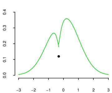
It follows that the distribution of $n^{1/2}(\hat{\theta}_{A}-\theta)$ consists of an atomic part given by

\left\{\Phi(n^{1/2}(-\theta+\mu_{n}))-\Phi(n^{1/2}(-\theta-\mu_{n}))\right\}\delta_{-n^{1/2}\theta},

(10)

where $\delta_{z}$ represents pointmass at the point $z$ , and an absolutely continuous part that has a Lebesgue density given by

	$\displaystyle 0.5\times\left\{\boldsymbol{1}(n^{1/2}\theta+x>0)\;\phi\left(z_{n,\theta}^{(2)}(x)\right)\;(1+t_{n,\theta}(x))\;+\;\right.$
	$\displaystyle\left.\boldsymbol{1}(n^{1/2}\theta+x<0)\;\phi\left(z_{n,\theta}^{(1)}(x)\right)\;(1-t_{n,\theta}(x))\right\},$		(11)

where $t_{n,\theta}(x)=0.5(n^{1/2}\theta+x)/\left(((n^{1/2}\theta+x)/2)^{2}+n\mu_{n}^{2}\right)^{1/2}$ . Figure 1 illustrates the shape of the finite-sample distribution of $n^{1/2}(\hat{\theta}_{A}-\theta)$ . Obviously, the distribution is highly non-normal.

Refer to caption — Figure 1: Distribution of $n^{1/2}(\hat{\theta}_{A}-\theta)$ for $n=10$ , $\theta=0.1$ , $\mu_{n}=0.05$ . The plot shows the density of the absolutely continuous part (11), as well as the total mass of the atomic part (10) located at $-n^{1/2}\theta=-0.32$ .

3.3.2 Asymptotic distributions

We next obtain the asymptotic distributions of $\hat{\theta}_{A}$ under general “moving parameter” asymptotics (i.e., asymptotics where the true parameter can depend on sample size), since – as already noted earlier – considering only fixed-parameter asymptotics may paint a very misleading picture of the behavior of the estimator. In fact, the results given below amount to a complete description of all possible accumulation points of the finite-sample distribution, cf. Remarks 7. Not surprisingly, the results in the conservative model selection case are different from the ones in the consistent model selection case.

Conservative case

The large-sample behavior of the distribution $F_{A,n,\theta_{n}}$ of $n^{1/2}(\hat{\theta}_{A}-\theta_{n})$ for the case when the estimator is tuned to perform conservative model selection is characterized in the following theorem.

Theorem 4

Assume $\mu_{n}\rightarrow 0$ and $n^{1/2}\mu_{n}\rightarrow\mathfrak{m}$ , $0\leq\mathfrak{m}<\infty$ . Suppose the true parameter $\theta_{n}\in\mathbb{R}$ satisfies $n^{1/2}\theta_{n}\rightarrow\nu\in\mathbb{R}\cup\{-\infty,\infty\}$ . Then, for $\nu\in\mathbb{R}$ , $F_{A,n,\theta_{n}}$ converges weakly to the distribution

\boldsymbol{1}(x+\nu\geq 0)\Phi\left(-{\frac{\nu-x}{2}}+\sqrt{({\frac{\nu+x}{2}})^{2}+\mathfrak{m}^{2}}\right)\\ +\boldsymbol{1}(x+\nu<0)\Phi\left(-{\frac{\nu-x}{2}}-\sqrt{({\frac{\nu+x}{2}})^{2}+\mathfrak{m}^{2}}\right).

If $|\nu|=\infty$ , then $F_{A,n,\theta_{n}}$ converges weakly to $\Phi$ , i.e., to a standard normal distribution.

The fixed-parameter asymptotic distribution can be obtained from Theorem 4 by setting $\theta_{n}\equiv\theta$ : For $\theta=0$ , we get

\boldsymbol{1}(x\geq 0)\;\Phi(x/2+\sqrt{(x/2)^{2}+\mathfrak{m}^{2}})+\boldsymbol{1}(x<0)\;\Phi(x/2-\sqrt{(x/2)^{2}+\mathfrak{m}^{2}}),

which coincides with the finite-sample distribution in (9) except for replacing $n^{1/2}\mu_{n}$ with its limit $\mathfrak{m}$ . However, for $\theta\neq 0$ , the resulting fixed-parameter asymptotic distribution is a standard normal distribution which clearly misrepresents the actual distribution (9). This disagreement is most pronounced in the statistically interesting case where $\theta$ is close to, but not equal to, zero (e.g., $\theta\sim n^{-1/2}$ ). In contrast, the distribution given in Theorem 4 much better captures the behavior of the finite-sample distribution also in this case because it coincides with the finite-sample distribution (9) except for the fact that $n^{1/2}\mu_{n}$ and $n^{1/2}\theta_{n}$ have settled down to their limiting values.

Consistent case

In this subsection we consider the case where the tuning parameter $\mu_{n}$ is chosen so that $\hat{\theta}_{A}$ performs consistent model selection, i.e. $\mu_{n}\rightarrow 0$ and $n^{1/2}\mu_{n}\rightarrow\infty$ .

Theorem 5

Assume that $\mu_{n}\rightarrow 0$ and $n^{1/2}\mu_{n}\rightarrow\infty$ . Suppose the true parameter $\theta_{n}\in\mathbb{R}$ satisfies $\theta_{n}/\mu_{n}\rightarrow\zeta$ for some $\zeta\in\mathbb{R}\cup\{-\infty,\infty\}$ .

1.

If $\zeta=0$ and $n^{1/2}\theta_{n}\rightarrow\nu\in\mathbb{R}$ , then $F_{A,n,\theta_{n}}$ converges weakly to the cdf $\boldsymbol{1}(\cdot\geq-\nu)$ .
2.

The total mass $F_{A,n,\theta_{n}}$ escapes to either $\infty$ or $-\infty$ for the following cases: If $-\infty<\zeta<0$ , or if $\zeta=0$ and $n^{1/2}\theta_{n}\rightarrow-\infty$ , or if $\zeta=-\infty$ and $n^{1/2}\mu_{n}^{2}/\theta_{n}\rightarrow-\infty$ , then $F_{A,n,\theta_{n}}(x)\rightarrow 0$ for every $x\in\mathbb{R}$ . If $0<\zeta<\infty$ , or if $\zeta=0$ and $n^{1/2}\theta_{n}\rightarrow\infty$ , or if $\zeta=\infty$ and $n^{1/2}\mu_{n}^{2}/\theta_{n}\rightarrow\infty$ , then $F_{A,n,\theta_{n}}(x)\rightarrow 1$ for every $x\in\mathbb{R}$ .
3.

If $\left|\zeta\right|=\infty$ and $n^{1/2}\mu_{n}^{2}/\theta_{n}\rightarrow r\in\mathbb{R}$ , then $F_{A,n,\theta_{n}}$ converges weakly to the cdf $\Phi(\cdot+r)$ .

The fixed-parameter asymptotic behavior of the adaptive LASSO estimator is obtained from Theorem 5 by setting $\theta_{n}\equiv\theta$ : For $\theta=0$ , the asymptotic distribution reduces to point-mass at $0$ , which coincides with the asymptotic distribution of the restricted maximum likelihood estimator. In the case of $\theta\neq 0$ , the asymptotic distribution is $\Phi(x+\rho/\theta)$ provided $n^{1/2}\mu_{n}^{2}\rightarrow\rho$ (with the obvious interpretation if $\left|\rho\right|=\infty$ ). That is, it is a shifted version of the asymptotic distribution of the unrestricted maximum likelihood estimator (the shift being infinitely large if $\left|\rho\right|=\infty$ ). Observe that (for $\left|\rho\right|<\infty$ ) the shift gets larger as $\left|\theta\right|$ , $\left|\theta\right|\neq 0$ , gets smaller. The ‘oracle’ property in the sense of Zou (2006) is hence satisfied if and only if $\rho=0$ , that is, if the tuning parameter additionally also satisfies $n^{1/4}\mu_{n}\rightarrow 0$ . This is precisely the condition imposed in Theorem 2 in Zou (2006) which establishes the ‘oracle’ property. [Note that $n^{1/4}\mu_{n}\rightarrow 0$ translates into the assumption $\lambda_{n}/n^{1/2}\rightarrow 0$ in Theorem 2 in Zou (2006).] If $n^{1/2}\mu_{n}^{2}\rightarrow\rho\neq 0$ , the adaptive LASSO estimator provides an example of an estimator that performs consistent model selection, but does not satisfy the ‘oracle’ property in the sense that for $\theta\neq 0$ its asymptotic distribution does not coincide with the asymptotic distribution of the unrestricted maximum likelihood estimator.

In any case, the ‘oracle’ property, which is guaranteed under the additional requirement $n^{1/4}\mu_{n}\rightarrow 0$ , carries little statistical meaning: Imposing the additional condition $n^{1/4}\mu_{n}\rightarrow 0$ still allows all three cases in Theorem 5 above to occur, showing that – notwithstanding the validity of the ‘oracle’ property – non-normal limiting distributions arise under a moving-parameter asymptotic framework. These latter distributions are in better agreement with the features exhibited by the finite-sample distribution (9), whereas the ‘oracle’ property always predicts a normal limiting distribution (a singular one in case $\theta=0$ ), showing that it does not capture essential features of the finite-sample distribution. In particular, the preceding theorem shows that the estimator is not uniformly $n^{1/2}$ -consistent as the sequence of finite-sample distributions of $n^{1/2}(\hat{\theta}_{A}-\theta_{n})$ is stochastically unbounded in some cases arising in Theorem 5. All this goes to show that the ‘oracle’ property, which is based on the pointwise asymptotic distribution only, paints a highly misleading picture of the behavior of the adaptive LASSO estimator and should not be taken at face value. See also Remark 10.

It transpires from Theorem 5 that $F_{A,n,\theta_{n}}$ converges weakly to the singular normal distribution $N(0,0)$ if $\theta_{n}=0$ for all $n$ , and to the standard normal $N(0,1)$ if $\theta_{n}$ satisfies $\left|\theta_{n}\right|/(n^{1/2}\mu_{n}^{2})\rightarrow\infty$ . Hence, if one, for example, allows as the parameter space for $\theta$ only the set $\Theta_{n}=\left\{\theta\in\mathbb{R}:\theta=0\text{ or }\left|\theta\right|>b_{n}\right\}$ where $b_{n}>0$ satisfies $b_{n}/(n^{1/2}\mu_{n}^{2})\rightarrow\infty$ , then the convergence of $F_{A,n,\theta_{n}}$ to the limiting distributions $N(0,0)$ and $N(0,1)$ , respectively, is uniform over $\Theta_{n}$ , i.e., the ‘oracle’ property holds uniformly over $\Theta_{n}$ . Does this line of reasoning restore the credibility of the ‘oracle’ property? We do not think so for the following reasons: The choice of $\Theta_{n}$ as the parameter space is highly artificial, depends on sample size as well as on the tuning parameter (and hence on the estimation procedure). Furthermore, in case $\Theta_{n}$ is adopted as the parameter space, the ‘forbidden’ set $\mathbb{R-}\Theta_{n}$ will always have a diameter that is of order larger than $n^{-1/2}$ ; in fact, it will always contain elements $\theta_{n}\neq 0$ such that $\theta_{n}$ would be correctly classified as non-zero with probability converging to one by the adaptive LASSO procedure used, i.e., $P_{n,\theta_{n}}(\hat{\theta}_{A}\neq 0)\rightarrow 1$ (to see this note that $\mathbb{R-}\Theta_{n}$ contains elements $\theta_{n}$ satisfying $\mathbb{\theta}_{n}/\mu_{n}\rightarrow\zeta$ with $\left|\zeta\right|>1$ and use Proposition 1). This shows that adopting $\Theta_{n}$ as the parameter space rules out values of $\theta$ that are substantially different from zero, and not only values of $\theta$ that are difficult to statistically distinguish from zero; consequently the ‘forbidden’ set is sizable. Summarizing, there appears to be little reason why $\Theta_{n}$ would be a natural choice of parameter space, especially in the context of model selection where interest naturally focusses on the neighborhood of zero. We therefore believe that using $\Theta_{n}$ as the parameter space is hardly supported by statistical reasoning but is more reflective of a search for conditions that are favorable to the ‘oracle’ property.

As mentioned above, Theorem 5 shows, in particular, that $\hat{\theta}_{A}$ is not uniformly $n^{1/2}$ -consistent. This prompts the question of the behavior of the distribution of $c_{n}(\hat{\theta}_{A}-\theta_{n})$ under a sequence of norming constants $c_{n}$ that are $o(n^{1/2})$ . Inspection of the proof of Theorem 5 reveals that the stochastic unboundedness phenomenon persists if $c_{n}$ is $o(n^{1/2})$ but is of order larger than $\mu_{n}^{-1}$ . For $c_{n}=O(\mu_{n}^{-1})$ , we always have stochastic boundedness by Theorem 2. Hence, the uniform convergence rate of $\hat{\theta}_{A}$ is seen to be $\mu_{n}$ which is slower than $n^{-1/2}$ . The precise limit distributions of the estimator under the scaling $c_{n}\sim\mu_{n}^{-1}$ is obtained in the next theorem. [The case $c_{n}=o(\mu_{n}^{-1})$ is trivial since then these limits are always pointmass at zero in view of Theorem 2.³³ 3 There is no loss in generality here in the sense that the general case where $c_{n}=O(\mu_{n}^{-1})$ holds can – by passing to subsequences – always be reduced to the cases where $c_{n}\sim\mu_{n}^{-1}$ or $c_{n}=o(\mu_{n}^{-1})$ holds.] A consequence of the next theorem is that with such a scaling the pointwise limiting distributions always degenerate to pointmass at zero. This points to something of a dilemma with the adaptive LASSO estimator when tuned to perform consistent model selection: If we scale the estimator by $\mu_{n}^{-1}$ , i.e., by the ‘right’ uniform rate, the pointwise limiting distributions degenerate to pointmass at zero. If we scale the estimator by $n^{1/2}$ , which is the ‘right’ pointwise rate (at least if $n^{1/4}\mu_{n}\rightarrow 0$ ), then we end up with stochastically unbounded sequences of distributions under a moving parameter asymptotic framework (for certain sequences $\theta_{n}$ ).

Let $G_{A,n,\theta}$ stand for the finite-sample distribution of $\mu_{n}^{-1}(\hat{\theta}_{A}-\theta)$ under $P_{n,\theta}$ . Clearly, $G_{A,n,\theta}(x)=F_{A,n,\theta}(n^{1/2}\mu_{n}x)$ . The limits of this distribution under ‘moving parameter’ asymptotics are given in the subsequent theorem. It turns out that the limiting distributions are always pointmasses, however, not always located at zero.

Theorem 6

Assume that $\mu_{n}\rightarrow 0$ , $n^{1/2}\mu_{n}\rightarrow\infty$ , and that $\theta_{n}/\mu_{n}\rightarrow\zeta$ for some $\zeta\in\mathbb{R}\cup\{-\infty,\infty\}$ .

1.

If $|\zeta|<1$ , then $G_{A,n,\theta_{n}}$ converges weakly to the cdf $\boldsymbol{1}(\cdot\geq-\zeta)$ .
2.

If $1\leq|\zeta|<\infty$ , then $G_{A,n,\theta_{n}}$ converges weakly the cdf $\boldsymbol{1}(\cdot\geq-1/\zeta)$ .
3.

If $|\zeta|=\infty$ , then $G_{A,n,\theta_{n}}$ converges weakly to the cdf $\boldsymbol{1}(\cdot\geq 0)$ .

3.3.3 Some Remarks

Remark 7

Theorems 4 and 5 actually completely describe all accumulation points of the finite-sample distribution of $n^{1/2}(\hat{\theta}_{A}-\theta_{n})$ without any condition on the sequence of parameters $\theta_{n}$ . To see this, just apply the theorems to subsequences and note that by compactness of $\mathbb{R}\cup\{-\infty,\infty\}$ we can select from every subsequence a further subsequence such that the relevant quantities like $n^{1/2}\theta_{n}$ , $\theta_{n}/\mu_{n}$ , and $n^{1/2}\mu_{n}^{2}/\theta_{n}$ converge in $\mathbb{R}\cup\{-\infty,\infty\}$ along this further subsequence. A similar comment also applies to Theorem 6.

Remark 8

As a point of interest we note that the full complexity of the possible limiting distributions in Theorems 4, 5, and 6 already arises if we restrict the sequences $\theta_{n}$ to a bounded neighborhood of zero. Hence, the phenomena described by the above theorems are of a local nature, and are not tied in any way to the unboundedness of the parameter space.

Remark 9

In case the estimator is tuned to perform consistent model selection, it is mainly the behavior of $\theta_{n}/\mu_{n}$ that governs the form of the limiting distributions in Theorems 5 and 6. Note that $\theta_{n}/\mu_{n}$ is of smaller order than $n^{1/2}\theta_{n}$ because $n^{1/2}\mu_{n}\rightarrow\infty$ in the consistent case. Hence, an analysis relying only on the classical local asymptotics based on perturbations of $\theta$ of the order of $n^{-1/2}$ does not properly reveal all possible limits of the finite-sample distributions in that case. [This is in contrast to the conservative case, where classical local asymptotics reveal all possible limit distributions.]

Remark 10

The mathematical reason for the failure of the pointwise asymptotic distributions to capture the behavior of the finite-sample distributions well is that the convergence of the latter to the former is not uniform in the underlying parameter $\theta\in\mathbb{R}$ . See Leeb & Pötscher (2003), Leeb & Pötscher (2005) for more discussion in the context of post-model-selection estimators.

Remark 11

The theoretical analysis has been restricted to the case of orthogonal regressors. In the case of correlated regressors we can expect to see similar phenomena (e.g., non-normality of finite-sample cdfs, non-uniformity problems, etc.), although details will be different. Evidence for this is provided by the simulation study presented in Section 4, by corresponding theoretical results for a class of post-model-selection estimators (Leeb & Pötscher (2003), Leeb & Pötscher (2006a), Leeb & Pötscher (2008b)) in the correlated regressor case as well as by general results on estimators possessing the sparsity property (Leeb & Pötscher (2008a), Pötscher (2007)).

3.4 Impossibility results for estimating the distribution of the adaptive LASSO

Since the cdf $F_{A,n,\theta}$ of $n^{1/2}(\hat{\theta}_{A}-\theta)$ depends on the unknown parameter, as shown in Section 3.3.1, one might be interested in estimating this cdf. We show that this is an intrinsically difficult estimation problem in the sense that the cdf cannot be estimated in a uniformly consistent fashion. In the following, we provide large-sample results that cover both consistent and conservative choices of the tuning parameter, as well as finite-sample results that hold for any choice of tuning parameter. For related results in different contexts see Leeb & Pötscher (2006a), Leeb & Pötscher (2006b), Leeb & Pötscher (2008a), Pötscher (2006), Pötscher & Leeb (2007).

It is straightforward to construct consistent estimators for the distribution $F_{A,n,\theta}$ of the (centered and scaled) estimator $\hat{\theta}_{A}$ . One popular choice is to use subsampling or the $m$ out of $n$ bootstrap with $m/n\rightarrow 0$ . Another possibility is to use the pointwise large-sample limit distributions derived in Section 3.3.2 together with a properly chosen pre-test of the hypothesis $\theta=0$ versus $\theta\neq 0$ . Because the pointwise large-sample limit distribution takes only two different functional forms depending on whether $\theta=0$ or $\theta\neq 0$ , one can perform a pre-test that rejects the hypothesis $\theta=0$ in case $|\bar{y}|>n^{-1/4}$ , say, and estimate the finite-sample distribution by that large-sample limit formula that corresponds to the outcome of the pre-test;⁴⁴ 4 In the conservative case, the asymptotic distribution can also depend on $\mathfrak{m}$ which is then to be replaced by $n^{1/2}\mu_{n}$ . the test’s critical value $n^{-1/4}$ ensures that the correct large-sample limit formula is selected with probability approaching one as sample size increases. However, as we show next, any consistent estimator of the cdf $F_{A,n,\theta}$ is necessarily badly behaved in a worst-case sense.

Theorem 12

Let $\mu_{n}$ be a sequence of tuning parameters such that $\mu_{n}\rightarrow 0$ and $n^{1/2}\mu_{n}\rightarrow\mathfrak{m}$ with $0\leq\mathfrak{m}\leq\infty$ . Let $t\in\mathbb{R}$ be arbitrary. Then every consistent estimator $\hat{F}_{n}(t)$ of $F_{A,n,\theta}(t)$ satisfies

\lim_{n\rightarrow\infty}\sup_{|\theta|<c/n^{1/2}}P_{n,\theta}\left(\left|\hat{F}_{n}(t)-F_{A,n,\theta}(t)\right|\;>\;\varepsilon\right)\;\;=\;\;1

for each $\varepsilon<(\Phi(t+\mathfrak{m})-\Phi(t-\mathfrak{m}))/2$ and each $c>\left|t\right|$ . In particular, no uniformly consistent estimator for $F_{A,n,\theta}(t)$ exists.

We stress that the above result also applies to any kind of bootstrap- or subsampling-based estimator of the cdf $F_{A,n,\theta}$ whatsoever, since the results in Leeb & Pötscher (2006b) on which the proof of Theorem 12 rests apply to arbitrary randomized estimators, cf. Lemma 3.6 in Leeb & Pötscher (2006b). The same applies to Theorems 13 and 14 that follow.

Loosely speaking, Theorem 12 states that any consistent estimator for the cdf $F_{A,n,\theta}$ suffers from an unavoidable worst-case error of at least $\varepsilon$ with $\varepsilon<(\Phi(t+\mathfrak{m})-\Phi(t-\mathfrak{m}))/2$ . The error range, i.e., $(\Phi(t+\mathfrak{m})-\Phi(t-\mathfrak{m}))/2$ , is governed by the limit $\mathfrak{m}=\lim_{n}n^{1/2}\mu_{n}$ . In case the estimator is tuned to be consistent, i.e., in case $\mathfrak{m}=\infty$ , the error range equals $1/2$ , and the phenomenon is most pronounced. If the estimator is tuned to be conservative so that $\mathfrak{m}<\infty$ , the error range is less than $1/2$ but can still be substantial. Only in case $\mathfrak{m}=0$ the error range equals zero, and the condition $\varepsilon<(\Phi(t+\mathfrak{m})-\Phi(t-\mathfrak{m}))/2$ in Theorem 12 leads to a trivial conclusion. This is, however, not surprising as then the resulting estimator is uniformly asymptotically equivalent to the unrestricted maximum likelihood estimator $\bar{y}$ , cf. Remark 3.

A similar non-uniformity phenomenon as described in Theorem 12 for consistent estimators $\hat{F}_{n}(t)$ also occurs for not necessarily consistent estimators. For such arbitrary estimators we find in the following that the phenomenon can be somewhat less pronounced, in the sense that the lower bound is now $1/2$ instead of $1$ , cf. (13) below. The following theorem gives a large-sample limit result that parallels Theorem 12, as well as a finite-sample result, both for arbitrary (and not necessarily consistent) estimators of the cdf.

Theorem 13

Let $0<\mu_{n}<\infty$ and let $t\in\mathbb{R}$ be arbitrary. Then every estimator $\hat{F}_{n}(t)$ of $F_{A,n,\theta}(t)$ satisfies

\sup_{|\theta|<c/n^{1/2}}P_{n,\theta}\left(\left|\hat{F}_{n}(t)-F_{A,n,\theta}(t)\right|\;>\;\varepsilon\right)\;\;\geq\;\;\frac{1}{2}

(12)

for each $\varepsilon<(\Phi(t+n^{1/2}\mu_{n})-\Phi(t-n^{1/2}\mu_{n}))/2$ , for each $c>|t|$ , and for each fixed sample size $n$ . If $\mu_{n}$ satisfies $\mu_{n}\rightarrow 0$ and $n^{1/2}\mu_{n}\rightarrow\mathfrak{m}$ as $n\rightarrow\infty$ with $0\leq\mathfrak{m}\leq\infty$ , we thus have

\liminf_{n\rightarrow\infty}\inf_{\hat{F}_{n}(t)}\sup_{|\theta|<c/n^{1/2}}P_{n,\theta}\left(\left|\hat{F}_{n}(t)-F_{A,n,\theta}(t)\right|\;>\;\varepsilon\right)\;\;\geq\;\;\frac{1}{2}

(13)

for each $\varepsilon<(\Phi(t+\mathfrak{m})-\Phi(t-\mathfrak{m}))/2$ and for each $c>|t|$ , where the infimum in (13) extends over all estimators $\hat{F}_{n}(t)$ .

The finite-sample statement in Theorem 13 clearly reveals how the estimability of the cdf of the estimator depends on the tuning parameter $\mu_{n}$ : A larger value of $\mu_{n}$ , which results in a ‘more sparse’ estimator in view of (5), directly corresponds to a larger range $(\Phi(t+n^{1/2}\mu_{n})-\Phi(t-n^{1/2}\mu_{n}))/2$ for the error $\varepsilon$ within which any estimator $\hat{F}_{n}(t)$ performs poorly in the sense of (12). In large samples, the limit $\mathfrak{m}=\lim_{n\rightarrow\infty}n^{1/2}\mu_{n}$ takes the role of $n^{1/2}\mu_{n}$ .

An impossibility result paralleling Theorem 13 for the cdf $G_{A,n,\theta}(t)$ of $\mu_{n}^{-1}(\hat{\theta}_{A}-\theta)$ is given next.

Theorem 14

Let $0<\mu_{n}<\infty$ and let $t\in\mathbb{R}$ be arbitrary. Then every estimator $\hat{G}_{n}(t)$ of $G_{A,n,\theta}(t)$ satisfies

\sup_{|\theta|<c\mu_{n}}P_{n,\theta}\left(\left|\hat{G}_{n}(t)-G_{A,n,\theta}(t)\right|\;>\;\varepsilon\right)\quad\geq\quad\frac{1}{2}

(14)

for each $\varepsilon<(\Phi(n^{1/2}\mu_{n}(t+1))-\Phi(n^{1/2}\mu_{n}(t-1)))/2$ , for each $c>|t|$ , and for each fixed sample size $n$ . If $\mu_{n}$ satisfies $\mu_{n}\rightarrow 0$ and $n^{1/2}\mu_{n}\rightarrow\infty$ as $n\rightarrow\infty$ , we thus have for each $c>|t|$

\liminf_{n\rightarrow\infty}\inf_{\hat{G}_{n}(t)}\sup_{|\theta|<c\mu_{n}}P_{n,\theta}\left(\left|\hat{G}_{n}(t)-G_{A,n,\theta}(t)\right|\;>\;\varepsilon\right)\quad\geq\quad\frac{1}{2}

(15)

for each $\varepsilon<1/2$ if $\left|t\right|<1$ and for each $\varepsilon<1/4$ if $\left|t\right|=1$ , where the infimum in (15) extends over all estimators $\hat{G}_{n}(t)$ .

This result shows, in particular, that no uniformly consistent estimator exists for $G_{A,n,\theta}(t)$ in case $\left|t\right|\leq 1$ (not even over compact subsets of $\mathbb{R}$ containing the origin). In view of Theorem 6, we see that for $t>1$ we have $\sup_{\theta\in\mathbb{R}}\left|G_{A,n,\theta}(t)-1\right|\rightarrow 0$ as $n\rightarrow\infty$ , hence $\hat{G}_{n}(t)=1$ is trivially a uniformly consistent estimator in this case. Similarly, for $t<-1$ we have $\sup_{\theta\in\mathbb{R}}\left|G_{A,n,\theta}(t)\right|\rightarrow 0$ as $n\rightarrow\infty$ , hence $\hat{G}_{n}(t)=0$ is trivially a uniformly consistent estimator in this case.

4 Some Monte Carlo Results

We provide simulation results for the finite-sample distribution of the adaptive LASSO estimator in the case of non-orthogonal regressors to complement our theoretical findings for the orthogonal case. We present our results by showing the marginal distribution for each component of the centered and scaled estimator. Not surprisingly, the graphs exhibit the same highly non-normal features of the corresponding finite-sample distribution of the estimator derived in Section 3.3 for the case of orthogonal regressors.

The simulations were carried out the following way. We consider 1000 repetitions of $n$ simulated data points from the model (1) with $\sigma^{2}=1$ and $X$ such that $X^{\prime}X=n\Omega$ with $\Omega_{ij}=0.5^{|i-j|}$ for $i,j=1,\dots,k$ . More concretely, $X$ was partitioned into $d=n/k$ blocks of size $k\times k$ (where $d$ is assumed to be integer) and each of these blocks was set equal to $k^{1/2}L$ , with $LL^{\prime}=\Omega$ , the Cholesky factorization of $\Omega$ . We used $k=4$ regressors and various values of the true parameter $\theta$ given by $\theta=(3,1.5,\gamma n^{-1/2},\gamma n^{-1/2})^{\prime}$ where $\gamma=0,1,2$ . This model with $\theta=(3,1.5,0,0)^{\prime}$ (i.e., $\gamma=0$ ) is a downsized version of a model considered in Monte Carlo studies in Tibshirani (1996), Fan & Li (2001), and Zou (2006). For apparent reasons it is of interest to investigate the performance of the estimator not only at a single parameter value, but also at other (neighboring) points in the parameter space. The cases with $\gamma\neq 0$ , represent the statistically interesting case where some components of the true parameter value are close to but not equal to zero.

For each simulation, we computed the adaptive LASSO estimator $\hat{\theta}_{A}$ using the LARS package of Efron et al. (2004) in R. Each component of the estimator was centered and scaled, i.e., $C_{jj}^{-1/2}(\hat{\theta}_{A,j}-\theta_{j})$ was computed, where $C=(n\Omega)^{-1}$ . The tuning parameter $\mu_{n}$ was chosen in two different ways. In the first case, it was set to the fixed value of $\mu_{n}=n^{-1/3}$ , a choice that corresponds to consistent model selection and additionally satisfies the condition $n^{1/4}\mu_{n}\rightarrow 0$ required in Zou (2006) to obtain the ’oracle’ property. In the second case, in each simulation the tuning parameter was selected to minimize a mean-squared prediction error obtained through $K$ -fold cross-validation (which can be computed using the LARS package, in our case with $K=10$ ).

The results for both choices of the tuning parameters, for $n=100$ , and $\gamma=0,1,2$ are shown in Figures 2-7 below. For each component of the estimator, the discrete component of the distribution corresponding to the zero values of the $j$ -th component of the estimator $\hat{\theta}_{A,j}$ (appearing at $-C_{jj}^{-1/2}\theta_{j}$ for the centered and scaled estimator) is represented by a dot drawn at the height of the corresponding relative frequency. The histogram formed from the remaining values of $C_{jj}^{-1/2}(\hat{\theta}_{A,j}-\theta_{j})$ was then smoothed by the kernel smoother available in R, resulting in the curves representing the density of the absolutely continuous part of the finite-sample distribution of $C_{jj}^{-1/2}(\hat{\theta}_{A,j}-\theta_{j})$ . Naturally, in these plots the density was rescaled by the appropriate relative frequency of the estimator not being equal to zero.

We first discuss the case where the tuning parameter is set at the fixed value $\mu_{n}=n^{-1/3}$ . For $\gamma=0$ , i.e., the case where the last two components of the true parameter are identically zero, Figure 2 shows that the adaptive LASSO estimator finds the zero components in $\theta=(3,1.5,0,0)^{\prime}$ with probability close to one (i.e., the distributions of $C_{jj}^{-1/2}(\hat{\theta}_{A,j}-\theta_{j})$ , $j=3,4$ , practically coincide with pointmass at $0$ ). Furthermore, the distributions of the first two components seem to somewhat resemble normality. The outcome in this case is hence roughly in line with what the ’oracle’ property predicts. This is due to the fact that the components of $\theta$ are either zero or large (note that $C_{jj}^{-1/2}\theta_{j}$ is approximately equal to $26$ and $12$ , respectively, for $j=1,2$ ). The results are quite different for the cases $\gamma=1$ and $\gamma=2$ (Figures 3 and 4), which represent the case where some of the components of the parameter vector $\theta$ are large and some are different from zero but small (note that $C_{33}^{-1/2}\theta_{3}\approx 0.77\gamma$ and $C_{44}^{-1/2}\theta_{4}\approx 0.87\gamma$ ). In both cases the distributions of $C_{jj}^{-1/2}(\hat{\theta}_{A,j}-\theta_{j})$ , $j=3,4$ , are a mixture of an atomic part and an absolutely continuous part, both shifted to the left of the origin. Furthermore, the absolutely continuous part appears to be highly non-normal. This is perfectly in line with the theoretical results obtained in Section 3.3. It once again demonstrates that the ’oracle’ property gives a misleading impression of the actual performance of the estimator.

In the case where the tuning parameter is chosen by cross-validation, a similar picture emerges, except for the fact that in case $\gamma=0$ the adaptive LASSO estimator now finds the zero component less frequently, cf. Figure 5. [In fact, the probability of finding a zero value of $\hat{\theta}_{A,j}$ for $j=3,4$ is smaller in the cross-validated case regardless of the value of $\gamma$ considered.] The reason for this is that the tuning parameters obtained through cross-validation were typically found to be smaller than $n^{-1/3}$ , resulting in an estimator $\hat{\theta}_{A}$ that acts more like a conservative rather than a consistent model selection procedure. [This is in line with theoretical results in Leng et al. (2006), see also Leeb & Pötscher (2008b).] In agreement with the theoretical results in Section 3.3, the absolutely continuous components of the distributions of $C_{jj}^{-1/2}(\hat{\theta}_{A,j}-\theta_{j})$ are now typically highly non-normal, especially for $j=3,4$ , cf. Figures 5-7. [Note that cross-validation leads to a data-depending tuning parameter $\mu_{n}$ , a situation that is strictly speaking not covered by the theoretical results.]

We have also experimented with other values of $\theta$ such as $\theta=(3,1.5,\gamma n^{-1/2},0)^{\prime}$ or $\theta=(3,1.5,0,\gamma n^{-1/2}\,)^{\prime}$ , other values of $\gamma$ and other sample sizes such as $n=60$ or $200$ . The results were found to be qualitatively the same.

5 Conclusion

We have studied the distribution of the adaptive LASSO estimator, a penalized least squares estimator introduced in Zou (2006), in finite-samples as well as in the large-sample limit. The theoretical study assumes an orthogonal regression model. The finite-sample distribution was found to be a mixture of a singular normal distribution and an absolutely continuous distribution, which is non-normal. The large-sample limit of the distributions depends on the choice of the estimator’s tuning parameter, and we can distinguish two cases:

In the first case the tuning is such that the estimator acts as a conservative model selector. In this case, the adaptive LASSO estimator is found to be uniformly $n^{1/2}$ -consistent. We also show that fixed-parameter asymptotics (where the true parameter remains fixed while sample size increases) only partially reflect the actual behavior of the distribution whereas “moving-parameter” asymptotics (where the true parameter may depend on sample size) gives a more accurate picture. The moving-parameter analysis shows that the distribution may be highly non-normal irrespective of sample size, in particular, in the statistically interesting case where the true parameter is close (in an appropriate sense) to a lower-dimensional submodel. This also implies that the finite-sample phenomena that we have observed can occur at any sample size.

In the second case, where the estimator is tuned to perform consistent model selection, again fixed-parameter asymptotics do not capture the whole range of large-sample phenomena that can occur. With ‘moving parameter’ asymptotics, we have shown that the distribution of these estimators can again be highly non-normal, even in large samples. In addition, we have found that the observed finite-sample phenomena not only can persist but actually can be more pronounced for larger sample sizes. For example, the distribution of the estimator (properly centered and scaled by $n^{1/2}$ ) can diverge in the sense that all its mass escapes to either $+\infty$ or $-\infty$ . In fact, we have established that the uniform convergence rate of the adaptive LASSO estimator is slower than $n^{-1/2}$ in the consistent model selection case. These findings are especially important as the adaptive LASSO estimator has been shown in Zou (2006) to possess an ’oracle’ property (under an additional assumption on the tuning parameter), which promises a convergence rate of $n^{-1/2}$ and a normal distribution in large samples. However, the ’oracle’ property is based on a fixed-parameter asymptotic argument which, as our results show, gives highly misleading results.

The findings mentioned above are based on a theoretical analysis (Section 3) of the adaptive LASSO estimator in an orthogonal linear regression model. The orthogonality restriction is removed in the Monte Carlo analysis in Section 4. The results from this simulation study confirm the theoretical results.

Finally, we have studied the problem of estimating the cdf of the (centered and scaled) adaptive LASSO estimator. We have shown that this cdf cannot be estimated in a uniformly consistent fashion, even though pointwise consistent estimators can be constructed with relative ease.

We would like to stress that our results should not be read as a condemnation of the adaptive LASSO estimator, but as a warning that the distributional properties of this estimator are quite intricate and complex.

Appendix A Appendix

Proof of Theorem 2: Since (7) implies (6), it suffices to prove the former. For this, it is instructive to write $\hat{\theta}_{A}$ in terms of the hard-thresholding estimator $\hat{\theta}_{H}$ as defined in Pötscher & Leeb (2007) (with $\eta_{n}=\mu_{n}$ ) by observing that

\hat{\theta}_{A}=\hat{\theta}_{H}-\mathop{\mathrm{s}ign}(\hat{\theta}_{H})\mu_{n}^{2}/|\bar{y}|.

Here $\mathop{\mathrm{s}ign}(x)=-1,0,1$ depending on whether $x<0,=0,>0$ . Since $\hat{\theta}_{H}$ satisfies (7) as is shown in Theorem 2 in Pötscher & Leeb (2007), it suffices to consider

$\displaystyle\sup_{\theta\in\mathbb{R}}P_{n,\theta}(a_{n}\|\hat{\theta}_{H}-\hat{\theta}_{A}\|>M)$	$\displaystyle=$	$\displaystyle\sup_{\theta\in\mathbb{R}}P_{n,\theta}(a_{n}\mu_{n}^{2}/\|\bar{y}\|>M,\hat{\theta}_{H}\neq 0)$
	$\displaystyle=$	$\displaystyle\sup_{\theta\in\mathbb{R}}P_{n,\theta}(a_{n}\mu_{n}^{2}/\|\bar{y}\|>M,\|\bar{y}\|>\mu_{n})$
	$\displaystyle\leq$	$\displaystyle\boldsymbol{1}(a_{n}\mu_{n}>M).$

Since $a_{n}\mu_{n}\leq 1$ , the right-hand side in the above expression equals zero for any $M>1$ . $\blacksquare$

Proposition 15

Let $\theta_{n}\in\mathbb{R}$ and $0<\mu_{n}<\infty$ . If $\theta_{n}/\mu_{n}\rightarrow-\infty$ and $n^{1/2}\theta_{n}\rightarrow-\infty$ , then $z_{n,\theta_{n}}^{(1)}(x)-x\sim n^{1/2}\mu_{n}^{2}/\theta_{n}$ as $n\rightarrow\infty$ for every $x\in\mathbb{R}$ . If $\theta_{n}/\mu_{n}\rightarrow\infty$ and $n^{1/2}\theta_{n}\rightarrow\infty$ , then $z_{n,\theta_{n}}^{(2)}(x)-x\sim n^{1/2}\mu_{n}^{2}/\theta_{n}$ for every $x\in\mathbb{R}$ .

Proof. We prove the first claim. We can write

	$\displaystyle z_{n,\theta_{n}}^{(1)}(x)-x$	$\displaystyle=$	$\displaystyle-(n^{1/2}\theta_{n}+x)/2-\sqrt{((n^{1/2}\theta_{n}+x)/2)^{2}+n\mu_{n}^{2}}$
		$\displaystyle=$	$\displaystyle n^{1/2}\alpha_{n}(x)\left\{-1+\sqrt{1+(\mu_{n}/\alpha_{n}(x))^{2}}\right\}$

with $n^{1/2}\alpha_{n}(x)=(n^{1/2}\theta_{n}+x)/2$ where the last equality holds for large $n$ since $n^{1/2}\alpha_{n}(x)<0$ eventually. Through an expansion of $\sqrt{1+z}$ about zero, we obtain

	$\displaystyle z_{n,\theta_{n}}^{(1)}(x)-x$	$\displaystyle=$	$\displaystyle n^{1/2}(\mu_{n}^{2}/\alpha_{n}(x))(1+\bar{z}_{n})^{-1/2}/2$
		$\displaystyle=$	$\displaystyle(n^{1/2}\mu_{n}^{2}/\theta_{n})(1+x/(n^{1/2}\theta_{n}))^{-1}(1+\bar{z}_{n})^{-1/2},$

with $0\leq\bar{z}_{n}\leq(\mu_{n}/\alpha_{n}(x))^{2}$ . Note that $\mu_{n}/\alpha_{n}(x)=2(\mu_{n}/\theta_{n})(1+x/(n^{1/2}\theta_{n}))^{-1}\rightarrow 0$ , and hence $\bar{z}_{n}\rightarrow 0$ holds. The claim now follows. The second claim is proved analogously.

Proof of Theorem 4: We derive the corresponding asymptotic distributions by studying the limit behavior of (9) with $\theta$ replaced by $\theta_{n}$ . If $\nu\in\mathbb{R}$ the result immediately follows, since $F_{A,n,\theta_{n}}(x)$ converges to the limit given above for every $x\neq-\nu$ as a consequence of (8) and $n^{1/2}\theta_{n}\rightarrow\nu$ . For the case $\nu=\infty$ , note that the indicator function of the first term in (9) goes to $1$ for every $x\in\mathbb{R}$ , whereas the second one goes to $0$ . Furthermore, we clearly have $\theta_{n}/\mu_{n}\rightarrow\infty$ since $0\leq\mathfrak{m}<\infty$ holds. Therefore we can apply Proposition 15 to find that $z_{n,\theta_{n}}^{(2)}(x)\rightarrow x$ since $n^{1/2}\mu_{n}^{2}/\theta_{n}=n^{1/2}\mu_{n}(\mu_{n}/\theta_{n})\rightarrow\mathfrak{m}\cdot 0=0$ . This implies that $F_{A,n,\theta}(x)\rightarrow\Phi(x)$ for all $x\in\mathbb{R}$ in case $\nu=\infty$ . A similar argument can be made to prove the claim for $\nu=-\infty$ . $\blacksquare$

Proof of Theorem 5: If $\left|\zeta\right|<1$ , Proposition 1 shows that the total mass of the atomic part (10) of the distribution $F_{A,n,\theta_{n}}$ goes to $1$ ; furthermore, the location of the atomic part, i.e., $-n^{1/2}\theta_{n}$ , then converges to $-\nu\in\mathbb{R}$ or to $\pm\infty$ . This proves the theorem in case $\left|\zeta\right|<1$ . We prove the remaining cases by inspecting the limit behavior of (9), again with $\theta_{n}$ replacing $\theta$ . To derive the limits for $1\leq\left|\zeta\right|\leq\infty$ , note that $n^{1/2}\theta_{n}\rightarrow\mathop{\mathrm{s}ign}(\zeta)\,\infty$ , so that by assessing the limit of the indicator functions in (9), it can easily be seen that $F_{A,n,\theta_{n}}(x)$ converges to the limit of $\Phi(z_{n,\theta_{n}}^{(2)}(x))$ for $\zeta>0$ and to the limit of $\Phi(z_{n,\theta_{n}}^{(1)}(x))$ for $\zeta<0$ . Elementary calculations show that $z_{n,\theta_{n}}^{(2)}(x)\rightarrow\infty$ for $1\leq\zeta<\infty$ and that $z_{n,\theta_{n}}^{(1)}(x)\rightarrow-\infty$ for $-\infty<\zeta\leq-1$ . As a consequence of Proposition 15, also $z_{n,\theta_{n}}^{(2)}(x)\rightarrow\infty$ if $\zeta=\infty$ and $n^{1/2}\mu_{n}^{2}/\theta_{n}\rightarrow\infty$ ; similarly, $z_{n,\theta_{n}}^{(1)}(x)\rightarrow-\infty$ if $\zeta=-\infty$ and $n^{1/2}\mu_{n}^{2}/\theta_{n}\rightarrow-\infty$ . This then proves the remaining cases in part 2. Under the assumptions of part 3, an application of Proposition 15 gives that $z_{n,\theta_{n}}^{(2)}(x)\rightarrow x+r$ if $\zeta=\infty$ and that $z_{n,\theta_{n}}^{(1)}(x)\rightarrow x+r$ if $\zeta=-\infty$ , which then proves part 3. $\blacksquare$

Proof of Theorem 6: To prove part 1, observe that Proposition 1 implies $\lim_{n\rightarrow\infty}P_{n,\theta_{n}}(\hat{\theta}_{A}=0)=1$ for $|\zeta|<1$ . This entails

	$\displaystyle\lim_{n\rightarrow\infty}P_{n,\theta_{n}}(\mu_{n}^{-1}(\hat{\theta}_{A}-\theta_{n})\leq x)$	$\displaystyle=\lim_{n\rightarrow\infty}P_{n,\theta_{n}}(\mu_{n}^{-1}(\hat{\theta}_{A}-\theta_{n})\leq x,\,\hat{\theta}_{A}=0)$
		$\displaystyle=\lim_{n\rightarrow\infty}\boldsymbol{1}(-\theta_{n}/\mu_{n}\leq x)=\boldsymbol{1}(x\geq-\zeta)$

for $x\neq-\zeta$ , which establishes part 1. Next, observe that

	$\displaystyle G_{A,n,\theta_{n}}(x)$	$\displaystyle=$
	$\displaystyle\boldsymbol{1}(\theta_{n}/\mu_{n}$	$\displaystyle+x\geq 0)\Phi(w_{n,\theta_{n}}^{(2)}(x))+\boldsymbol{1}(\theta_{n}/\mu_{n}+x<0)\Phi(w_{n,\theta_{n}}^{(1)}(x))$		(16)

where $w_{n,\theta_{n}}^{(1)}(x)$ and $w_{n,\theta_{n}}^{(2)}(x)$ with $w_{n,\theta_{n}}^{(1)}(x)\leq w_{n,\theta_{n}}^{(2)}(x)$ are given by

n^{1/2}\mu_{n}\left\{(-\theta_{n}/\mu_{n}+x)\pm\sqrt{(\theta_{n}/\mu_{n}+x)^{2}+4}\right\}/2.

(17)

Under the conditions of part 2, the first indicator function in (16) tends to $1$ for $x>-\zeta$ and to $0$ for $x<-\zeta$ . Consequently, $G_{A,n,\theta_{n}}(x)$ converges to $\lim_{n\rightarrow\infty}\Phi(w_{n,\theta_{n}}^{(2)}(x))$ if $x>-\zeta$ , and to $\lim_{n\rightarrow\infty}\Phi(w_{n,\theta_{n}}^{(1)}(x))$ if $x<-\zeta$ (provided the limits exist). Elementary calculations show that for $\zeta\geq 1$ we have $w_{n,\theta_{n}}^{(1)}(x)\rightarrow-\infty$ for all $x\in\mathbb{R}$ , $w_{n,\theta_{n}}^{(2)}(x)\rightarrow-\infty$ for $x<-1/\zeta$ , and $w_{n,\theta_{n}}^{(2)}(x)\rightarrow\infty$ for $x>-1/\zeta$ . For $\zeta\leq-1$ we obtain $w_{n,\theta_{n}}^{(1)}(x)\rightarrow-\infty$ for $x<-1/\zeta$ , $w_{n,\theta_{n}}^{(1)}(x)\rightarrow\infty$ for $x>-1/\zeta$ , and $w_{n,\theta_{n}}^{(2)}(x)\rightarrow\infty$ for all $x\in\mathbb{R}$ . Consequently, for $x\neq-\zeta$ , we find $G_{A,n,\theta_{n}}(x)\rightarrow 0$ for $x<-1/\zeta$ and $G_{A,n,\theta_{n}}(x)\rightarrow 1$ for $x>-1/\zeta$ . If $\left|\zeta\right|=1$ , the result in part 2 follows. If $\left|\zeta\right|>1$ , convergence of $G_{A,n,\theta_{n}}(-\zeta)$ to the proper limit follows from monotonicity of $G_{A,n,\theta_{n}}$ and the fact that $x=-\zeta$ is a continuity point of the limit distribution. This then completes the proof of part 2.

For part 3 we consider first the case $\zeta=\infty$ . Clearly, $G_{A,n,\theta_{n}}(x)\;$ converges to $\lim_{n}\Phi(w_{n,\theta_{n}}^{(2)}(x))$ . Since

w_{n,\theta_{n}}^{(2)}(x)=n^{1/2}\mu_{n}\left\{(-\theta_{n}/\mu_{n}+x)+\sqrt{(\theta_{n}/\mu_{n}+x)^{2}+4}\right\}/2

by (17), and because $\theta_{n}/\mu_{n}\rightarrow\infty$ , it is easy to see that $w_{n,\theta_{n}}^{(2)}(x)$ converges to $\infty$ if $x>0$ and to $-\infty$ if $x<0$ . The case where $\zeta=-\infty$ is proved analogously. $\blacksquare$

Proof of Theorem 12: Let $\theta_{n}(\delta)$ be short-hand for $-(t+\delta)/n^{1/2}$ . Elementary calculations show that

\lim_{\delta\downarrow 0}\left|F_{A,n,\theta_{n}(-\delta)}(t)-F_{A,n,\theta_{n}(\delta)}(t)\right|=\Phi(t+n^{1/2}\mu_{n})-\Phi(t-n^{1/2}\mu_{n}).

(18)

In particular, this implies that the supremum of $\left|F_{A,n,\theta_{n}(-\delta)}(t)-F_{A,n,\theta_{n}(\delta)}(t)\right|$ over $0\leq\delta<c-\left|t\right|$ is bounded from below by $\Phi(t+n^{1/2}\mu_{n})-\Phi(t-n^{1/2}\mu_{n})$ . The rest of the argument then proceeds similar as in the proof of Theorem 13 in Pötscher & Leeb (2007). $\blacksquare$

Proof of Theorem 13: Analogous to the proof of Theorem 14 in Pötscher & Leeb (2007) except for using (18) in place of (11) in Pötscher & Leeb (2007). $\blacksquare$

Proof of Theorem 14: Analogous to the proof of Theorem 18 in Pötscher & Leeb (2007). $\blacksquare$

References

Bauer et al. (1988) Bauer, P., Pötscher, B. M. & Hackl, P. (1988). Model selection by multiple test procedures. Statistics 19 39–44.
Breiman (1995) Breiman, L. (1995). Better subset regression using the nonnegative garotte. Technometrics 37 373–384.
Bunea (2004) Bunea, F. (2004). Consistent covariate selection and post model selection inference in semiparametric regression. Annals of Statistics 32 898–927.
Bunea & McKeague (2005) Bunea, F. & McKeague, I. W. (2005). Covariate selection for semiparametric hazard function regression models. Journal of Multivariate Analysis 92 186–204.
Efron et al. (2004) Efron, B., Hastie, T., Johnstone, I. & Tibshirani, R. (2004). Least angle regression. Annals of Statistics 32 407–499.
Fan & Li (2001) Fan, J. & Li, R. (2001). Variable selection via nonconcave penalized likelihood and its oracle properties. Journal of the American Statistical Association 96 1348–1360.
Fan & Li (2002) Fan, J. & Li, R. (2002). Variable selection for Cox’s proportional hazards model and frailty model. Annals of Statistics 30 74–99.
Fan & Li (2004) Fan, J. & Li, R. (2004). New estimation and model selection procedures for semiparametric modeling in longitudinal data analysis. Journal of the American Statistical Association 99 710–723.
Frank & Friedman (1993) Frank, I. E. & Friedman, J. H. (1993). A statistical view of some chemometrics regression tools (with discussion). Technometrics 35 109–148.
Johnson et al. (2008) Johnson, B., Lin, D. & Zeng, D. (2008). Penalized estimating functions and variable selection in semiparametric regression models. Journal of the American Statistical Association 103 672–680.
Kabaila (1995) Kabaila, P. (1995). The effect of model selection on confidence regions and prediction regions. Econometric Theory 11 537–549.
Knight & Fu (2000) Knight, K. & Fu, W. (2000). Asymptotics of lasso-type estimators. Annals of Statistics 28 1356–1378.
Leeb & Pötscher (2003) Leeb, H. & Pötscher, B. M. (2003). The finite-sample distribution of post-model-selection estimators and uniform versus nonuniform approximations. Econometric Theory 19 100–142.
Leeb & Pötscher (2005) Leeb, H. & Pötscher, B. M. (2005). Model selection and inference: Facts and fiction. Econometric Theory 21 21–59.
Leeb & Pötscher (2006a) Leeb, H. & Pötscher, B. M. (2006a). Can one estimate the conditional distribution of post-model-selection estimators? Annals of Statistics 34 2554–2591.
Leeb & Pötscher (2006b) Leeb, H. & Pötscher, B. M. (2006b). Performance limits for estimators of the risk or distribution of shrinkage-type estimators, and some general lower risk-bound results. Econometric Theory 22 69–97. (Corrections: ibidem, 24, 581-583).
Leeb & Pötscher (2008a) Leeb, H. & Pötscher, B. M. (2008a). Can one estimate the unconditional distribution of post-model-selection estimators? Econometric Theory 24 338–376.
Leeb & Pötscher (2008b) Leeb, H. & Pötscher, B. M. (2008b). Sparse estimators and the oracle property, or the return of Hodges’ estimator. Journal of Econometrics 142 201–211.
Leng et al. (2006) Leng, C., Lin, Y. & Wahba, G. (2006). A note on the lasso and related procedures in model selection. Statistica Sinica 16 1273–1284.
Li & Liang (2007) Li, R. & Liang, H. (2007). Variable selection in semiparametric regression modeling. Annals of Statistics 36 261–286.
Pötscher (2006) Pötscher, B. M. (2006). The distribution of model averaging estimators and an impossibility result regarding its estimation. IMS Lecture Notes - Monograph Series 52 113–129.
Pötscher (2007) Pötscher, B. M. (2007). Confidence sets based on sparse estimators are necessarily large. Manuscript ArXiv:0711.1036.
Pötscher & Leeb (2007) Pötscher, B. M. & Leeb, H. (2007). On the distribution of penalized maximum likelihood estimators: The LASSO, SCAD, and thresholding. Manuscript ArXiv:0711.0660.
Tibshirani (1996) Tibshirani, R. (1996). Regression shrinkage and selection via the lasso. Journal of the Royal Statistical Society Series B 58 267–288.
Wang & Leng (2007) Wang, H. & Leng, C. (2007). Unified lasso estimation by least squares approximation. Journal of the American Statistical Association 102 1039–1048.
Wang et al. (2007a) Wang, H., Li, G. & Jiang, G. (2007). Robust regression shrinkage and consistent variable selection through the LAD-lasso. Journal of Business and Economic Statistics 25 347–355.
Wang et al. (2007b) Wang, H., Li, G. & Tsai, C. L. (2007). Regression coefficient and autoregressive order shrinkage and selection via the lasso. Journal of the Royal Statistical Society Series B 69 63–78.
Wang et al. (2007c) Wang, H., Li, R. & Tsai, C. L. (2007). Tuning parameter selectors for the smoothly clipped absolute deviation method. Biometrika 94 553–568.
Yang (2005) Yang, Y. (2005). Can the strengths of AIC and BIC be shared? A conflict between model indentification and regression estimation. Biometrika 92 937–950.
Yuan & Lin (2007) Yuan, M. & Lin, Y. (2007). Model selection and estimation in the gaussian graphical model. Biometrika 94 19–35.
Zhang & Lu (2007) Zhang, H. H. & Lu, W. (2007). Adaptive lasso for Cox’s proportional hazards model. Biometrika 94 691–703.
Zou (2006) Zou, H. (2006). The adaptive lasso and its oracle properties. Journal of the American Statistical Association 101 1418–1429.
Zou & Li (2008) Zou, H. & Li, R. (2008). One-step sparse estimates in nonconcave penalized likelihood models. Annals of Statistics 36 1509–1533.
Zou & Yuan (2008) Zou, H. & Yuan, M. (2008). Composite quantile regression and the oracle model selection theory. Annals of Statistics 36 1108–1126.