1Introduction

arXiv:YYMM.NNNN

Quantum evolution across singularities:

the case of geometrical resolutions

Ben Craps,^a Frederik De Roo^a,b,¹¹ 1 Aspirant FWO and Oleg Evnin^a

^a Theoretische Natuurkunde, Vrije Universiteit Brussel and
The International Solvay Institutes
Pleinlaan 2, B-1050 Brussels, Belgium

^b Universiteit Gent, IR08
Sint-Pietersnieuwstraat 41, B-9000 Ghent, Belgium

Ben.Craps@vub.ac.be, fderoo@tena4.vub.ac.be, eoe@tena4.vub.ac.be

ABSTRACT

We continue the study of time-dependent Hamiltonians with an isolated singularity in their time dependence, describing propagation on singular space-times. In previous work, two of us have proposed a “minimal subtraction” prescription for the simplest class of such systems, involving Hamiltonians with only one singular term. On the other hand, Hamiltonians corresponding to geometrical resolutions of space-time tend to involve multiple operator structures (multiple types of dependence on the canonical variables) in an essential way.

We consider some of the general properties of such (near-)singular Hamiltonian systems, and further specialize to the case of a free scalar field on a two-parameter generalization of the null-brane space-time. We find that the singular limit of free scalar field evolution exists for a discrete subset of the possible values of the two parameters. The coordinates we introduce reveal a peculiar reflection property of scalar field propagation on the generalized (as well as the original) null-brane. We further present a simple family of pp-wave geometries whose singular limit is a light-like hyperplane (discontinuously) reflecting the positions of particles as they pass through it.

1 Introduction

Defining dynamical transitions through space-time singularities entails a very large amount of ambiguity, both technically and conceptually, and, clearly, a deeper and more systematic understanding of gravitational physics is needed in order to address the issue with full legitimacy. Nevertheless, even in the absence of such understanding, it appears desirable to explore the range of possibilities presented by the problem of evolution across singularities.

In several string theory approaches, holography maps the study of cosmological singularities to the study of quantum mechanics or quantum field theory with certain singular features: couplings may develop a singularity as a function of time ([1] and related work), the quantum field theory may live on a singular spacetime ([1] and related work) or it may have a potential unbounded below [2]. In particular, the model of [1] is described by a quantum field theory of matrices on (the future cone of) the compactified Milne space-time. A similar model studied in [3] involves quantum field theory of matrices on the nullbrane space-time [4] and its singular limit, the parabolic orbifold [5]. The models presented in [6] are quantum mechanics models of matrices, making them simpler from some points of view. An important question is what happens in these field theories when the space-times they live on develop a singularity. While certain subtle questions related to the large $N$ limit ( $N$ being the size of the matrices) have not been fully addressed yet, these models clearly motivate the study of field theory with (near-)singular Hamiltonians.

The parabolic orbifold [7], the nullbrane [8] as well as the compactified Milne space-time have also been studied as (a part of) backgrounds of gravitational theories, in particular as (a part of) string theory space-times. Most attempts to study the singular space-times among those just mentioned in string perturbation theory have failed because both the parabolic orbifold and the Milne orbifold exhibit divergences signaling large gravitational backreaction [7, 9, 10, 11]. See, however, [12] for a closely related model in which the singularity is replaced by a phase with a condensed winding tachyon within perturbative string theory. Note that in the models we shall discuss, these singular space-times host a holographically dual quantum field theory, not a gravitational theory. In fact, in the present paper we limit ourselves to the study of free field propagation on a fixed (possibly singular) space-time background. Interesting questions related to possible non-gravitational backreaction are postponed to future work.

In a previous publication [13], two of us noted that evolution across space-like or light-like singularities appears to be often described by quantum time-dependent Hamiltonians with an isolated singularity in their time dependence. We then exposed the most conservative way to define a unitary quantum evolution corresponding to such Hamiltonians by modifying the singular time dependences to become distributions while keeping the operator structure of the Hamiltonian unchanged. This approach is relevant when the transition through the singularity is dominated by a single term (single operator structure) in the Hamiltonian, and one can think of this way to define the transition through the singularity as a sort of “minimal subtraction”. In the absence of further physical specifications, this procedure appears to be the most natural way to define evolution across singularities.

However, in many geometrical contexts, another approach appears to be more natural. Namely, one may want to resolve the singular geometry into a smooth space, and then try to take the singular limit in such a way that the dynamical evolution remains well-defined. This is non-trivial, since naïve resolutions of a singular space-time will generically not lead to a well-defined dynamics in the singular limit. As we shall argue shortly, constructing such geometrical resolutions will typically take us outside the formal scope of [13], and it is the aim of our present paper to investigate what kind of mathematical structures the geometrical resolutions of space-like (light-like) singularities involve: in general, as well as in a few specific examples, which will be at the focus of our attention.

In [13], we divised a kind of “minimal subtraction” prescription and described its particular implementation for the case of a free scalar field propagating on the compactified Milne universe. Here, we would like to argue that the approach of [13] does not lend itself to a geometrical interpretation, and, therefore, should one be interested in geometrical resolutions of space-time singularities, a more general framework is required.

To recapitulate briefly, the metric of the compactified Milne universe is

ds^{2}=-dt^{2}+t^{2}dx^{2},\ \ \ \ \ \ x\sim x+2\pi,

(1)

and the corresponding free scalar field Hamiltonian is

H=\frac{1}{2|t|}\int dx\,\left(\pi_{\phi}^{2}+{\phi^{\prime}}^{2}\right)+\frac{m^{2}|t|}{2}\int dx\,\phi^{2}.

(2)

With this form of the Hamiltonian, the Schrödinger equation cannot be integrated through $t=0$ on account of the singularity of $1/|t|$ .

The idea of the “minimal subtraction” scheme of [13] is to keep the operator structure of the Hamiltonian unchanged and to modify the singular time dependences in (2) locally at $t=0$ by subtracting terms proportional to (possibly) resolved $\delta$ -functions and its derivatives such that the time dependences become well-defined in the sense of distributions²² 2 This procedure bears a strong formal resemblance to the conventional renormalization of local field theories by subtracting local counter-terms, and it can be thought of (see [13] for further discussion) as renormalizing the time dependence of (2).. Then, the Schrödinger equation can be integrated. Put differently, one can replace $1/|t|$ in (2) by its regulated version $f_{1/|t|}(t,\varepsilon)$ (with $\varepsilon$ being a regularization parameter), in such a way that, as $\varepsilon$ is taken to 0, $f_{1/|t|}(t,\varepsilon)$ converges to a distribution ${\cal F}_{1/|t|}(t)$ , and this distribution ${\cal F}_{1/|t|}(t)$ equals $1/|t|$ everywhere away from $t=0$ . A possible choice is

f_{1/|t|}(t,\varepsilon)={1\over\sqrt{t^{2}+\epsilon^{2}}}+2\ln(\mu\epsilon){\epsilon\over\pi(t^{2}+\epsilon^{2})},

(3)

with $\mu$ an arbitrary mass scale.

With this approach, one obtaines a regularized version of the Hamiltonian (2), namely

H=\frac{1}{2}\,f_{1/|t|}(t,\varepsilon)\int dx\,\left(\pi_{\phi}^{2}+{\phi^{\prime}}^{2}\right)+\cdots

(4)

such that, as $\varepsilon$ is taken to 0, the evolution away from $t=0$ becomes identical to that arising from (2), and, furthermore, the system displays a well-defined (unitary) transition through $t=0$ .

The “minimal subtraction” procedure we have just briefly re-stated, is a consistent evolution prescription in itself. However, a direct inspection of (4) shows that the regularized version of our dynamics does not admit a geometrical interpretation (nor should one think of its singular limit, albeit well-defined, as being geometrical).

The problem with constructing a geometrical interpretation of (4) is that, since $f_{1/|t|}(t,\varepsilon)$ has an $\varepsilon\to 0$ limit as a distribution, the $\varepsilon\to 0$ limit of

\int\limits_{-t_{0}}^{t_{0}}dt\,f_{1/|t|}(t,\varepsilon)

(5)

must exist. Furthermore, as stated above, the $\varepsilon\to 0$ limit of $f_{1/|t|}(t,\varepsilon)$ must equal $1/|t|$ everywhere away from $t=0$ . For that reason, in order for the limit of (5) to exist, $f_{1/|t|}(t,\varepsilon)$ should be very large and negative somewhere in the $\varepsilon$ -neighborhood of $t=0$ so that the positive divergence from integrating $1/|t|$ is compensated in (5). This is clearly apparent in figure 1. However, the coefficient of the kinetic term in the Hamiltonian of a field in a geometrical background comes from the square root of the determinant of the metric (and the coefficients of the inverse metric), and it needs to be positive (as is the function $1/|t|$ appearing in (2)).

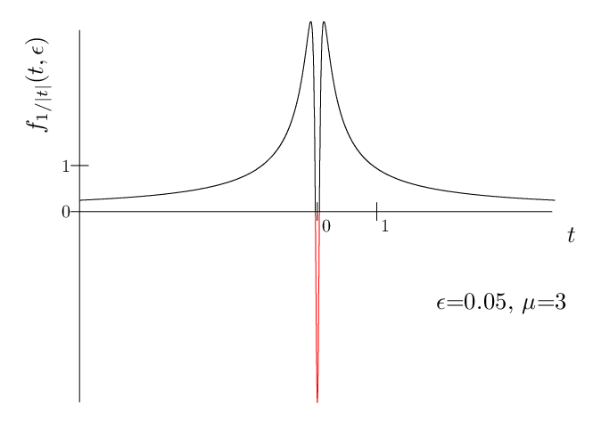
Refer to caption — Figure 1: Negative contribution around $t=0$ in regularised $f_{1/|t|}(t,\epsilon)$ (3)

For that reason, there appears to be a conflict between the demands of positivity for certain coefficients in the Hamiltonian arising if one pursues a geometrical interpretation, and negative contributions introduced by our “minimal subtraction” recipe. If one is to construct a geometrical resolution of dynamics on a singular space-time background, one generally needs to relax the specifications of the “minimal subtraction” approach, and permit modifications in the operator structure of the Hamiltonian, as well as its time dependence, in the vicinity of the singular region. One will then typically end up with a situation where a few different operator structures in the Hamiltonian essentially contribute to the transition to the singular region:

H(t)=\sum\limits_{i}f_{i}(t,\varepsilon)H_{i},

(6)

where $H_{i}$ are time-independent operators and $f_{i}$ are time-dependent number-valued functions. $\varepsilon$ is a regularization parameter, and the implication is that, as $\varepsilon$ is taken to 0, some of the $f_{i}$ ’s may develop isolated singularities at a certain value of $t$ , which we shall choose to be $t=0$ . It is the commutation properties of those different terms in the Hamiltonian that are responsible for divergence cancellation (rather than explicit negative contributions introduced through the “minimal subtraction” scheme of [13]).

In what follows, we shall review some relevant properties of quantum time-dependent Hamiltonians involving multiple operator structures, and proceed with applying this range of techniques to constructing singular limits of dynamics in a few different geometrical backgrounds related to the null-brane space-time. In section 2, we start by discussing the evolution properties for Hamiltonians of the form (6). In section 3, we examine as an example the null-brane, which is the geometric resolution (through a parameter $R$ , which plays the role of $\epsilon$ in this case) of the parabolic orbifold. We introduce a generalized null-brane metric depending on continuous parameters $(R,\alpha,\beta)$ . The propagation of a free scalar field on this space-time will be described by computing its mode functions, derived by solving the wave equation exactly using WKB methods. Then we discuss properties of the mode functions of a free scalar field in the singular limit $R\to 0$ . We shall find that the limit of the mode functions exists for certain discrete values of the parameters $\alpha$ and $\beta$ . We give a qualitative discussion of the results in subsection 3.3. In section 4, we introduce the light-like reflector plane, a simple yet curious space-time that can be used as a toy model for light-like space-time singularities. Section 5 contains our conclusions. Appendix A contains a discussion of the minimal subtraction prescription of [13] applied to the parabolic orbifold. In appendix B, we give some technical details related to focusing properties and Maslov phases.

2 Time-dependent Hamiltonians involving multiple operator structures

In preparation for our analysis of geometrical resolutions and their singular limits, we shall review the quantum dynamics described by Hamiltonians of the form (6). Our ultimate question will be whether the $\varepsilon\to 0$ limit of the evolution operator corresponding to (6) exists.

It is in general impossible to solve the Schrödinger equation corresponding to the Hamiltonian (6). The familiar symbolic solution for the evolution operator $U(t_{1},t_{2})$ involves the time-ordering symbol T:

U(t_{1},t_{2})={\mbox{T}}\left[-i\int\limits_{t_{1}}^{t_{2}}dt\,H(t)\right].

(7)

The above representation can be further transformed in an instructive way using a technique known as the Magnus expansion [14]. The operator $U$ belongs to the group of unitary operators on the Hilbert space, and the Magnus expansion can be thought of as an analog of the Baker-Campbell-Hausdorff formula for finite-dimensional Lie groups (the latter is discussed in many textbooks on group theory, for example, in [15]). The expansion can be symbolically written as:

\begin{array}[]{l}\displaystyle U(t_{1},t_{2})=\exp\left[-i\int\limits_{t_{1}}^{t_{2}}dt\,H(t)+\eta_{1}\int dt\,dt^{\prime}\,[H(t),H(t^{\prime})]\right.\\ \displaystyle\hskip 113.81102pt\left.+i\,\eta_{2}\int dt\,dt^{\prime}\,dt^{\prime\prime}\,[H(t),[H(t^{\prime}),H(t^{\prime\prime})]]+\cdots\right],\end{array}

(8)

with some numerical coefficients $\eta_{1}$ , $\eta_{2},\ldots$ (their values will not be important for us, and it appears they can only be derived recursively [14]). The key property of the above expression is that the higher order terms are entirely expressed through higher order nested commutators of $H(t)$ at different moments of time.

Even though, in a completely general setting, the Magnus expansion is hopelessly intractable, it displays the broad range of opportunities for divergence cancellation in a singular limit of the dynamics described by (6). Namely, for the case of (6), the Magnus expansion (8) will contain all kinds of combinations of the $f_{i}$ and their products, in such a way that, even if $f_{i}$ develop very strong singularities as $\varepsilon$ is taken to 0, the limit of $U(t_{1},t_{2})$ may still exist. For example, even if all $f_{i}$ are positive, cancellations may still occur on account of the commutation properties of $H_{i}$ .

Should such cancellations take place, one may think of the $\varepsilon\to 0$ limit of (6) as an operator-valued generalization of conventional distributions: just as ordinary distributions may contain singularities in a way that permits evaluating ordinary integrals, the Hamiltonian (6) will contain singularities in a way that permits evaluating the time-ordered exponential integral in (7). A systematic exploration of such generalized operator-valued “distributions” may be interesting to pursue, but lies outside of the scope of the present paper.

There is a special case when the above analysis can be taken significantly further. Namely, it may turn out that, for all moments of time, the operator $U$ of (7) belongs to a finite-dimensional subgroup of the unitary group of the Hilbert space. This situation has been described as a presence of a dynamical group (see [16, 17] and references therein). For the Hamiltonians of the form (6), there will exist a finite-dimensional dynamical group if the set of nested commutators of $H_{i}$ ’s closes on a finite-dimensional linear space of operators (which would serve as the Lie algebra of the dynamical group). Should that happen, one would be able to use the the closed resummed version of the Baker-Campbell-Hausdorff formula for finite-dimensional Lie groups (see, for example, [15]) to treat the Magnus expansion, or, alternatively, the Schrödinger equation can be reduced to a finite number of ordinary differential equations³³ 3 The analytic power of the dynamical group approach does not appear completely clear or fully explored. It certainly does apply to all linear quantum systems; however, in that case, the conventional WKB analysis would suffice. Beyond linear systems, the relevant finite-dimensional subalgebras of Hermitean operators may be difficult to construct and/or classify. Nevertheless, some non-trivial examples of dynamical groups for quantum-mechanical systems do exist (see, for example, [19]). describing the evolution on the finite-dimensional dynamical group manifold [16, 17, 18]. In practical terms, one can choose a particular low-dimensional faithful linear representation of the dynamical group furnished by matrices $M$ , and write down the Schrödinger equation in this representation:

i\frac{dM(t,t_{0})}{dt}=\varphi(H(t))M,\qquad M(t_{0},t_{0})=1,

(9)

where $\varphi$ is a homomorphism from Hilbert space operators onto the representation furnished by $M$ . (This is a finite-dimensional system of ordinary differential equations.) Given the solution for $M(t,t_{0})$ , one can reconstruct the original evolution operator as $\varphi^{-1}(M(t,t_{0}))$ .

While the specific examples of quantum dynamics discussed in this paper will be constructed using a somewhat unconventional application of WKB methods, the fact this “double-semiclassical” analysis is possible reflects an underlying dynamical group structure inherent to the systems we shall work with. After explicitly computing the mode functions encoding the dynamics, we shall investigate (in this greatly simplified setting) the existence of singular limits. It will then be possible to circumnavigate the formal complications introduced by the non-commuting structures in (6), and examine the limiting case of evolution on a singular space-time background.

3 Generalized null-brane space-times and singular limits

In this section, we study quantum dynamics of a free scalar field propagating on the parabolic orbifold and some geometrical resolutions thereof, including the null-brane.

3.1 The null-brane geometry, the parabolic orbifold and generalizations

The null-brane spacetime, originally introduced in [4], was studied in the context of perturbative string theory in [8, 23, 24]; a matrix theory description was provided in [3].

Consider Minkowski space-time in light-cone coordinates $ds^{2}=-2dx^{+}dx^{-}+dx^{2}+dz^{2}$ . The null-brane is obtained by identifying

\displaystyle\begin{bmatrix}x^{+}\\ x\\ x^{-}\\ \end{bmatrix}\sim\mathrm{exp}(2\pi n\mathcal{J})\begin{bmatrix}x^{+}\\ x\\ x^{-}\\ \end{bmatrix}\,,\hskip 28.45274ptz\sim z+2\pi nR\,,\hskip 28.45274ptn\in\mathbb{Z}\,,\hskip 28.45274pt\mathcal{J}=\begin{bmatrix}0&0&0\\ 1&0&0\\ 0&1&0\\ \end{bmatrix}.

(10)

In the $R\rightarrow 0$ limit the null-brane reduces to the parabolic orbifold [5, 7] times the line labeled by $z$ . In this sense, the null-brane is a geometrical regularization of the parabolic orbifold. In Rosen coordinates, the metric on the parabolic orbifold is given by

ds^{2}=-2dy^{+}dy^{-}+(y^{+})^{2}dy^{2}.

(11)

In [8], the null-brane geometry was discussed in two coordinate systems,

	$\displaystyle ds^{2}$	$\displaystyle=$	$\displaystyle-2dy^{+}dy^{-}+du^{2}+(R^{2}+(y^{+})^{2})dy^{2}+2Rdydu;$		(12)
	$\displaystyle ds^{2}$	$\displaystyle=$	$\displaystyle-2d\tilde{x}^{+}d\tilde{x}^{-}+d\tilde{x}^{2}+(R^{2}+\tilde{x}^{2})d\theta^{2}+2(\tilde{x}^{+}d\tilde{x}-\tilde{x}d\tilde{x}^{+})d\theta,$		(13)

related to Minkowski coordinates by

	$\displaystyle x^{+}=y^{+},\;x=yy^{+},\;x^{-}=y^{-}+\frac{1}{2}y^{+}y^{2},\;u=z-Ry;$		(14)
	$\displaystyle x^{+}=\tilde{x}^{+},\;x=\tilde{x}+\theta\tilde{x}^{+},\;x^{-}=\tilde{x}^{-}+\theta\tilde{x}+\frac{1}{2}\theta^{2}\tilde{x}^{+},\;\theta=\frac{z}{R}.$		(15)

Unfortunately, neither coordinate system is fully satisfactory for studying the $R\to 0$ limit of dynamics on the null-brane.⁴⁴ 4 Following the discussion in the previous section, with $R$ playing the role of $\epsilon$ , we would like to phrase the dynamics in terms of a Hamiltonian that has the structure $H=\sum_{i}f_{i}(t,R)H_{i}$ in which $f_{i}(t,R)$ is regular in $t$ for $R\neq 0$ and regular away from $t=0$ for $R=0$ . The terms that appear in the Hamiltonian can be easily deduced from the inverse metric. On the one hand, the $y\text{-coordinates}$ are not globally defined since they are singular at $y^{+}=0$ for any $R$ . On the other hand, the $\tilde{x}\text{-coordinates}$ , which are nonsingular for $R\neq 0$ , do not have an $R\to 0$ limit even away from the parabolic orbifold singularity, as the determinant of the metric is $-R^{2}$ everywhere.

Therefore, we now introduce new coordinates that interpolate between the $\tilde{x}\text{-coordinates}$ (for small $\tilde{x}^{+}$ ) and the $y\text{-coordinates}$ (for large $y^{+}$ ):

$\displaystyle X^{+}$	$\displaystyle=$	$\displaystyle\tilde{x}^{+}=y^{+};$	(16)
$\displaystyle X^{-}$	$\displaystyle=$	$\displaystyle\tilde{x}^{-}-\frac{1}{2}\frac{\tilde{x}}{\tilde{x}^{+}}\left(1-\frac{R^{4}}{\left(R^{2}+(\tilde{x}^{+})^{2}\right)^{2}}\right)=y^{-}+\frac{R^{2}}{2}\frac{y^{+}u^{2}}{\left(R^{2}+(y^{+})^{2}\right)^{2}};$
$\displaystyle X$	$\displaystyle=$	$\displaystyle-\frac{R\tilde{x}}{\sqrt{R^{2}+(\tilde{x}^{+})^{2}}}=\frac{y^{+}u}{\sqrt{R^{2}+(y^{+})^{2}}};$
$\displaystyle\Theta$	$\displaystyle=$	$\displaystyle\theta+\frac{\tilde{x}}{\tilde{x}^{+}}\left(1-\frac{R^{2}}{R^{2}+(\tilde{x}^{+})^{2}}\right)=y+\frac{Ru}{R^{2}+(y^{+})^{2}}.$

In this coordinate system, the metric has determinant $-(R^{2}+(X^{+})^{2})$ .

The metric of the null-brane space-time, written in our new coordinates, can be naturally generalized to a two-parameter family of metrics, which we will call generalized null-brane. The family is labeled by parameters $\alpha$ and $\beta$ , the original null-brane corresponding to $\alpha=3,\beta=2$ :

ds^{2}=\frac{R^{2}X^{2}\left(\beta^{2}-\alpha\right)}{\left(R^{2}+(X^{+})^{2}\right)^{2}}\left(dX^{+}\right)^{2}\,-2dX^{+}dX^{-}+\frac{2\beta RX}{\sqrt{R^{2}+(X^{+})^{2}}}dX^{+}d\Theta+\left(R^{2}+(X^{+})^{2}\right)d\Theta^{2}+dX^{2}.

(17)

3.2 Free scalar field on the generalized null-brane

3.2.1 General dynamical preliminaries

We consider a free scalar field on the generalized null-brane metric. After Fourier transforming with respect to $X^{-}$ and $\Theta$ ,

\phi(X^{+},X^{-},X,\Theta)=\frac{1}{2\pi}\sum_{k_{\Theta}}\int dk_{-}\phi_{k_{-},k_{\Theta}}\mathrm{exp}\left(ik_{-}X^{-}+ik_{\Theta}\Theta\right),

(18)

and suppressing the indices $k_{-}$ and $k_{\Theta}$ , the action reads

	$\displaystyle S$	$\displaystyle=$	$\displaystyle\sum_{k_{\Theta}}\int\mathrm{d}X^{+}\,\mathrm{d}k_{-}\,\mathrm{d}X\,\,\,\sqrt{R^{2}+(X^{+})^{2}}\Biggl[\frac{ik_{-}}{2}\bigl(\phi\partial_{X^{+}}\phi^{}-\phi^{}\partial_{X^{+}}\phi\bigr)-\frac{\partial_{X}\phi\partial_{X}\phi^{*}}{2}$		(19)
			$\displaystyle\ \ \ \ \ \ \ \ \ -\biggl(\frac{m^{2}}{2}+\frac{k_{\Theta}^{2}}{2(R^{2}+(X^{+})^{2})}+\frac{\alpha X^{2}R^{2}k_{-}^{2}}{2(R^{2}+(X^{+})^{2})^{2}}+\frac{k_{\Theta}k_{-}\beta XR}{(R^{2}+(X^{+})^{2})^{3/2}}\biggr)\phi\phi^{*}\Biggr].$		(19)

Denoting $\partial_{X^{+}}\phi$ as $\dot{\phi}$ , the wave equation reads

	$\displaystyle-i\dot{\phi}$	$\displaystyle=$	$\displaystyle\frac{iX^{+}}{2\left(R^{2}+(X^{+})^{2}\right)}\phi-\frac{\partial^{2}_{X}\phi}{2k_{-}}+\frac{\beta XRk_{\Theta}}{\bigl(R^{2}+(X^{+})^{2}\bigr)^{3/2}}\phi$		(20)
			$\displaystyle\hskip 11.38109pt+\frac{k_{\Theta}^{2}}{2k_{-}\left(R^{2}+(X^{+})^{2}\right)}\phi+\frac{\alpha}{2}\frac{X^{2}R^{2}k_{-}}{\bigl(R^{2}+(X^{+})^{2}\bigr)^{2}}\phi+\frac{m^{2}}{2k_{-}}\phi.$		(20)

As the Lagrangian is first order in time derivatives, we have to deal, in principle, with constraints when deriving the corresponding Hamiltonian. One can take a shortcut interpreting $\phi$ as a canonical coordinate and $\pi\equiv ik_{-}\sqrt{R^{2}+(X^{+})^{2}}\phi^{*}$ as its conjugate momentum. The Hamiltonian reads

	$\displaystyle H$	$\displaystyle=$	$\displaystyle\sum_{k_{\Theta}}\sum_{k_{-}\not=0}\int\,\mathrm{d}X\,\pi\Biggl[\frac{X^{+}}{2\left(R^{2}+(X^{+})^{2}\right)}-\frac{im^{2}}{2k_{-}}+\frac{i}{2k_{-}}\partial^{2}_{X}-\frac{i\beta XRk_{\Theta}}{\bigl(R^{2}+(X^{+})^{2}\bigr)^{3/2}}$		(21)
			$\displaystyle\ \ \ \ \ \ \ \ \ \ \ \ \ \ \ \ \ -\frac{i}{2k_{-}}\frac{k_{\Theta}^{2}}{R^{2}+(X^{+})^{2}}-\frac{i\alpha}{2}\frac{X^{2}R^{2}k_{-}}{\bigl(R^{2}+(X^{+})^{2}\bigr)^{2}}\Biggr]\phi.$		(21)

It is manifestly of the form $H=\sum_{i}f_{i}(t,R)H_{i}$ , in other words, it belongs to the class of Hamiltonians we single out in section 2.

We now show that the Hamiltonian (21) leads to a finite-dimensional dynamical group structure of the type discussed in section 2. The canonical variables $\pi(X,t)$ and $\phi(X,t)$ appear in four combinations $\int\pi\,\partial_{X}^{2}\phi,\;\int\pi\phi,\;\int\pi X\phi\;\text{and}\;\int\pi X^{2}\phi$ . The commutation relations for such operators are given by

\left[\int\pi\,\hat{A}(X)\,\phi\,dX\,,\;\int\pi\,\hat{B}(X)\,\phi\,dX\right]=\int\pi[\hat{A},\hat{B}]\phi\,dX,

(22)

reducing the commutator algebra to that of $\{\partial^{2}_{X},\,1,\,X,\,X^{2}\}$ , which closes after the addition of $\{X\partial_{X},\,\partial_{X}\}$ . Equivalently, one can form the standard (single degree of freedom) creation and annihilation operators $a$ and $a^{\dagger}$ out of $X$ and $\partial_{X}$ to conclude that the Lie algebra of the dynamical group is spanned by $n=a^{\dagger}a+1/2,a^{\dagger 2},a^{2},a^{\dagger},a$ and $I$ . Given the inclusion of powers of the creation operator up to $a^{\dagger 2}$ , it is not surprising that the corresponding algebra has become known as the two-photon algebra, or $h_{6}$ , and has been featured in discussions of quantum optics, and squeezed states in particular (see, for example [16]). A complete formal analysis of quantum dynamics on the two-photon group has been given in [18].

Following the general picture presented in section 2, we could use the two-photon group considerations of [18] to reduce the question of free scalar field dynamics on the generalized null-brane to ordinary differential equations. In our present setting, however, one can perform these operations in a considerably more familiar guise. Namely, since the free scalar field is linear, solving for its quantum dynamics amounts to constructing a complete set of solutions to the classical wave equation. Furthermore, the classical wave equation turns out to be equivalent to the Schrödinger equation for a linear auxiliary one-dimensional quantum system. Because the auxiliary system is linear, its Schrödinger equation (i.e., the wave equation of the original scalar field) can be solved exactly by WKB methods. The latter effectively reduce the problem to ordinary differential equations (the classical equations of motion of the auxiliary linear system). Thus, one attains the same level of simplification as one would through performing the analysis of [18]. One can refer to the above procedure as “double-semiclassical” analysis (there is an (exact) WKB procedure leading from a free quantum scalar field to the wave equation for the mode functions, and an (exact) WKB procedure leading from the wave equation for the mode functions to a one-dimensional auxiliary classical system). Note that both the “double-semiclassical” approach and the general dynamical group approach of [18] (which are essentially one and the same thing) are made possible by the fact that the metric of the generalized null-brane is a quadratic polynomial in the $X$ -variable.

For linear quantum systems, it is most common to work in the Heisenberg picture, instead of (equivalently) deriving WKB wave functions in the Schrödinger picture. One obtains the solution for the Heisenberg field operator as an expansion in terms of a complete set of mode functions $u_{y}(X,X^{+})$ (with $y$ being a generic basis label) satisfying the classical equations of motion:

\phi_{k_{-},k_{\Theta}}=\int\mathrm{d}y\;u_{y}(X,X^{+})a(y).

(23)

The corresponding conjugate momentum is

\pi_{k_{-},k_{\Theta}}=ik_{-}\sqrt{R^{2}+\left(X^{+}\right)^{2}}\int\mathrm{d}y\;u^{*}_{y}(X,X^{+})a^{\dagger}(y).

(24)

If one demands the standard commutation relations for the creation-annihilation operators $a^{\dagger}$ and $a$ , the canonical commutation relation between $\pi$ and $\phi$ determine the normalisation of the mode functions (this is the analog for first order systems of the Klein-Gordon norm):

\delta(X-\tilde{X})=k_{-}\sqrt{R^{2}+\left(X^{+}\right)^{2}}\int\mathrm{d}y\;u_{y}^{*}(X,X^{+})u_{y}(\tilde{X},X^{+}).

(25)

3.2.2 “Double-semiclassical” solution of the wave equation

Denoting $X^{+}$ by $t$ , (20) takes the form of an auxiliary Schrödinger equation with Hamiltonian

\mathcal{H}=\frac{it}{2\left(R^{2}+t^{2}\right)}+\frac{P^{2}}{2k_{-}}+\frac{\beta XRk_{\Theta}}{\bigl(R^{2}+t^{2}\bigr)^{3/2}}+\frac{k_{\Theta}^{2}}{2k_{-}\left(R^{2}+t^{2}\right)}+\frac{\alpha}{2}\frac{X^{2}R^{2}k_{-}}{\bigl(R^{2}+t^{2}\bigr)^{2}}+\frac{m^{2}}{2k_{-}}

(26)

(up to a sign difference in the left hand side of (20)). As the corresponding Hamiltonian (26) is quadratic in $X$ , (20) can be solved exactly by WKB methods. The starting point is the observation that the ansatz

\phi(X_{1},t_{1}|X_{2},t_{2})={\cal A}(t_{1},t_{2})\mathrm{exp}\left(-iS_{cl}\left[X_{1},t_{1}|X_{2},t_{2}\right]\right)

(27)

solves (20) (with $t_{2}\to t$ ) if

	$\displaystyle S_{cl}=\int_{t_{1}}^{t_{2}}\,\mathrm{d}t\,\left(P\dot{X}-\mathcal{H}\right){\Big\|_{X=X_{cl}(X_{1},t_{1}\|X_{2},t_{2})}};$		(28)
	$\displaystyle-2k_{-}\,\frac{\partial{\cal A}(t_{1},t)}{\partial t}={\cal A}(t_{1},t)\,\frac{\partial^{2}S_{cl}\left[X_{1},t_{1}\|X,t\right]}{\partial X^{2}}.$		(29)

Here, $S_{cl}$ is the classical action with boundary conditions $X(t_{1})=X_{1},\ X(t_{2})=X_{2}$ . More general solutions to (20) are obtained by integrating (27) over $X_{1}$ , weighted by an arbitrary smooth wavepacket.

A subtlety arises in this ansatz when the dynamical evolution reaches a focal point $t_{2}=t^{*}$ , where the classical action diverges, unless a certain relation between $X_{1}$ (“the source”) and $X_{2}$ (“the image”) is met. At such focal points, the differential equation for ${\cal A}(t_{1},t_{2})$ becomes singular. In that case, one solves the WKB equations away from $t^{*}$ and connects the solution by a phase jump at the focal point. The phase jump should be chosen such that convolutions of (27) with a smooth wavepacket are continuous across the focal point. The general guidelines for this procedure are best familiar in the context of caustic submanifolds in geometrical optics (see, for example, [20, 21]) and the above-mentioned correction pre-factors have become known as the Maslov phases. We shall give some further details in appendix B.

In order to compute the classical action, we first consider the classical equation of motion:


		$\displaystyle\ddot{X}+\alpha\frac{R^{2}}{\bigl(R^{2}+t^{2}\bigr)^{2}}X=-\frac{\beta k_{\Theta}}{k_{-}}\frac{R}{\bigl(R^{2}+t^{2}\bigr)^{3/2}},$		(30a)
		$\displaystyle X(t_{1})=X_{1},\qquad X(t_{2})=X_{2}.$		(30b)

This equation is actually exactly solvable, and it has become known as the equation for “bending of a double-walled compressed bar with a parabolic cross-section” [22]. It can be reduced to a driven harmonic oscillator with constant frequency via substitution $X=\sqrt{R^{2}+t^{2}}\chi(\eta(t))$ , taking $\eta=\mathrm{arctan}(t/R)$ :

\frac{d^{2}\chi}{d\eta^{2}}+\left(1+\alpha\right)\,\chi=-\frac{\beta k_{\Theta}}{Rk_{-}}.

(31)

In order to give a transparent derivation of the solution to (30) and the corresponding value of the classical action, we first consider the two independent solutions to the homogeneous version of (30a):


	$\displaystyle f(t)=\sqrt{R^{2}+t^{2}}\;\mathrm{sin}\left(\sqrt{1+\alpha}\,\mathrm{arctan}\frac{t}{R}\right),$		(32a)
	$\displaystyle h(t)=\sqrt{R^{2}+t^{2}}\;\mathrm{cos}\left(\sqrt{1+\alpha}\,\mathrm{arctan}\frac{t}{R}\right).$		(32b)

A useful object to consider is the Dirichlet Green function of the operator $\partial^{2}_{t}+\alpha R^{2}/\bigl(R^{2}+t^{2}\bigr)^{2}$ :

G(t,t^{\prime}|t_{1},t_{2})=\frac{\left(f_{1}h(t_{<})-h_{1}f(t_{<})\right)\left(f_{2}h(t_{>})-h_{2}f(t_{>})\right)}{W[f,h](f_{1}h_{2}-h_{1}f_{2})},

(33)

satisfying

\left(\partial^{2}_{t}+\frac{\alpha R^{2}}{\bigl(R^{2}+t^{2}\bigr)^{2}}\right)G(t,t^{\prime}|t_{1},t_{2})=\delta(t-t^{\prime}),\qquad G(t_{1},t^{\prime}|t_{1},t_{2})=0,\qquad G(t_{2},t^{\prime}|t_{1},t_{2})=0

(34)

with $W[f,h]=f\dot{h}-h\dot{f}$ being the Wronskian of $f(t)$ and $h(t)$ (independent of $t$ ), $t_{2}>t_{1}$ , $t_{<}=\mathrm{min}(t,t^{\prime})$ , $t_{>}=\mathrm{max}(t,t^{\prime})$ and $f_{1}=f(t_{1})$ , $h_{1}=h(t_{1})$ , etc.

With the Green function given by (33), and $b(t)$ denoting the right hand side of equation (30a), one can write down the solution to (30) as

\begin{array}[]{l}\displaystyle X_{cl}(t|X_{1},t_{1};X_{2},t_{2})=-X_{1}\partial_{t^{\prime}}G(t,t^{\prime}|t_{1},t_{2})\Big|_{t^{\prime}=t_{1}}+X_{2}\partial_{t^{\prime}}G(t,t^{\prime}|t_{1},t_{2})\Big|_{t^{\prime}=t_{2}}\\ \displaystyle\hskip 199.16928pt+\int\limits_{t_{1}}^{t_{2}}dt^{\prime}\,G(t,t^{\prime}|t_{1},t_{2})b(t^{\prime})\end{array}

(35)

Given the above formulas, the classical action can be written in a relatively general form that will turn out to be useful later:


		$\displaystyle S_{cl}=-\frac{k_{-}}{2}\left[\frac{h_{2}\dot{f}_{1}-f_{2}\dot{h}_{1}}{f_{1}h_{2}-h_{1}f_{2}}\right]X^{2}_{1}+\frac{k_{-}}{2}\left[\frac{f_{1}\dot{h}_{2}-h_{1}\dot{f}_{2}}{f_{1}h_{2}-h_{1}f_{2}}\right]X^{2}_{2}-k_{-}\left[\frac{W[f,h]}{f_{1}h_{2}-h_{1}f_{2}}\right]X_{1}X_{2}$		(36a)
		$\displaystyle-k_{-}\int_{t_{1}}^{t_{2}}\mathrm{d}t\,\,b(t)\,\left(\frac{h_{2}f(t)-f_{2}h(t)}{f_{1}h_{2}-f_{2}h_{1}}\right)X_{1}-k_{-}\int_{t_{1}}^{t_{2}}\mathrm{d}t\,\,b(t)\,\left(\frac{f_{1}h(t)-h_{1}f(t)}{f_{1}h_{2}-f_{2}h_{1}}\right)X_{2}$		(36b)
		$\displaystyle+k_{-}\int_{t_{1}}^{t_{2}}\mathrm{d}t^{\prime}\int_{t_{1}}^{t^{\prime}}\mathrm{d}t\,\,b(t)\frac{\bigl(f_{1}h(t)-h_{1}f(t)\bigr)\bigl(f_{2}h(t^{\prime})-h_{2}f(t^{\prime})\bigr)}{W[f,h](f_{1}h_{2}-h_{1}f_{2})}b(t^{\prime})$		(36c)
		$\displaystyle-\frac{m^{2}}{2k_{-}}(t_{2}-t_{1})-\frac{i}{2}\ln\frac{\sqrt{R^{2}+{t_{2}}^{2}}}{\sqrt{R^{2}+{t_{1}}^{2}}}$		(36d)

Of course, one can also solve the equations of motion (30) explicitly:


$\displaystyle\displaystyle X=X_{1}\frac{\sqrt{R^{2}+t^{2}}}{\sqrt{R^{2}+t_{1}^{2}}}\frac{\mathrm{sin}2\Delta_{t2}}{\,\mathrm{sin}2\Delta_{12}\,}$	$\displaystyle+X_{2}\frac{\sqrt{R^{2}+t^{2}}}{\sqrt{R^{2}+t_{2}^{2}}}\frac{\mathrm{sin}2\Delta_{1t}}{\,\mathrm{sin}2\Delta_{12}\,}$
	$\displaystyle-\frac{\beta k_{\Theta}\sqrt{R^{2}+t^{2}}}{Rk_{-}(1+\alpha)}\biggl[1-\frac{\mathrm{sin}2\Delta_{t2}}{\,\mathrm{sin}2\Delta_{12}\,}-\frac{\mathrm{sin}2\Delta_{1t}}{\,\mathrm{sin}2\Delta_{12}\,}\biggr]$	(37a)
$\displaystyle\Delta_{12}=\frac{\sqrt{1+\alpha}}{2}$	$\displaystyle\left(\mathrm{arctan}\frac{t_{2}}{R}-\mathrm{arctan}\frac{t_{1}}{R}\right)$	(37b)
$\displaystyle\Delta_{t2}=\frac{\sqrt{1+\alpha}}{2}$	$\displaystyle\left(\mathrm{arctan}\frac{t_{2}}{R}-\mathrm{arctan}\frac{t}{R}\right)$	(37c)
$\displaystyle\Delta_{1t}=\frac{\sqrt{1+\alpha}}{2}$	$\displaystyle\left(\mathrm{arctan}\frac{t}{R}-\mathrm{arctan}\frac{t_{1}}{R}\right)$	(37d)

The classical action can now be evaluated either by brute force using the explicit classical solution (37), or, with less work, from (36):


$\displaystyle\displaystyle S_{cl}[X_{1},t_{1}\|X_{2},t_{2}]=$	$\displaystyle-k_{-}\,\Bigl[\frac{t_{1}}{2\left(R^{2}+t_{1}^{2}\right)}-\frac{R\,\sqrt{1+\alpha}}{2\left(R^{2}+t_{1}^{2}\right)}\,\mathrm{cot}2\Delta_{12}\,\Bigr]X^{2}_{1}$	(38a)
	$\displaystyle+k_{-}\,\Bigl[\frac{t_{2}}{2\left(R^{2}+t_{2}^{2}\right)}+\frac{R\,\sqrt{1+\alpha}}{2\left(R^{2}+t_{2}^{2}\right)}\,\mathrm{cot}2\Delta_{12}\,\Bigr]X^{2}_{2}\vskip 8.53581pt$	(38b)
	$\displaystyle-\Bigl[\frac{k_{-}\,\sqrt{1+\alpha}\,R}{\sqrt{R^{2}+t_{1}^{2}}\sqrt{R^{2}+t_{2}^{2}}\,\,\mathrm{sin}2\Delta_{12}\,}\Bigr]X_{1}X_{2}$	(38c)
	$\displaystyle-\Bigl[\frac{\beta\,k_{\Theta}}{\sqrt{1+\alpha}\sqrt{R^{2}+t_{1}^{2}}}\mathrm{tan}\Delta_{12}\Bigr]X_{1}$	(38d)
	$\displaystyle-\Bigl[\frac{\beta\,k_{\Theta}}{\sqrt{1+\alpha}\sqrt{R^{2}+t_{2}^{2}}}\mathrm{tan}\Delta_{12}\Bigr]X_{2}$	(38e)
	$\displaystyle-\frac{\beta^{2}\,k_{\Theta}^{2}}{k_{-}\left(1+\alpha\right)^{3/2}\,R}\Bigl(\mathrm{tan}\Delta_{12}\,-\Delta_{12}\Bigr)$	(38f)
	$\displaystyle-\frac{m^{2}}{2k_{-}}(t_{2}-t_{1})-\frac{i}{2}\ln\frac{\sqrt{R^{2}+{t_{2}}^{2}}}{\sqrt{R^{2}+{t_{1}}^{2}}}-\frac{k_{\Theta}^{2}\Delta_{12}}{k_{-}\,R\,\sqrt{1+\alpha}}.$	(38g)

Next we consider the “quantum-mechanical” prefactor (40). With the expression for $S_{cl}$ given by (36), equation (29) becomes:

\frac{\partial{\cal A}(t_{1},t)}{\partial t}=-\frac{1}{2}\frac{f_{1}\dot{h}-h_{1}\dot{f}}{f_{1}h-h_{1}f}\,{\cal A}(t_{1},t).

(39)

This leads to the solution

{\cal A}(t_{1},t_{2})=\mathcal{N}\left(R^{2}+t_{1}^{2}\right)^{-1/4}\left(R^{2}+t_{2}^{2}\right)^{-1/4}\,\left|\,\mathrm{sin}2\Delta_{12}\right|^{-1/2}\phi_{M},

(40)

which contains the Maslov phase $\phi_{M}$ and a constant normalization factor $\mathcal{N}$ . The Maslov phase is piecewise constant away from the focal points (the positions of focal point for $t_{2}$ are functions of $t_{1}$ ). Its value is worked out in appendix B.

We can now fix the normalization of ${\cal A}(t_{1},t_{2})$ by imposing (25):

{\cal N}=\sqrt{\frac{R\sqrt{1+\alpha}}{2\pi\sqrt{R^{2}+t_{1}^{2}}}}

(41)

3.2.3 The $R\to 0$ limit

Now that we have constructed the “propagator” $\phi(X_{1},t_{1}|X_{2},t_{2})$ , which provides a basis of mode functions labelled by $X_{1}$ , we can investigate its $R\to 0$ limit, which will only exist for special values of $\alpha$ and $\beta$ .

The first non-trivial condition for the existence of an $R\to 0$ limit comes from the prefactor ${\cal A}(t_{1},t_{2})$ . This will vanish identically for $t_{1}<0$ , $t_{2}>0$ as $R$ is sent to 0 (which would make the field operator vanish identically and manifestly destroy unitarity), unless

\alpha=N^{2}-1,

(42)

with an integer $N$ , on account of the structure $\sqrt{R/\mathrm{sin}2\Delta_{12}}$ in (40) combined with (41).

This behavior of the prefactor ${\cal A}(t_{1},t_{2})$ can be naturally understood by inspecting the classical homogeneous solutions (32). For generic values of $\alpha$ and $\beta$ , in the $R\to 0$ limit, those behave as $f(t)\rightarrow t$ and $h(t)\rightarrow|t|$ . Since these two functions are not linearly independent on the negative real axis, one will not be able to specify arbitrary initial conditions $(X_{1}$ , $V_{1})$ for the classical solution at $t_{1}<0$ . Should one try to do so, in the $R\to 0$ limit, the classical trajectory will be kicked away to infinity for all $t>0$ . Correspondingly, all quantum wavepackets will be kicked away to infinity, and the wave function will vanish at all finite values of $X$ for $t>0$ , as manifested by the behavior of the prefactor ${\cal A}(t_{1},t_{2})$ . This problem is avoided, however, for special values of $\alpha$ : if $\alpha=(2N)^{2}-1$ (with an integer $N$ ), the $R\to 0$ limit of the two solutions is $f(t)\to\mathrm{sign}(t)$ and $h(t)\rightarrow|t|$ ; if $\alpha=(2N+1)^{2}-1$ , it is $f(t)\rightarrow t$ and $h(t)\to 1$ .

A further condition on $\alpha$ and $\beta$ arises from considering the $R\to 0$ limit of the classical action $S_{cl}[X_{1},t_{1}|X_{2},t_{2}]$ . The problematic terms in the action (38) are those with coefficients containing $k_{\Theta}^{2}$ , namely:

-\frac{\beta^{2}\,k_{\Theta}^{2}}{k_{-}(1+\alpha)^{3/2}\,R}\Bigl(\mathrm{tan}\Delta_{12}-\Delta_{12}\Bigr)-\frac{k_{\Theta}^{2}\Delta_{12}}{k_{-}\,R\,\sqrt{1+\alpha}}.

(43)

In order to cancel the divergences, we find the following equation for $\beta$ :

\beta^{2}=\frac{1+\alpha}{1-\dfrac{\mathrm{tan}\left(\pi\sqrt{1+\alpha}/2\right)}{\pi\sqrt{1+\alpha}/2}}.

(44)

If $\alpha=(2N+1)^{2}-1$ , this condition would make us naïvely conclude that $\beta=0$ . However, a direct inspection of (43) reveals that it wouldn’t make the divergence cancel. The only other option remaining is

\alpha=(2N)^{2}-1,\qquad\beta=2N

(45)

( $\beta=-2N$ corresponds to the same space written in different coordinates). These are the conditions for existence of an $R\to 0$ limit for a free scalar field dynamics on the generalized null-brane. As one would expect, the values $\alpha=3$ and $\beta=2$ corresponding to the original null-brane do meet these conditions (for $N=1$ ).

3.2.4 Mode functions in momentum basis

To facilitate comparison with earlier work, we shall now derive momentum basis mode functions using the position basis mode functions $\phi\left(X_{1},t_{1}|X_{2},t_{2}\right)$ of section 3.2.2. The existence of an $R\rightarrow 0$ limit will not be affected by such conversion. To obtain the momentum basis mode functions, we take a Fourier transform (with respect to $X_{1}$ ) of the “propagator” $\phi\left(X_{1},t_{1}|X_{2},t_{2}\right)$ to convert it to an incoming plane wave basis, cancel the “free evolution” by multiplying with $\mathrm{exp}\left[i\left(m^{2}+p^{2}\right)t_{1}/(2k_{-})\right]$ (we are simply using the freedom we have in defining the basis of mode functions), and take the $t_{1}\rightarrow-\infty$ limit (which refers our momentum labels to incoming waves in the infinite past). We shall also omit time-independent overall phase factors. Finally, we shall take the limit $t_{1}\rightarrow-\infty$ :

V_{k_{-},k_{\Theta},p,m}=\lim\limits_{t_{1}\rightarrow-\infty}\int_{-\infty}^{\infty}\,\mathrm{d}X_{1}\,{\cal A}(t_{1},t_{2})\,\mathrm{exp}\left(-iS_{cl}\right)\,\mathrm{exp}\left(ipX_{1}\right)\mathrm{exp}\left(\frac{i\left(m^{2}+p^{2}\right)t_{1}}{2k_{-}}\right)

(46)

To be consistent with our notation in the beginning of this section, we shall now switch back to writing $X^{+}$ instead of $t$ for all space-time quantities. We finally obtain the mode functions

\begin{array}[]{l}\displaystyle V_{k_{-},k_{\Theta},p,m}=\sqrt{\frac{2RN}{|k_{-}|\left(R^{2}+(X^{+})^{2}\right)|\,\mathrm{sin}2\Delta\,|}}\,\phi_{M}\\ \displaystyle\hskip 28.45274pt\times\mathrm{exp}\Bigl[\frac{-ik_{-}\,X^{2}}{2\left(R^{2}+(X^{+})^{2}\right)}\left(2NR\,\mathrm{cot}2\Delta\,+X^{+}\right)+\frac{i\,X}{\sqrt{R^{2}+\left(X^{+}\right)^{2}}}\left(k_{\Theta}\mathrm{tan}\Delta+\frac{2RNp}{\,\mathrm{sin}2\Delta\,}\right)\\ \displaystyle\hskip 42.67912pt+\frac{ipk_{\Theta}}{k_{-}}\mathrm{tan}\Delta-\frac{ip^{2}RN}{k_{-}}\,\mathrm{cot}2\Delta\,+\frac{ik_{\Theta}^{2}}{2k_{-}NR}\mathrm{tan}\Delta+\frac{im^{2}X^{+}}{2k_{-}}+ik_{-}X^{-}+ik_{\Theta},\Theta\Bigr]\end{array}

(47)

where $\Delta=N\mathrm{arctan}(X^{+}/R)+\pi N/2$ .

For $R\rightarrow 0$ we obtain:

	$\displaystyle\displaystyle V_{k_{-},k_{\Theta},p,m}=$	$\displaystyle\frac{1}{\sqrt{\|k_{-}X^{+}\|}}\mathrm{exp}\left(\frac{i\pi}{2}\mathrm{sign}(k_{-})(2N-1)\theta(X^{+})\right)\vskip 5.69054pt$
		$\displaystyle\times\mathrm{exp}\Bigl[-ipX\,\mathrm{sign}(X^{+})+\frac{ip^{2}X^{+}}{k_{-}}-\frac{ik_{\Theta}^{2}}{2k_{-}X^{+}}+\frac{im^{2}X^{+}}{2k_{-}}+ik_{-}X^{-}+ik_{\Theta}\Theta\Bigr],$		(48)

where $\theta(t)$ denotes the Heaviside step function.

In order to compare our mode functions (47) with those derived in [8], we write out the mode functions for $N=1$ explicitly:

\begin{array}[]{l}\displaystyle V_{k_{-},k_{\Theta},p,m}^{(N=1)}=\frac{1}{\sqrt{|k_{-}X^{+}|}}\phi_{M}\mathrm{exp}\Bigl[\frac{-ik_{-}\,R^{2}X^{2}}{2X^{+}\left(R^{2}+(X^{+})^{2}\right)}-\frac{iX}{\sqrt{R^{2}+(X^{+})^{2}}}\left(k_{\Theta}\frac{R}{X^{+}}+p\frac{R^{2}+(X^{+})^{2}}{X^{+}}\right)\\ \displaystyle\hskip 28.45274pt-\frac{ipk_{\Theta}R}{k_{-}X^{+}}-\frac{ip^{2}}{k_{-}}\left(\frac{R^{2}-(X^{+})^{2}}{2X^{+}}\right)-\frac{ik_{\Theta}^{2}}{2k_{-}X^{+}}+\frac{im^{2}X^{+}}{2k_{-}}+ik_{-}X^{-}+ik_{\Theta}\Theta\Bigr].\end{array}

(49)

The general expression for the Maslov phase $\phi_{M}$ is given in appendix B. For $N=1$ , there is only one focal point at $X^{+}=0$ , and the Maslov phase becomes:

\phi_{M}=\mathrm{exp}\left(\frac{i\pi}{2}\mathrm{sign}(k_{-})\,\theta(X^{+})\right).

(50)

Written in our interpolating coordinates from (16), the mode functions of [8] can be re-expressed as

\begin{array}[]{l}\displaystyle\frac{1}{\sqrt{iX^{+}}}\mathrm{exp}\Bigl[\frac{ip^{+}R^{2}X^{2}}{2X^{+}\left(R^{2}+(X^{+})^{2}\right)}-\frac{i\,X}{\sqrt{R^{2}+(X^{+})^{2}}}\left(J\frac{R^{2}+(X^{+})^{2}}{RX^{+}}-n\frac{X^{+}}{R}\right)\\ \displaystyle\hskip 71.13188pt-\frac{iX^{+}}{2p^{+}}\left(\frac{n-J}{R}\right)^{2}+\frac{iJ^{2}}{2p^{+}X^{+}}-\frac{im^{2}X^{+}}{2p^{+}}-ip^{+}X^{-}+in\Theta\Bigr],\end{array}

(51)

with $J$ , $n$ being the labels used in [8].

The equality of the two expressions (up to normalization conventions) is established by recognizing the following identifications:

\begin{array}[]{l}\displaystyle k_{-}=-p^{+}\vskip 5.69054pt,\\ \displaystyle p=\frac{J-n}{R},\\ \displaystyle k_{\Theta}=n.\end{array}

(52)

Our results thus agree with those of [8] for non-zero values of $R$ in the particular case of the null-brane ( $\alpha=3$ , $\beta=2$ ). Now we are ready to examine the $R\to 0$ limit (where our choice of coordinates will reveal a peculiar reflection property at the singularity) for the original as well as the generalized null-brane.

3.3 Qualitative properties of the singular limit

To recapitulate, we have examined the dynamics of a free scalar field on the following 3-parameter ( $\alpha$ , $\beta$ , $R$ ) family of backgrounds (“generalized null-brane”):

\begin{array}[]{l}\displaystyle ds^{2}=-2dX^{+}dX^{-}+\frac{X^{2}R^{2}(\beta^{2}-\alpha)}{(R^{2}+(X^{+})^{2})^{2}}(dX^{+})^{2}\,+\frac{2\beta XR}{\sqrt{R^{2}+(X^{+})^{2}}}dX^{+}d\Theta\\ \displaystyle\hskip 227.62204pt+\left(R^{2}+(X^{+})^{2}\right)d\Theta^{2}+dX^{2}\end{array}

(53)

As $R$ goes to 0, all of these geometries (irrespectively of the values of $\alpha$ and $\beta$ ) reduce (away from $X^{+}=0$ ) to the parabolic orbifold times a line:

ds^{2}=-2dX^{+}dX^{-}+(X^{+})^{2}d\Theta^{2}+dX^{2}

(54)

What we have found is that the $R\to 0$ limit of the scalar field mode functions exists only when $\alpha=(2N)^{2}-1$ and $\beta=2N$ , with $N$ being an integer.

In terms of the limiting expression for the mode functions (48), we find few surprises. The result is essentially independent of the values of $\alpha$ and $\beta$ (for those values for which the limit exists) and bears a close resemblance to the mode functions obtained in [8]. However, the minor discrepancy between our results and those of [8] deserves some clarification.

For any $\alpha$ and $\beta$ , the metric of the generalized null-brane converges to the metric of the parabolic orbifold times a line (54), which is formally the same as the metric of the parabolic orbifold written in the $y$ -coordinates of [8]. Given only the $R=0$ expressions, it may therefore be tempting to identify $(y^{+},y^{-},y,u)\leftrightarrow(X^{+},X^{-},\Theta,X)$ . With this identification, however, the mode functions are not exactly the same, even for the case of the original null-brane ( $\alpha=3$ , $\beta=2$ ). The difference between the two is the factor of ${\rm sign}(X^{+})$ in front of the $ipX$ term in the exponential of (48). It is important to realize that the difference between the two sets of mode function does not represent any dynamical distinction. Rather, it is explained by the difference in the choice of coordinates.

To construct the parabolic orbifold (54) as an $R\to 0$ limit of the null-brane, the authors of [8] employ their singular $y$ -coordinates (this coordinate system fails at $X^{+}=0$ even for smooth spaces at non-zero $R$ ). As a result, they obtain mode functions without⁵⁵ 5 Incidentally, the same mode functions are obtained by applying the non-geometrical “minimal subtraction” prescription of [13] directly to a free scalar field on the parabolic orbifold, without any recourse to the null-brane or its generalizations. See appendix A. the aforementioned factor ${\rm sign}(X^{+})$ .

On the other hand, we construct the parabolic orbifold metric (54) and the corresponding coordinates as an $R\to 0$ limit of smooth coordinate systems parametrizing smooth geometries. In this case, the factor of ${\rm sign}(X^{+})$ is present and its effect is that the position and velocity in the $X$ -direction for all particles are reflected as they pass through $X^{+}=0$ .

Even though the two sets of mode functions are essentially equivalent (and only differ by a coordinate choice), one may think of our present parametization as being more accurate. Indeed, it is very natural to demand that, since the singular space is constructed as an $R\to 0$ limit of smooth resolved geometries, the coordinates on the singular space should be constructed as an $R\to 0$ limit of smooth coordinate systems on the smooth resolved geometries (even though, with our present theoretical understanding of space-time singularities, it is not possible to give a systematic justification to this treatment of coordinate systems). Note that the flip of the $X$ -direction for positive $X^{+}$ cannot be undone by a smooth coordinate transformation, so it will always be present if the parabolic orbifold metric (54) is constructed as a limit of a smooth coordinate frame on the (generalized) null-brane.

One finds considerably more surprises if one contemplates the properties of those geometrical resolutions for which the singular limit of the scalar field dynamics exists (rather than merely examining the limiting expressions for the mode functions).

Firstly, looking at the null-brane example of [8], one could get the impression that the singular limit exists because the curvature is identically zero for any finite $R$ (in a way, one can say that the singularity is never really ‘‘there’’). However, this is not the case. The non-vanishing components of the Riemann tensor for our generalized null-brane⁶⁶ 6 These will obviously vanish for the values of $\alpha$ and $\beta$ corresponding to the original null-brane space-time: $\alpha=3$ , $\beta=2$ . geometries are

R_{+X+X}=\frac{R^{2}(4\alpha-3\beta^{2})}{4(R^{2}+(X^{+})^{2})^{2}},\qquad R_{+\Theta+\Theta}=\frac{R^{2}(\beta^{2}-4)}{4(R^{2}+(X^{+})^{2})}.

(55)

So, generically, the curvature will blow up around $X^{+}=0$ as $R$ is sent to 0, even for those values of $\alpha$ and $\beta$ , for which the singular limit of the scalar field dynamics exists ( $\alpha=(2N)^{2}-1$ , $\beta=2N$ ). Note that the Ricci scalar vanishes, so our results do not depend on the choice of the Ricci scalar coupling of the scalar field (minimal, conformal, etc., [25]).

Furthermore, one could examine the Weyl tensor:

C_{+X+X}=\frac{R^{2}(\alpha+1-\beta^{2})}{2(R^{2}+(X^{+})^{2})^{2}},\qquad C_{+\Theta+\Theta}=-\frac{R^{2}(\alpha+1-\beta^{2})}{2(R^{2}+(X^{+})^{2})}

(56)

and notice that it actually does vanish for all those cases when the limit exists (within the particular family of geometries we have been considering). However, there are many values of $\alpha$ and $\beta$ for which the Weyl tensor (56) vanishes, yet no $R\to 0$ limit of the scalar field dynamics exists. For that reason, conformal flatness is not likely to constitute an important part in possible explanations for the existence of the singular limit.

Perhaps the most puzzling feature of our results is the very fact that the limit appears to exist for a discrete subset of the possible parameter values within our family of geometries. One could think of this as being an artifact of choosing our particular slice in the space of all possible geometries (this, however, would obviously require a fairly delicate coincidence). If, on the other hand, the feature is generic, it would point to an interesting sort of discreteness inherent to the dynamics in the near-singular region. This question would certainly deserve further investigation, even though that would require mathematical machinery going beyond what has been employed in our present considerations.

4 The light-like reflector plane

Our generalized null-brane considerations of the previous section suggest a very natural simplification. Namely, instead of (17) we shall consider the following metric:

ds^{2}=-\frac{\alpha R^{2}X^{2}}{\left(R^{2}+(X^{+})^{2}\right)^{2}}\left(dX^{+}\right)^{2}\,-2dX^{+}dX^{-}+dX^{2}.

(57)

This space-time can be classified as a pp-wave geometry (see, for example, [26]), and, in particular, it can be extended to a 10-dimensional background satisfying Einstein’s equation by inclusion of the appropriate antisymmetric tensor field and dilaton. What makes this particular pp-wave interesting is that it develops a strong singularity when $R$ is sent to 0 (for example, the singularity is much more dangerous than the “weak pp-wave singularities” of [27]). Furthermore, the $R\to 0$ limit of the wave equation in this geometry can be explicitly analyzed.

We shall not present a detailed derivation of the mode functions for (57), but simply notice that the wave equation in this background is formally analogous to that on the generalized null-brane (20), with $\beta=0$ , $k_{\Theta}=0$ and the first term on the right hand side omitted (this term comes from the determinant of the generalized null-brane metric). The expression for the position basis mode functions $\phi(X_{1},t_{1}|X_{2},t_{2})={\cal A}(t_{1},t_{2})\exp[-iS_{cl}(X_{1},t_{1}|X_{2},t_{2})]$ then follows from (38, 40, 41):


$\displaystyle\displaystyle S_{cl}[X_{1},t_{1}\|X_{2},t_{2}]=$	$\displaystyle-k_{-}\,\Bigl[\frac{t_{1}}{2\left(R^{2}+t_{1}^{2}\right)}-\frac{R\,\sqrt{1+\alpha}}{2\left(R^{2}+t_{1}^{2}\right)}\,\mathrm{cot}2\Delta_{12}\,\Bigr]X^{2}_{1}$	(58a)
	$\displaystyle+k_{-}\,\Bigl[\frac{t_{2}}{2\left(R^{2}+t_{2}^{2}\right)}+\frac{R\,\sqrt{1+\alpha}}{2\left(R^{2}+t_{2}^{2}\right)}\,\mathrm{cot}2\Delta_{12}\,\Bigr]X^{2}_{2}\vskip 8.53581pt$	(58b)
	$\displaystyle-\Bigl[\frac{k_{-}\,\sqrt{1+\alpha}\,R}{\sqrt{R^{2}+t_{1}^{2}}\sqrt{R^{2}+t_{2}^{2}}\,\,\mathrm{sin}2\Delta_{12}\,}\Bigr]X_{1}X_{2}-\frac{m^{2}}{2k_{-}}(t_{2}-t_{1})$	(58c)

{\cal A}(t_{1},t_{2})=\biggl(\frac{2\pi}{R\sqrt{1+\alpha}}\sqrt{R^{2}+t_{1}^{2}}\sqrt{R^{2}+t_{2}^{2}}\,|\,\mathrm{sin}2\Delta_{12}\,|\biggr)^{-\frac{1}{2}}\phi_{M}

(59)

(with $\Delta_{12}=\sqrt{1+\alpha}\left(\mathrm{arctan}(t_{2}/R)-\mathrm{arctan}(t_{1}/R)\right)/2$ and $\phi_{M}$ being the appropriate Maslov phase).

The $R\to 0$ limit of $\phi(X_{1},t_{1}|X_{2},t_{2})$ exists if $\alpha=K^{2}-1$ (with $K$ being an integer) and equals

\begin{array}[]{l}\displaystyle\phi(X_{1},t_{1}|X_{2},t_{2})=\frac{1}{\sqrt{2\pi|t_{2}-t_{1}|}}\,\phi_{M}\\ \displaystyle\hskip 56.9055pt\times\exp\left[\frac{ik_{-}}{2}\left(X_{2}-\left(\mathrm{sign}(t_{1})\mathrm{sign}(t_{2})\right)^{K+1}X_{1}\right)^{2}+\frac{im^{2}}{2k_{-}}(t_{2}-t_{1})\right].\end{array}

(60)

If $K$ is odd, the above expression merely represents free motion on Minkowski space. To verify this statement, one can simply check that $\phi(X_{1},t_{1}|X_{2},t_{2})$ solves the Minkowski space wave equation written in light cone coordinates:

-i\dot{\phi}=-\frac{\partial^{2}_{X}\phi}{2k_{-}}+\frac{m^{2}}{2k_{-}}\phi

(61)

Despite the strength of the singularity in the $R\to 0$ limit, the free scalar field dynamics actually becomes identical to that on a completely flat space.

If $K$ is even, the motion is still free for all positive and all negative $t$ (read $X^{+}$ ). However, as the particles pass through $X^{+}=0$ , their positions and velocities in the $X$ -direction are reflected (note the $\left(\mathrm{sign}(t_{1})\mathrm{sign}(t_{2})\right)^{K+1}$ structure in (60)). This reflection is similar to the one happening for the case of the generalized null-brane, but it occurs on a simpler space-time geometry. The mode functions corresponding to (60) can be easily derived by means of a Fourier transformation, analogously to section 3.2.4.

Because of the property we have just described, we call the space-time (57) with $\alpha=(2N)^{2}-1$ , where $N$ is an integer, the light-like reflector plane. It is an extremely simple family of pp-wave geometries developing a strong singularity at $X^{+}=0$ when $R$ is sent to 0. Furthermore, at least for free propagation in this background, the singular limit is manifestly well-defined, and includes a curious light-like object reflecting the positions and velocities of all particles passing through it. Given its simplicity, the background presented in this section may be worth studying as a toy model for light-like singularities in both perturbative string theory and matrix theory contexts.

5 Conclusions

In this paper, we have noted the relevance of Hamiltonians with singular time dependences involving multiple operator structures for the problem of geometrical resolution of singular space-times. We have given a general review of the quantum dynamics corresponding to this type of Hamiltonians, and emphasized some important simplifications, which can occur if the Hamiltonian possesses a finite dimensional dynamical group.

Turning further to a particular case of interest, we considered a 2-parameter generalization of the null-brane space-time, and addressed the question of the singular limit of a free scalar field dynamics on this background. Surprisingly, this limit happened to exist for a discrete subset of the possible values of the two parameters. The limiting mode functions are closely related to those previously obtained for the null-brane [8]. We have opted for an accurate coordinatization of the singular limit of our spaces, based on taking a limit of smooth coordinate systems on the smooth geometrical resolutions. In contrast to those employed in [8], our coordinate system reveals a peculiar “reflection” property of the generalized (as well as the original) null-brane space-times.

Our analysis of the generalized null-brane suggested a natural simplification, and we termed this simplified geometry the light-like reflector plane. This space-time is a fairly simple pp-wave, whose singular limit is a light-like plane reflecting the positions and velocities of all particles as they pass through it. Due to the simplicity of its singular structure, the light-like reflector plane may turn out to be an interesting toy model for studying light-like space-time singularities in perturative string theory and matrix theory.

Acknowledgments

We would like to thank J. Maldacena for posing a question which has served as a point of departure for this work, and M. Gaberdiel and F. Larsen for discussions. The research presented here has been supported in part by the Belgian Federal Science Policy Office through the Interuniversity Attraction Pole IAP VI/11, by the European Commission FP6 RTN programme MRTN-CT-2004-005104 and by FWO-Vlaanderen through project G.0428.06.

Appendix A Minimal subtraction for the parabolic orbifold

It is instructive to compare our derivations of section 3 (based on geometrical regularizations of the singularity) with what we would have obtained by applying the “minimal subtraction” prescription of [13] directly to the parabolic orbifold.

We write the action for a massive scalar field in the parabolic orbifold using the metric (11):

S=\int\mathrm{d}y\,\mathrm{d}y^{+}\,\mathrm{d}y^{-}\,\mathrm{d}z\,|y^{+}|\left(\partial_{+}\phi\partial_{-}\phi-\,\frac{(\partial_{y}\phi)^{2}}{2\,(y^{+})^{2}}-\,\frac{m^{2}\phi^{2}}{2}\right).

(62)

We decompose $\phi$ into Fourier modes along $y^{-}$ and $y$ (with the condition $\phi_{l,k_{y}}^{*}=\phi_{-l,-k_{y}}$ ):

\phi=\frac{1}{2\pi}\sum_{k_{y}}\int dl\phi_{l,k_{y}}\mathrm{exp}(ily^{-}+ik_{y}y).

(63)

Now the action can be rewritten as

S=\sum_{k_{y}}\int\mathrm{d}y^{+}\,dl\,|y^{+}|\Bigl[il\left(\phi_{l,k_{y}}\partial_{+}\phi_{l,k_{y}}^{*}-\phi_{l,k_{y}}^{*}\partial_{+}\phi_{l,k_{y}}\right)-\left(\frac{k_{y}^{2}}{(y^{+})^{2}}+\,m^{2}\right)\phi_{l,k_{y}}\phi_{l,k_{y}}^{*}\Bigr]

(64)

The equations of motion are

2il\partial_{+}\phi_{l,k_{y}}+\frac{il\phi_{l,k_{y}}}{y^{+}}+\left(\frac{k_{y}^{2}}{(y^{+})^{2}}+\,m^{2}\right)\phi_{l,k_{y}}=0.

(65)

One can deal with the constraints due to the first order nature of the light-cone formalism by choosing $\tilde{\phi}_{l,k_{y}}=\sqrt{ily^{+}}\phi_{l,k_{y}}$ as the canonical coordinate and $\tilde{\pi}_{l,k_{y}}=\sqrt{ily^{+}}\phi_{l,k_{y}}^{*}$ as its conjugate momentum. We obtain the Hamiltonian

H=\sum_{k_{y}}\int\mathrm{d}y^{+}\,dl\,\frac{1}{2il}\left(\frac{k_{y}^{2}}{(y^{+})^{2}}+\,m^{2}\right)\tilde{\pi}_{l,k_{y}}\tilde{\phi}_{l,k_{y}}.

(66)

We now apply the “minimal subtraction” scheme of [13] to the singular time ( $y^{+}$ ) dependence in (66):

\frac{1}{(y^{+})^{2}}\rightarrow\frac{(y^{+})^{2}-\epsilon^{2}}{\left((y^{+})^{2}+\epsilon^{2}\right)^{2}}.

(67)

(One could in principle add a (resolved) $\delta$ -function with an arbitrary coefficient on the right hand side, but we shall not make use of this freedom for the sake of brevity.) The solution for $\tilde{\phi}$ reads:

\tilde{\phi}_{l,k_{y}}\propto\mathrm{exp}\left(-\frac{m^{2}}{2il}y^{+}+\frac{k_{y}^{2}}{2il}\frac{y^{+}}{(y^{+})^{2}+\epsilon^{2}}\right).

(68)

We can return to the original $\phi_{l,k_{y}}$ and write the scalar field mode functions as:

\psi_{l,k_{y},m^{2}}(y^{+},y^{-},y)\propto\frac{1}{\sqrt{2ily^{+}}}\mathrm{exp}\left(-\frac{m^{2}}{2il}y^{+}+\frac{k_{y}^{2}}{2il}\frac{y^{+}}{(y^{+})^{2}+\epsilon^{2}}\,+ik_{y}y\,+\,ily^{-}\right).

(69)

In order to compare with the mode functions of [8], we identify $k_{y}=J$ and $p^{+}=-p_{-}=-l$ . Furthermore, the mode functions of [8] are derived for the parabolic orbifold times a line, whereas the mode functions (69) refer to the parabolic orbifold proper. To compensate for this difference, one should set the momentum along the extra line in [8] to zero (which amounts to imposing $n=J$ in the notation of that paper). Thereafter, the two sets of mode functions agree.

Note that the agreement is largely accidental. The mode function of [8] are derived via a geometrical regularization, but they are written in the singular $y$ -coordinates (see further discussion in section 3.3). The minimal subtraction mode function are obtained through a regularization procedure that does not admit a geometrical interpretation.

Appendix B Focusing properties of the wave equation and the Maslov phase

In evolution of classical dynamical systems, it often happens that all classical trajectories starting at $(X_{1},t_{1})$ reach the same point $X^{*}(X_{1})$ at the moment $t^{*}(t_{1})$ (irrespectively of their initial velocity $V_{1}$ ). Under such circumstances, one speaks of $t^{*}(t_{1})$ as being a classical focal point of the evolution.

If $t^{*}(t_{1})$ is such a focal point, the classical action $S_{cl}[X_{1},t_{1}|X_{2},t^{*}(t_{1})]$ will diverge unless $X_{2}=X^{*}(X_{1},t_{1})$ (for, did it not, there would have been classical trajectories connecting $(X_{1},t_{1})$ and $(X_{2},t^{*}(t_{1}))$ for $X_{2}\neq X^{*}(X_{1},t_{1})$ , in contradiction with the definition of a focal point). As we already remarked in section 3.2.2, if one pursues a semiclassical construction of the quantum-mechanical mode functions, such singular behavior of the classical action introduces formal complications in equation (29). A general recipe for handling this type of singular features can be given [20, 21]. However, in our present context, it will be more practical to analyze the relevant solution for our particular form of the classical action.

To this end, we shall rewrite (36) in the following form:

	$\displaystyle S_{cl}[X_{1},t_{1}\|X,t]$	$\displaystyle=\frac{k_{-}}{2}\left[\frac{f_{1}\dot{h}-h_{1}\dot{f}}{f_{1}h-h_{1}f}\right]\left(X-X^{*}(X_{1},t_{1},t)\right)^{2}\;+\;\cdots$		(70)
		$\displaystyle=\frac{k_{-}}{2}\frac{\partial}{\partial t}\ln\left[f_{1}h-h_{1}f\right]\left(X-X^{*}(X_{1},t_{1},t)\right)^{2}\;+\;\cdots,$		(71)

where the dots represent contributions non-singular at $t=t^{*}(t_{1})$ . A focal point $X^{*}(X_{1},t_{1},t^{*}(t_{1}))$ is reached whenever

f_{1}h(t^{*})-h_{1}f(t^{*})\equiv f(t_{1})h(t^{*})-h(t_{1})f(t^{*})=0.

(72)

At the same time, equation (39) for the prefactor ${\cal A}(t_{1},t)$ can be solved on the left and on the right of the focal point $t^{*}(t_{1})$ (even though constructing a solution at $t=t^{*}(t_{1})$ naïvely would be problematic on account of the singularity on the right hand side of (39)):

\begin{array}[]{l}\displaystyle{\cal A}(t_{1},t)={\cal N}_{<}\left|f_{1}h(t)-h_{1}f(t)\right|^{-1/2}\qquad(t<t^{*}(t_{1})),\\ \displaystyle{\cal A}(t_{1},t)={\cal N}_{>}\left|f_{1}h(t)-h_{1}f(t)\right|^{-1/2}\qquad(t>t^{*}(t_{1}))\end{array}

(73)

(with ${\cal N}_{<}$ and ${\cal N}_{>}$ being complex constants).

Armed with these relations, we can examine the behavior of the entire wave function $\phi(X_{1},t_{1}|X,t)={\cal A}(t_{1},t)\mathrm{exp}\left(-iS_{cl}\left[X_{1},t_{1}|X,t\right]\right)$ in the vicinity of a focal point $t^{*}(t_{1})$ . Generically assuming that $f_{1}h(t)-h_{1}f(t)$ has a simple zero at the focal point, $f_{1}h(t)-h_{1}f(t)\propto t-t^{*}(t_{1})$ , and keeping in mind that

\lim\limits_{\lambda\to\infty}\sqrt{\frac{|\lambda|}{\pi}}\,\mathrm{exp}\left(-\frac{i\pi}{4}\mathrm{sign}(\lambda)\right)\mathrm{exp}\left(i\lambda x^{2}\right)\;=\;\delta(x),

(74)

we conclude that

\begin{array}[]{l}\displaystyle\lim\limits_{t\to(t^{*}(t_{1}))_{-}}\phi(X_{1},t_{1}|X,t)={\cal A}_{<}\delta(X-X^{*}(X_{1},t_{1})),\\ \displaystyle\lim\limits_{t\to(t^{*}(t_{1}))_{+}}\phi(X_{1},t_{1}|X,t)={\cal A}_{>}\delta(X-X^{*}(X_{1},t_{1})),\end{array}

(75)

with

\frac{{\cal A}_{<}}{{\cal A}_{>}}=\frac{{\cal N}_{<}\,\mathrm{exp}\left(i\pi\,\mathrm{sign}(k_{-})/4\right)}{{\cal N}_{>}\mathrm{exp}\left(-i\pi\,\mathrm{sign}(k_{-})/4\right)}

(76)

If we further demand that the limits in (75) should be the same (this automatically ensures that any convolution of $\phi(X_{1},t_{1}|X,t)$ with a smooth wave packet is continuous across the focal point), we conclude that

\frac{{\cal N}_{>}}{{\cal N}_{<}}=\mathrm{exp}\left(\frac{i\pi}{2}\mathrm{sign}(k_{-})\right).

(77)

When there are many focal points $t^{*}_{\ell}(t_{1})$ , each of them will give a contribution, and the resulting wave function can be written as

\phi(X_{1},t_{1}|X,t)={\cal N}\phi_{M}\left|f_{1}h(t)-h_{1}f(t)\right|^{-1/2}\mathrm{exp}\left(-iS_{cl}\left[X_{1},t_{1}|X,t\right]\right)

(78)

with a constant normalization factor ${\cal N}$ and the Maslov phase $\phi_{M}$ of the form

\phi_{M}=\mathrm{exp}\left(\frac{i\pi}{2}\mathrm{sign}(k_{-})\,\sum\limits_{\ell}\,\theta(t-t^{*}_{\ell})\right)

(79)

( $\theta(t)$ being the Heaviside step function).

We now turn to our specific case for which the relevant term in the classical action (38) near a focal point is given by:

S_{cl}[X_{1},t_{1}|X,t]\simeq k_{-}\,\Bigl[\frac{t}{2\left(R^{2}+t^{2}\right)}+\frac{R\,\sqrt{1+\alpha}}{2\left(R^{2}+t^{2}\right)}\,\mathrm{cot}2\Delta_{1t}\,\Bigr]X^{2}+\cdots

(80)

The focal points are the poles of $\mathrm{cot}2\Delta_{1t}$ :

t^{*}=\frac{t_{1}+R\,\mathrm{tan}(\pi\ell/\sqrt{1+\alpha})}{1-\mathrm{tan}(\pi\ell/\sqrt{1+\alpha})\,t_{1}/R}\;,\hskip 14.22636pt\ell\in\mathbb{Z}

(81)

The value of $\alpha$ determines the number of focal points. We will restrict our attention to the case $\alpha=(2N)^{2}-1$ relevant for our present investigation, and we obtain $\ell\in\{1,\ldots,2N-1\}$ , i.e., $2N-1$ focal points.

In the $R\rightarrow 0$ limit, all the $2N-1$ focal points are squeezed into $t=0$ . This means that there will be one large phase jump from $t<0$ to $t>0$ . We thus obtain the following expression for the Maslov phase in the $R\to 0$ limit:

\phi_{M}=\mathrm{exp}\left(\frac{i\pi}{2}\mathrm{sign}(k_{-})\left(2N-1\right)\theta(t)\right).

(82)

References

[1] B. Craps, S. Sethi and E. P. Verlinde, “A matrix big bang,” JHEP 0510 (2005) 005 [arXiv:hep-th/0506180]; B. Craps, A. Rajaraman and S. Sethi, “Effective dynamics of the matrix big bang,” Phys. Rev. D 73 (2006) 106005 [arXiv:hep-th/0601062].
[2] T. Hertog and G. T. Horowitz, “Towards a big crunch dual,” JHEP 0407 (2004) 073 [arXiv:hep-th/0406134]; “Holographic description of AdS cosmologies,” JHEP 0504 (2005) 005 [arXiv:hep-th/0503071]; N. Turok, B. Craps and T. Hertog, ;“From Big Crunch to Big Bang with AdS/CFT,” arXiv:0711.1824 [hep-th]; B. Craps, T. Hertog and N. Turok, “Quantum Resolution of Cosmological Singularities using AdS/CFT,” arXiv:0712.4180 [hep-th].
[3] D. Robbins and S. Sethi, “A matrix model for the null-brane,” JHEP 0602 (2006) 052 [arXiv:hep-th/0509204]; E. J. Martinec, D. Robbins and S. Sethi, “Toward the end of time,” JHEP 0608 (2006) 025 [arXiv:hep-th/0603104].
[4] J. Figueroa-O’Farrill and J. Simon, “Generalized supersymmetric fluxbranes,” JHEP 0112 (2001) 011 [arXiv:hep-th/0110170].
[5] G. T. Horowitz and A. R. Steif, “Singular string solutions with nonsingular initial data,” Phys. Lett. B 258 (1991) 91.
[6] M. Li, “A class of cosmological matrix models,” Phys. Lett. B 626 (2005) 202 [arXiv:hep-th/0506260].
[7] H. Liu, G. W. Moore and N. Seiberg, “Strings in a time-dependent orbifold,” JHEP 0206 (2002) 045 [arXiv:hep-th/0204168].
[8] H. Liu, G. W. Moore and N. Seiberg, “Strings in time-dependent orbifolds,” JHEP 0210 (2002) 031 [arXiv:hep-th/0206182].
[9] A. Lawrence, “On the instability of 3D null singularities,” JHEP 0211 (2002) 019 [arXiv:hep-th/0205288].
[10] G. T. Horowitz and J. Polchinski, “Instability of spacelike and null orbifold singularities,” Phys. Rev. D 66 (2002) 103512 [arXiv:hep-th/0206228].
[11] M. Berkooz, B. Craps, D. Kutasov and G. Rajesh, “Comments on cosmological singularities in string theory,” JHEP 0303 (2003) 031 [arXiv:hep-th/0212215].
[12] J. McGreevy and E. Silverstein, “The tachyon at the end of the universe,” JHEP 0508, 090 (2005) [arXiv:hep-th/0506130].
[13] B. Craps and O. Evnin, “Quantum evolution across singularities,” arXiv:0706.0824 [hep-th].
[14] W. Magnus, “On the exponential solution of differential equations for a linear operator,” Commun. Pure Appl. Math. 7 (1954) 649.
[15] B. C. Hall, Lie Groups, Lie Algebras, and Representations, Springer-Verlag: New York, 2003.
[16] W.-M. Zhang, D. H. Feng, and R. Gilmore, “Coherent states: theory and some applications,” Rev. Mod. Phys. 62 (1990) 867.
[17] I. A. Malkin, V. I. Man’ko. Dinamicheskie simmetrii i kogerentnye sostojanija, Nauka (1979).
[18] H. P. Yuen, “Two-photon coherent states of the radiation field,” Phys. Rev. A 13 2226.
[19] V. V. Dodonov, V. I. Man’ko, and L. Rosa, “Quantum singular oscillator as a model of a two-ion trap”, Phys. Rev. A 57 (1998) 2851 [arXiv:quant-ph/9712028].
[20] H. Römer, Theoretical Optics, Wiley-VCH (2004).
[21] V. P. Maslov, Asimptoticheskie metody i teoriya vozmushchenij, Nauka (1988).
[22] A. D. Polyanin, V. F. Zaitsev, Handbook of exact solutions for ordinary differential equations, Chapman and Hall/CRC (2003).
[23] M. Fabinger and J. McGreevy, “On smooth time-dependent orbifolds and null singularities,” JHEP 0306 (2003) 042 [arXiv:hep-th/0206196].
[24] D. Robbins and S. Sethi, unpublished.
[25] N. D. Birrell and P. C. W. Davies, Quantum Fields In Curved Space,
Cambridge University Press (1982)
[26] M. Blau, M. O’Loughlin, G. Papadopoulos and A. A. Tseytlin, “Solvable models of strings in homogeneous plane wave backgrounds,” Nucl. Phys. B 673 (2003) 57 [arXiv:hep-th/0304198].
[27] J. R. David, “Plane waves with weak singularities,” JHEP 0311 (2003) 064 [arXiv:hep-th/0303013].