Zero-Range Processes with Multiple Condensates: Statics and Dynamics
Abstract
The steady-state distributions and dynamical behaviour of Zero Range Processes with hopping rates which are non-monotonic functions of the site occupation are studied. We consider two classes of non-monotonic hopping rates. The first results in a condensed phase containing a large (but subextensive) number of mesocondensates each containing a subextensive number of particles. The second results in a condensed phase containing a finite number of extensive condensates. We study the scaling behaviour of the peak in the distribution function corresponding to the condensates in both cases. In studying the dynamics of the condensate we identify two timescales: one for creation, the other for evaporation of condensates at a given site. The scaling behaviour of these timescales is studied within the Arrhenius law approach and by numerical simulations.
pacs
05.40.-a, 05.70.Ln, 02.50.-r1 Introduction
Real-space condensation is a phenomenon which occurs in a variety of physical systems such as jamming in traffic flow, granular clustering, wealth condensation and hub formation in complex networks [1, 2]. In a condensation process a finite fraction of the microscopic constituents aggregate in space. A simple (minimal) model which has commonly been used to describe this phenomenon in recent years, is the Zero-Range Process (ZRP)[3]. The model comprises particles distributed over the sites of a lattice, with stochastic dynamics allowing particles to hop between sites. The hopping rate is just a function of the occupation, , of the site from which a hop takes place, hence the name ZRP. For recent reviews of the properties of the ZRP see [4, 5].
An appealing feature of the ZRP is that its steady-state distribution is exactly calculable in terms of the hopping rates. It has been shown that for a class of hopping rates which are monotonic and decrease suitably slowly with , the model exhibits a condensation transition at some critical value of the particle density (the average number of particles per lattice site). Below the critical density the system is in the fluid phase where all sites are equivalent and have a characteristic occupation given by the average density. Above the critical density the excess particles—a finite fraction of the total number of particles—condense onto a single site. The supercritical system is thus composed of a critical fluid coexisting with a condensate.
A choice of hopping rate commonly used to study condensation is
| (1) | |||||
For it has been shown that there is no condensation at any density, while for condensation takes place above a critical density [4, 5, 6, 7]
| (2) |
Our interest in this work is to consider dynamics which could lead to the formation of more than one condensate. Previous studies have shown that multiple condensates can exist in models with non-conserving dynamics where in addition to the above hopping rate (1), local creation and annihilation processes are introduced [8, 9]. Here we consider ZRP models with conserving dynamics (i.e. where particles are neither created nor destroyed) which generate multiple condensates. A simple mechanism for this is to choose hopping rates which are no longer monotonic but increase for large . This effectively introduces a soft cut-off in the occupation number of a site. Then, the excess particles are forced to be shared over multiple condensate sites. We study both steady-state properties and the dynamical features corresponding to creation and evaporation of condensates in such a model.
The paper is organised as follows. The model and different dynamics we consider are defined and general steady state properties are reviewed in Section 2. In Section 3 we analyse the properties of the steady state in the case of an algebraically increasing cut-off in the hop rates. In Section 4 we analyse the properties of the steady state in the case of an exponentially increasing cut-off in the hop rates. In particular the scaling of the condensate properties are compared with numerical simulations. The dynamics of the condensates are studied in Section 5. Finally, some conclusions are drawn in Section 6.
2 Model definition
We consider a lattice of sites with a total of particles and average density . Each occupation of a lattice site is given by . One choice of hopping rate we consider is given by
| (3) |
With this choice, illustrated in Figure 1, the hopping rate from a site containing particles is enhanced over the case (1). The hopping rate is non-monotonic: initially it decreases as , it has a minimum at and it then increases algebraically. We refer to the choice (3) as algebraic hopping rates. We note that the hopping rates (3) depend on the system size; another ZRP with size-dependent hopping rates that induce condensation has been studied in [14].
For , where condensation does not occur, the additional term in (3) compared to (1) does not affect the distribution of occupations. On the other hand for , we expect condensation to take place at the same critical density as for hopping rates (3). The reason is that the last term in (3) is negligibly small for nonextensive occupations, therefore does not affect the fluid phase. Hence, the condensation transition will be at the same critical density . However the last term in (3) does affect the condensed phase since the last term becomes significant for macroscopic and thus would change the occupation of any condensate. We shall show that, in fact, in the condensed phase the system exhibits a large number of mesocondensates whose occupation increases sublinearly with . The number of mesocondensates is also sublinear in but the total occupation of all condensates is extensive, accounting for the total number of excess particles.
Another choice of hopping rates that we consider is
| (4) |
where . The hopping rate is again non-monotonic as illustrated in Figure 1: initially it decreases as , it has a minimum at and it then increases exponentially. We refer to the choice (4) as exponential hopping rates. Here the increase in the hopping rate with at is sharper than (3). In this case the effective cut-off is at an extensive occupation and, when present, condensates contain up to particles. Thus, at sufficiently high density a finite number of condensates each with occupancy may be present.

In a numerical simulation of the dynamics, the hopping rates are implemented in a random sequential updating scheme by first selecting a site at random. Then one should generate a random number uniformly distributed between 0 and the maximum possible hopping rate and carry out a move if the random number is less than or equal to the rate. If the maximal rate is , this rate may not be realised in practice since it would correspond to all particles residing in a single site. Therefore in order to speed up the simulation we choose a cut-off in the hopping rate so that the dynamics is not affected.
When a hopping process is carried out the destination site must be chosen. In this work we restrict ourselves to one-dimensional totally asymmetric hopping where the sites are arranged on a ring and particles hop from site to the next site . In general, the steady-state distribution for the ZRP does not depend on the connectivity although the dynamical properties may do.
2.1 Steady-State Properties
The steady state of a ZRP is known exactly and has a factorised form:
| (5) |
where the normalisation , equivalent to a canonical partition function for particles and sites, is defined as
| (6) |
where the delta symbol ensures that only configurations with precisely particles contribute. The single site distribution, which is the probability that in the steady state a given site contains particles, is given by
| (7) |
To compute and exactly for small systems the following recursion is useful
| (8) |
We will use this formulation (namely, the Canonical Ensemble formulation in which the total number of particles is fixed) to provide numerical results. This data will be compared in Sections 3.2 and 4.2 with the analytical predictions of Sections 3.1 and 4.1 that are made within the grand canonical ensemble which we now describe.
To describe analytically the properties of it is convenient to work within the grand canonical ensemble (where the total number of particles is allowed to fluctuate and one introduces a fugacity to control the number of particles). The steady-state distribution becomes
| (9) |
where
| (10) |
and
| (11) |
The normalization constant in (10) is chosen to ensure that sum of is equal to 1. The fugacity is determined by the condition that the mean total number of particles in the system is .
In the commonly studied case with given by (1), the probability distribution at large becomes
| (12) |
The condensation transition is easy to understand. For densities below the critical density, , the fugacity satisfies and the probability decays exponentially for large . This distribution describes what is termed the fluid phase. As the critical density is approached, approaches 1 and the decay of becomes algebraic, corresponding to a critical fluid. Above the critical density an extra piece of emerges representing the condensate [10, 11]. Therefore the condensate co-exists with the critical fluid which has density . The number of particles in the condensate is given by .
3 Analysis of condensation for algebraically increasing
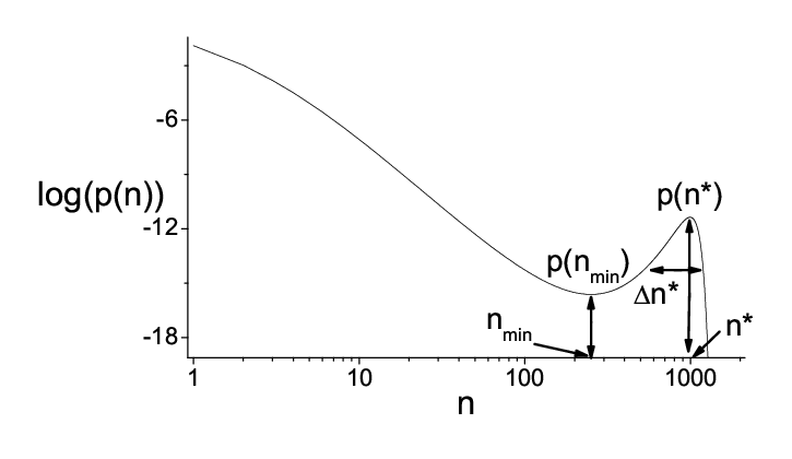
In this Section we study the characteristic features of the single site occupation distribution for the case of algebraically increasing hopping rate (3). In the condensed phase we expect this distribution to have the general form given in Figure 2. The distribution decays algebraically for intermediate and there is a peak in the distribution for large . The peak is associated with any condensates in the system. Our aim is to analyse the shape of this peak—its height, width and position. This information will determine the typical number of condensates present in the system and their typical occupancy.
3.1 Grand Canonical Analysis
To investigate the probability distribution in the condensed phase within the grand canonical ensemble we consider the effective potential defined through
| (13) |
| (14) |
Expanding for large and approximating for the sum as an integral yields
| (15) |
Since we are discussing condensation we consider only hopping rates with for which condensation is possible. In the condensed phase we expect the fugacity in the thermodynamic limit. Hence, one describes the fugacity as a function of the system size , such that
| (16) |
where as .
Putting all this together we obtain, for large and ,
| (17) |
which implies
| (18) |
where is a normalization constant.
We now identify the position of the peak which corresponds to a maximum of at . The condition
| (19) |
gives
| (20) |
Then can be eliminated in (17) resulting in
| (21) |
Looking for a solution such that scales as a power law of implies that . The leading order term in Equation (21) is the first term, and therefore
| (22) |
which implies that the leading order of is
| (23) |
The width of the peak at is given by
| (24) |
where
| (25) |
Using the above expression for , and noting that the first term of this expression is the leading one for large , we find
| (26) |
Since vanishes in the large limit we expect the canonical and grand canonical ensembles to be equivalent.
In order to calculate we note that the weight, , of the peak, that is the probability contained in the peak, is given by
| (27) |
In the condensed phase, the weight represents the fraction of sites which are condensate sites. The fraction of particles contained within the condensates is then . Since in the condensed phase this fraction is finite (i.e. ) we arrive at the condition
| (28) |
yielding
| (29) |
The weight of the peak, thus scales as
| (30) |
The above analysis of the scaling of the peak in implies the following condensation behaviour. We first note that the size of the condensates, (22), scales sub-linearly with the system size and therefore these are termed mesocondensates. The typical number of mesocondensates is which scales as up to logarithmic corrections. Therefore their number diverges sublinearly with .
We conclude by investigating the dip in to the left of denoted in Figure 2. As we discuss in Section 5 the dip probability is significant in determining the dynamics of the mesocondensates. Balancing the first two terms in the extremum condition (19) yields
| (31) |
Then, is readily evaluated as
| (32) |
In summary, the leading behaviour in the system size of the shape of peak is given by equations (22,26,29) and the dip by (31,32).
The analysis of this subsection has been carried out within the grand canonical ensemble. In the following subsection we will compare it with exact numerical results for finite systems obtained in the canonical ensemble. This will provide evidence that at least the leading behaviour for the scaling properties of the condensate peak are correctly given by (22,26,29).
3.2 Numerical results
For given by (3) and for , we plot in Figure 3 the exact for . This was computed by iterating the recursion relation (8) and using expression (7).

As expected the probability distribution exhibits a power law decay representing the fluid and a peak corresponding to the condensates. In the case, there is a single condensate containing particles which results in a peak location that scales as . For , the second moment is finite and the peak has a width of . For , the regime of anomalous fluctuations, the second moment diverges and the width of the peak scales as . For both regimes the peak is sharp in the sense that . It is clearly seen in Figure 3 that the peak for the case is sharper and at larger than for as expected from the above and (22,26,29).
In Figure 4 we present some snapshots of the occupations of the sites in the steady state as obtained from numerical simulations. It can be seen that while for (where (3) reduces to (1)) there is a single condensate, for the excess density above the critical value is distributed among a number of mesocondensates. It is the distribution of the occupations of these mesocondensates that the peak in describes.


Since the steady state properties of the distribution given in Section 3 were calculated in the grand canonical ensemble,we wish to compare the distribution obtained in the canonical ensemble with the one obtained in the grand canonical ensemble. In Figure 5 the probability distribution for the parameters , , , and was calculated numerically both in the grand-canonical ensemble (10) and in the canonical ensemble (7). It can be seen in Figure 5 that the distributions obtained form the two ensembles agree.

In Figure 6 we check that the grand canonical analysis yields the leading scaling properties of the peak calculated for the canonical distribution in finite size systems. In Figure 6(a), is plotted against . A slope which agrees with the expected value of is seen, confirming the dependence (29). In Figure 6(b) is plotted against . A slope which agrees with the expected value of is seen, confirming the dependence (22). The logarithmic corrections were not taken into account since the correction has negligible dependence.

In Figure 7 we check that the grand canonical analysis yields the leading scaling properties of the dip calculated for the canonical distribution in finite size systems. In Figure 7(a) the dip height is plotted against . A linear fit for the data with a slope of is seen, confirming the dependence (32). In Figure 7(b) the dip location is plotted against . A linear fit for the data with a slope of is seen, confirming the dependence (31).
We conclude that the steady state properties of the distribution given in Section 3 computed for the grand canonical ensemble are able to describe the properties in the canonical ensemble.
4 Analysis of condensation for exponentially increasing
In this section we consider the distribution corresponding to hopping rates (4). As can be seen in Figure 1, the hopping rate is basically given by the commonly used form (1) but with a rapid increase at . In turn this generates a sharp cut-off in at .
In the absence of the cut-off the condensate peak is at . Thus, we expect this still to be the case as long as . However, for densities above , and below , the density excess is distributed among two condensates each containing a maximum of particles. In general for densities , where is an integer, we would expect to have condensates. In other words the number of condensates is
| (33) |
where denotes the ceiling function which is the integer part of plus one. Thus, in contrast to the algebraic case, this model exhibits a finite number of extensive condensates.

For a density with integer , the condensed phase is composed of condensates with particles each. The structure of the condensed phase for noninteger is rather different. This is best illustrated by considering the case of two condensates: . The total number of particles in the two condensate sites is . Since the maximum occupation of a site is , the occupation of a condensate site fluctuates between and . A numerical simulation was carried out for , , and for which the expected number of condensates is . In Figure 8 the occupation of the two condensates is plotted as a function of time. Interestingly, the two condensates’ occupations fluctuate in an anticorrelated fashion between and around the mean occupation . As discussed in [12], the condensates interact and the role of the larger condensate is shared among the two condensates. This results in a distribution with two peaks with one centred at corresponding to condensates and the second corresponds to a single condensate containing the remaining particles. Here is the floor function, defined as the highest integer less than or equal to . The numerical results presented in section 4.2 confirm this behaviour.
In the following subsection we analyze the scaling properties of the condensates within the grand canonical ensemble. The grand canonical analysis of the ZRP with a sharp cut-off in occupation, as is the case here, leads to a peak in the distribution at the cut-off for any density above [4]. On the other hand the considerations of the previous paragraph indicate that the behaviour of the model with fixed number of particles (Canonical ensemble) is more complex with a distribution depending on . For example, as pointed out in the previous paragraph for the condensate peak is below the cut-off. We conclude that at densities for which is non-integer the grand canonical and canonical analyses do not yield the same scaling behaviour for the condensate. Thus we apply the grand canonical analysis for the case of integer where the condensate peak is at the cut-off point . In subsection 4.2 we numerically check the equivalence between the two ensembles in this case.
4.1 Grand Canonical Analysis
Following the same strategy as in subsection 3.1, one finds that for hopping rate (4)
| (34) |
which implies
| (35) |
where is a normalization constant.
The extremum condition on is
| (36) |
which implies
| (37) |
Looking for a solution such that implies that
| (38) |
where is a parameter which in principle can be determined. The leading order of is then
| (39) |
To calculate the width of the peak we note that
| (40) |
yielding
| (41) |
The condition yields
| (42) |
and the weight scales as .
The scaling behaviour of the peak in implies that the size of the condensates, (38), is extensive. Also, up to logarithmic corrections, the width of the peak (41) scales as the square root of its position. Thus the peak is sharp as in the usual condensation scenario associated with (1). The number of condensates is
| (43) |
where following our previous discussion we consider only densities for which is an integer. We will comment on other densities in the next subsection.
To locate the position of the dip, , in , we balance the first two terms in the extremum equation (36) which yields
| (44) |
and
| (45) |
4.2 Numerical results
We start by considering a case with integer . The results of numerical simulations for a system with hopping rates given by (4), size , , and are displayed in Figure 9. The probability distribution is given in Figure 9(a) where we can clearly see a narrow peak around . The simulation results are given by the circles and are compared to a numerical calculation of the exact canonical expression (7) represented by the full line. Since the critical density is 0.5 we expect the excess density to be distributed among two condensates. The occupation of each condensate is expected to be approximately equal to . A typical snapshot is presented in Figure 9(b) where the occupation of the lattice is plotted.

We now proceed to examine a case with non-integer . The results of numerical simulations for a system with hopping rates given by (4), size , , and are displayed in Figure 10. The probability distribution is given in Figure 10(a) where we can clearly see a rather broad peak around . The simulation results are given by the circles and are compared to a numerical calculation of the exact canonical expression (7) represented by the full line. Since the critical density is 0.5 we expect the excess density to be distributed among two condensates. Even though the occupation of each condensate fluctuates in time between and they spend the majority of the time in either and not in transition as can be seen in Figure 8. The resulting distribution has two peaks, one centred around and the second around , which yield the appearance of a single broader peak in Figure 10(a). A typical snapshot is presented in Figure 10(b) where the occupation of the lattice is plotted.


In Figure 11, we compare the numerical solution for the canonical distribution for (integer ) with that corresponding to and (where is non-integer) for , and . For the above parameters with a density of there is a single condensate corresponding to the single peak at . On the other hand for there are two condensates corresponding densities and , resulting in two distinct peaks in the distribution function. This is verified in Figure 11. Clearly, the results for non-integer do not agree with the grand canonical analysis in which there is a single peak corresponding to the multiple condensates.

Since the steady state properties of the distribution given in Section 4 were calculated in the grand canonical ensemble, in which the distribution exhibits only a single peak, we wish to compare the distribution obtained in the canonical ensemble with the one obtained in the grand canonical ensemble. In Figure 12 the probability distribution for the parameters , and was calculated numerically both in the grand-canonical ensemble (10) and in the canonical ensemble (7). In Figure 12(a) the distributions are compared for , a density in which a single condensate exits. In Figure 12(b) the distributions are compared for a density in which two condensates exist. It can be seen in Figure 12(a) and(b) that the distributions obtained form the two ensembles are not equivalent; they differ mostly at large . On the other hand, for small , namely in the fluid phase, the distributions obtained from the two ensembles agree.
For large occupations not only does the size dependent constraint on the number of particles affect the distribution but so does the size dependent term in the hopping rate (4). This endogenous size dependence yields a different form for the distribution at large . The height of the peak is the same in both ensembles for the two cases in Figures 12(a) and (b). However, the dip is different for the two ensembles even for the single condensate case in Figures 12(a). The scaling behaviour in the canonical ensemble of the distribution as a function of the system size can be calculated numerically using (7) and compared with the prediction in the grand-canonical ensemble (41,42,44,45).

In Figure 13 we check that in the case of integer the grand canonical analysis yields the leading scaling properties of the peak calculated for the canonical distribution in finite size systems. In the Figure, is plotted against . A slope which agrees with the expected value of is seen, confirming the dependence. However to test the logarithmic corrections more detailed numerical data are required.
For the non integer case the grand canonical analysis is not valid and as a result, the scaling relations developed using the grand canonical analysis do not hold. This was confirmed numerically using (7) to calculate the scaling in the canonical ensemble and comparing with the prediction in the grand-canonical ensemble (41,42,44,45).

As noted above in the discussion of Figure 12, the canonical and grand canonical distributions appear to differ in the dip region. However it may be that scaling is still correctly predicted by the grand canonical analysis. In Figure 14 we check that in the case of integer the grand canonical analysis yields the leading scaling properties of the dip calculated for the canonical distribution in finite size systems. In Figure 14(a) the dip location is plotted against . A linear fit for the data produced a slope of . In the figure the data is compared with a slope of corresponding to the scaling relation (44). In Figure 14(b) the dip height is plotted against . A linear fit for the data produced a slope of . In the figure the data is compared with a slope of corresponding to the scaling relation (45). This is not the case for the non integer since the dip is not well defined as the number of humps may be larger than one.
We conclude that for the case of integer the steady state properties of the distribution given in Section 4 computed for the grand canonical ensemble are able to describe the properties in the canonical ensemble. However, it seems as if the analysis breaks down for the case of non integer where the two descriptions are qualitatively different in the description of the condensates.
5 Dynamics
5.1 Condensate creation and evaporation timescales
We are interested in the dynamics of condensate formation for systems described by the hopping rates (3,4). Previous studies of condensate formation and dynamics for the case (1) have been carried out [6, 7, 13]. We identify two timescales associated with creation and evaporation of (meso)condensates in the system. To identify these timescales we note that the size of the (meso)condensates fluctuates around . These fluctuations are occasionally large enough to cause a condensate to evaporate. The typical time for a condensate to exist at a given site before it evaporates is termed the evaporation time and is denoted by . Once a condensate has evaporated the particles are redistributed among the other sites and this can result in formation of another condensate. The typical time that a given site exists in the fluid phase before a condensate is created at that site is termed the creation time and is denoted by .

In Figure 15 we display the time series of the occupation number of a typical site, for the algebraic case (3). One clearly sees sharp transitions between the fluid state and condensed state. By averaging over a long time series the evaporation and creation times may be evaluated. The results are illustrated in Figure 16. Similar plots for the exponential case are illustrated in Figure 18 for an integer number of condensates.

In order to estimate the evaporation time and creation time we use the Arrhenius law. As we have seen, the probability distribution of the occupation of a given site is described by an effective potential as illustrated in Figure 17. In the condensed phase exhibits two valleys. The left valley corresponds to fluid states and the right valley centred around corresponds to condensate states. The potential barrier centred around corresponds to the dip region in the probability distribution. Using the Arrhenius law, a condensate will form on the site once the occupation of the site crosses the barrier from the left to the right valley. The timescale for creation of a condensate is then proportional to the ratio of the probability of being in the fluid to the probability of being at the creation threshold . Thus, since the probability of being in the fluid is of the order of , we obtain
| (46) |
For the evaporation time of a condensate, the timescale is proportional to the ratio of the probability for a condensate, which is of the order of , to the probability of being at the evaporation threshold which is again at ,
| (47) |
Note that on general grounds the ratio of the two timescales has to satisfy
| (48) |
where is the ratio of the probabilities of a site being in a condensate or a fluid state. This follows from a steady-state condition that the rate per site of condensate creation is balanced by the rate per site of condensate evaporation . For small , (47) and (46) satisfy (48).

5.2 Numerical results for algebraically increasing case
For the algebraic hopping rate (3), the creation and evaporation times scale with the system size as
| (49) |
Using numerical simulations for for , and the evaporation time and creation time are plotted in Figure 16 as a function of the lattice size . In Figure 16(a) the evaporation time as a function of lattice size is compared on a double logarithmic scale to a linear slope of . In Figure 16(b) the creation time as a function of lattice size is compared on a double logarithmic scale to a linear slope of .
5.3 Numerical results for exponentially increasing case
In the following, we separate the discussion of the case of an integer from that of a non integer . To carry out an analogous analysis for the exponential hopping rate (4) with an integer . we require an expression for how scales with . As we have discussed, the hopping rate (4) is the same as the usual case (1) but with the introduction of a sharp cut-off at . Thus we expect to remain the same as that for (1) up to the condensate peak which takes place at . Therefore , as in the usual case (1), and . This estimate inserted into (46,47) yields the following leading behaviour for the creation and evaporation timescales in the exponential hopping rate case
| (50) |

We test the leading behaviour using numerical simulations for , and , which corresponds to an integer , the evaporation time and creation time are plotted in Figure 18 as a function of the lattice size . In Figure 18(a) the evaporation time as a function of lattice size is compared on a double logarithmic scale to a linear slope of . In Figure 18(b) the creation time as a function of lattice size is compared on a double logarithmic to a linear slope of . These results are consistent with the leading behaviour derived for the grand canonical ensemble (50), although more extensive simulations would be desirable.
On the other hand, for the case of non-integer the the leading behaviour of the creation time and of the evaporation time which were calculated within the grand canonical ensemble are invalid. The Arrhenius law approach is based on a distribution with a single peak and a single dip which is not the case for the non-integer as was shown above. Thus, for the non-integer not only is the distribution obtained within the grand canonical ensemble not valid, so is the framework in which we calculate the evaporation and creation times.
6 Conclusions
In this work we have shown how the introduction of non-monotonic hopping rates into the ZRP can produce a condensation transition into many condensates. The algebraic choice of hopping rate (3) results in mesocondensates whose number grows subextensively with system size . On the other hand, the exponential choice of hopping rate (4) can result in a finite number of extensive condensates.
Related condensation phenomena, which result in a large number of mesocondensates, have previously discussed in the context of non-conserving ZRP[9]. Thus our results imply that the steady states of such models can be described by a conserving ZRP with an effective hopping rate which is non-monotonic.
We have analysed the single-site distribution within the grand canonical ensemble and in particular analysed the scaling behaviour of the condensate peak. We have computed the scaling behaviour of the position, height, width of the peak and also the position and height of the dip between the condensate peak and the part of the distribution representing the fluid as illustrated in Figure 2.
In the case of algebraically increasing hopping rates (3) the predictions of the grand canonical analysis are well borne out by numerical computation within the canonical ensemble. Ignoring logarithmic corrections the scaling of the condensate peak is as follows: the position of the peak scales as ; the width scales as ; the height of the peak scales as , and the weight of the peak scales as . The behaviour of implies that the number of mesocondensates scales as . The peak is not sharp since only as a power of . Thus we term it a ‘weak peak’. The weak peak is similar to that determined in the analysis of a non-conserving ZRP [9].
For the exponential case (4) the situation is more subtle. For the case of integer values of , our numerical results suggest that the scaling predicted by the grand canonical analysis is correct even though the grand canonical and canonical distributions do not appear to coincide. The scaling of the condensate peak, excluding any logarithmic corrections, is as follows: the position of the peak scales as ; the width scales as ; the height of the peak scales as , and the weight of the peak scales as . The behaviour of implies that the number of mesocondensates is finite. In the exponential case the peak is ‘sharp’ since as a power of .
For the case of non-integer values of , on the other hand, it appears that the results of the grand canonical analysis break down.
It is of interest to compare the scaling form we have determined of the peak in corresponding to (meso)condensates to the usual scenario of condensation into a single site exhibited, for example, by the hopping rate (1). For the single condensate case, in [10, 11] the condensate peak, denoted in that work, has been computed. The scaling form of the peak is as follows: the position scales as ; the width scales as for and for ; the height scales as for and for ; and the weight of the peak scales as . The peak is sharp, as in the case we have studied of a finite number of condensates. However, in the case of a finite number of condensates, our grand canonical predictions for the scaling of the width and height of the peak do not depend on .
We note that for the usual single condensate scenario the results quoted above for were computed within the canonical ensemble [10, 11]. It would be of interest to see if our results can be recovered in a canonical calculation. Also, an analysis within the canonical ensemble is required to obtain the scaling form the condensate peak in the exponential case when is non-integer.
In studying the dynamics of the condensates we identified two timescales, one for the creation of a condensate at a given site and the other for the evaporation of a condensate at a given site. The scaling of these timescales with the system size has been studied within the phenomenological Arrhenius approach; how these timescales scale with system size is determined by the scaling of height of the dip and the weight of the condensate peak. We have found that the predictions compare well with numerical simulations in the algebraic case. In the exponential case the numerical results are consistent with the Arrhenius predictions, but more extensive simulations would be desirable.
References
References
- [1] P. Bialas, Z Burda, and D Johnston, Condensation in the Backgammon model, Nuclear Physics B, 493, 505, (1997)
- [2] M.R. Evans, Phase transitions in one-dimensional nonequilibrium systems, Braz. J. Phys. 30, 42 (2000)
- [3] F. Spitzer, Interaction of Markov processes, Adv. Math. 5, 246 (1970)
- [4] M.R. Evans and T. Hanney, Nonequilibrium statistical mechanics of the zero-range process and related models, J. Phys. A 38, R195 (2005)
- [5] C. Godrèche, From urn models to zero-range processes: statics and dynamics, in Ageing and the Glass Transition (Lecture Notes in Physics) ed M Henkel, M Pleimling and R Sanctuary (Berlin: Springer) (2006)
- [6] S. Großkinsky, G.M. Schütz and H. Spohn, Condensation in the zero-range process: stationary and dynamical properties, J. Stat. Phys. 113, 389 (2003)
- [7] C. Godrèche, Dynamics of condensation in zero-range processes, J. Phys. A 36, 6313 (2003)
- [8] A.G. Angel, M.R. Evans, E. Levine and D. Mukamel, Critical phase in non-conserving zero-range processes and equilibrium networks, Phys. Rev. E 72, 046132 (2005)
- [9] A.G. Angel, M.R. Evans, E. Levine and D. Mukamel, Criticality and condensation in a non-conserving zero-range process, J. Stat. Mech. P08017 (2007)
- [10] S.N. Majumdar, M. R. Evans and R. K. P. Zia, Nature of the Condensate in Mass Transport Models, Phys. Rev. Lett. 94, 180601 (2005)
- [11] M. R. Evans, S.N. Majumdar and R. K. P. Zia, Canonical Analysis of Condensation in Factorised Steady States, J. Stat. Phys. 123, 357 (2006)
- [12] Y Schwarzkopf, Masters Thesis, Weizmann Institute (2006)
- [13] C. Godrèche and J-M Luck, Dynamics of the condensate in zero-range processes, J. Phys. A 38, 7215 (2005)
- [14] S. Grosskinsky and G. M. Schutz, Discontinuous condensation transition and nonequivalence of ensembles in a zero-range process, arXiv.org:0801.1310, 2008