跳到论文正文
W Papers独立论文阅读器 arXiv:0801.4495 论文正文 计算阅读时间 · 0%
引用这篇论文根据当前论文元数据生成,正式投稿前建议核对。


License: arXiv.org perpetual non-exclusive license
arXiv:0801.4495v2 [hep-ph] 10 Jul 2008

Nucleon-to-Delta axial transition form factors in relativistic baryon chiral perturbation theory

L. S. Geng Affiliation:  Departamento de Física Teórica and IFIC, Centro Mixto Universidad de Valencia-CSIC, Institutos de Investigación de Paterna, Aptdo. 22085, 46071 Valencia, Spain    J. Martin Camalich Affiliation:  Departamento de Física Teórica and IFIC, Centro Mixto Universidad de Valencia-CSIC, Institutos de Investigación de Paterna, Aptdo. 22085, 46071 Valencia, Spain    L. Alvarez-Ruso Affiliation:  Departamento de Física Teórica and IFIC, Centro Mixto Universidad de Valencia-CSIC, Institutos de Investigación de Paterna, Aptdo. 22085, 46071 Valencia, Spain    M. J. Vicente Vacas Affiliation:  Departamento de Física Teórica and IFIC, Centro Mixto Universidad de Valencia-CSIC, Institutos de Investigación de Paterna, Aptdo. 22085, 46071 Valencia, Spain
August 24, 2026
Abstract

We report a theoretical study of the axial Nucleon to Delta(1232) (N→ΔN\rightarrow\Delta) transition form factors up to one-loop order in relativistic baryon chiral perturbation theory. We adopt a formalism in which the Δ\Delta couplings obey the spin-3/2 gauge symmetry and, therefore, decouple the unphysical spin-1/2 fields. We compare the results with phenomenological form factors obtained from neutrino bubble chamber data and in quark models.

pacs
23.40.Bw,12.39.Fe, 14.20.Gk

I Introduction

The axial N→Δ⁡(1232)N\rightarrow\Delta(1232) transition form factors play an important role in neutrino induced pion production on the nucleon, in particular at low energies [1, 2, 3, 4, 5]. These form factors have been parametrized phenomenologically to fit the ANL [6, 7] and BNL [8, 9] bubble-chamber data. In the past, the theoretical descriptions have been done using different approaches, for a review, see Ref. [10]. In recent years, there has been an increasing interest on these form factors. They have been calculated, for instance, using the chiral constituent quark model [11] and light cone QCD sum rules [12]. State of the art calculations within lattice QCD  [13, 14] have also become available. The possibility to extract the axial N→ΔN\rightarrow\Delta transition form factors using parity-violating electron scattering at Jefferson Lab [15] has been studied extensively [16, 17]. Present and future neutrino experiments could also provide further information on these form factors [18, 19, 20, 21, 22, 23].

Chiral perturbation theory, based on a simultaneous expansion of QCD Green functions in powers of the external momenta and of the quark masses, has achieved remarkable success in describing the dynamics of the light pseudoscalar mesons at low energies [24, 25, 26, 27]. The sector with one baryon is more problematic because, as was shown in Ref. [28], the systematic power counting is lost since the nucleon mass is not zero in the chiral limit. These problems were first handled in heavy baryon chiral perturbation theory (HBχ\chiPT), where nucleons are treated semi-relativistically [29, 30]. However, in certain cases, this approximation leads to convergence problems because the Green functions do not satisfy the analytical properties of the fully relativistic theory [31]. Recently, the systematic power counting has also been restored in the relativistic formulation through either the infrared [31] or the extended on-mass-shell regularization schemes [32, 33].

The explicit inclusion of the Δ\Delta in chiral perturbation theory requires a power counting that properly incorporates the Δ\Delta-NN mass difference, Δ≡MΔ−MN\varDelta\equiv M_{\Delta}-M_{N}, which is small compared to the chiral symmetry breaking scale. Two expansion schemes have been proposed. One is the small scale expansion [34] which considers Δ\varDelta to be of the same order as the other small scales in the theory, i.e., mπ∼p∼Δm_{\pi}\sim p\sim\varDelta. The other is the δ\delta expansion scheme, which counts Δ\varDelta differently depending on the energy domain [35]. Originally, the small scale expansion was used in HBχ\chiPT, while recently it has also been implemented in relativistic chiral perturbation theory [36, 37].

The vector N→ΔN\rightarrow\Delta transition form factors, important to understand e​NeN (γ​N\gamma N) reactions and the structure of the nucleon, have been calculated up to next-to-leading order in both the small scale expansion HBχ\chiPT [38, 39] and the δ\delta expansion relativistic baryon χ\chiPT [40, 41]. While axial form factors have been addressed in HBχ\chiPT [42], no calculation has been performed up to now within the relativistic framework. With lattice QCD results becoming available [13], it is timely to study the axial transition form factors within relativistic chiral perturbation theory.

In this paper, we use the relativistic baryon chiral perturbation theory, including explicitly the Δ\Delta resonance, to calculate the axial N→ΔN\rightarrow\Delta transition form factors up to order 3 in the δ\delta expansion. In sect. II, we briefly explain the power counting, the difference between the small scale expansion scheme and the δ\delta expansion scheme, write down the relevant Lagrangians up to next-to-next-to-leading order and the appropriate form of the Δ\Delta propagator. Loop calculations are performed in sect. III. In sect. IV, we discuss our results in terms of the low energy constants and loop functions. In sect. V we compare the results with both phenomenological parameterizations and other theoretical calculations. Summary and conclusions are given in sect. VI.

II Power counting, effective Lagrangians, and the Δ\Delta propagator

II.1 Power counting

A fundamental concept of χ\chiPT (as Effective Field Theory) is the power counting [24]. It provides a systematic organization of the effective Lagrangians and the corresponding loop-diagrams within a perturbative expansion in powers of (p/Λχ​SB)nχ​P​T(p/\Lambda_{\chi\mathrm{SB}})^{n_{\chi PT}}, where pp is a small momentum or scale and Λχ​SB\Lambda_{\chi\mathrm{SB}}, the chiral symmetry breaking scale. In χ\chiPT with pions and nucleons alone the chiral order of a diagram with LL loops, NπN_{\pi}(NNN_{N}) pion (nucleon) propagators, and VkV_{k} vertices from kkth-order Lagrangians is

nχ​P​T=4​L−2​Nπ−NN+∑kk​Vk.n_{\chi PT}=4L-2N_{\pi}-N_{N}+\sum_{k}kV_{k}\,. (1)

However, in the covariant theory this rule is violated in loops by lower-order analytical pieces [28]. This power counting can be recovered by adopting non-trivial renormalization schemes, where the lower-order power-counting breaking pieces of the loop results are systematically absorbed into the available counter-terms [31, 33]. A detailed discussion of the renormalization scheme adopted in the present work will be presented together with our main results in section IV.

If the Δ\Delta resonance is explicitly considered, things become more complicated because its excitation energy, Δ≡MΔ−MN∼0.3\varDelta\equiv M_{\Delta}-M_{N}\sim 0.3 GeV, is small compared to the chiral symmetry breaking scale Λχ​SB=4​π​fπ∼1\Lambda_{\chi\mathrm{SB}}=4\pi f_{\pi}\sim 1 GeV. Therefore, there are two small parameters in the theory, i.e.,

ε=mπ/Λχ​SBandδ=Δ/Λχ​SB.\varepsilon=m_{\pi}/\Lambda_{\chi\mathrm{SB}}\quad\mbox{and}\quad\delta=\varDelta/\Lambda_{\chi\mathrm{SB}}. (2)

Over the past few years, two different expansion schemes have been proposed, the small scale expansion and the δ\delta expansion. In the small scale expansion [34], one has mπ∼Δ∼p∼𝒪⁡(ϵ)m_{\pi}\sim\varDelta\sim p\sim\mathcal{O}(\epsilon). In the δ\delta-expansion [35], to maintain the scale hierarchy mπ≪Δ≪Λχ​SBm_{\pi}\ll\varDelta\ll\Lambda_{\chi\mathrm{SB}}, mπ/Λχ​SBm_{\pi}/\Lambda_{\chi\mathrm{SB}} is counted as δ2\delta^{2}. In this scheme, the power counting depends on the energy domain under study: p∼mπp\sim m_{\pi} or p∼Δp\sim\varDelta.

For the study of N→ΔN\rightarrow\Delta axial transition form factors in the energy region p∼Δp\sim\varDelta, the order of a graph with LL loops, VkV_{k} vertices of dimension kk, NπN_{\pi} pion propagators, NNN_{N} nucleon propagators, NΔN_{\Delta} Delta propagators, the power-counting index nn is given by:

n=nχ​PT−NΔ.n=n_{\chi\mathrm{PT}}-N_{\Delta}. (3)

For a more general discussion, see Ref. [43].

In the present work, we adopt the δ\delta expansion scheme. As can be seen in the following sections, the differences between these two schemes in our case come from vertices proportional to mπ2m_{\pi}^{2}, which count as δ4\delta^{4} in the δ\delta expansion and, therefore, have been neglected.

II.2 Chiral Lagrangians

In this section, we write down the relevant N​NNN, N​ΔN\Delta, and Δ​Δ\Delta\Delta Lagrangians and pay special attention to the Δ\Delta couplings and the spin-3/2 gauge symmetry.

II.2.1 Pion-nucleon and pion-pion Lagrangians

The lowest order pion-nucleon Lagrangian has the following form:

ℒπ​N(1)=N¯​(i​γμ​Dμ−MN−gA2​γμ​γ5​uμ)​N,\mathcal{L}^{(1)}_{\pi N}=\bar{N}(i\gamma^{\mu}D_{\mu}-M_{N}-\frac{g_{A}}{2}\gamma^{\mu}\gamma^{5}u_{\mu})N, (4)

where MNM_{N} and gAg_{A} are the nucleon mass and the axial-vector coupling at the chiral limit, DμD_{\mu} is the covariant derivative

Dμ​N=∂μN+[Γμ,N],D_{\mu}N=\partial_{\mu}N+[\Gamma_{\mu},N], (5)
Γμ=12{u†(∂μ−irμ)u+u(∂μ−ilμ)u†},\Gamma_{\mu}=\frac{1}{2}\left\{u^{\dagger}(\partial_{\mu}-ir_{\mu})u+u(\partial_{\mu}-il_{\mu})u^{\dagger}\right\}, (6)

and uμu_{\mu} the axial current defined as

uμ=i{u†(∂μ−irμ)u−u(∂μ−ilμ)u†}.u_{\mu}=i\left\{u^{\dagger}(\partial_{\mu}-ir_{\mu})u-u(\partial_{\mu}-il_{\mu})u^{\dagger}\right\}. (7)

In the above definitions, rμ=vμ+aμr_{\mu}=v_{\mu}+a_{\mu}, lμ=vμ−aμl_{\mu}=v_{\mu}-a_{\mu} with vμ=τσ​vμσ/2v_{\mu}=\tau^{\sigma}v^{\sigma}_{\mu}/2 and aμ=τσ​aμσ/2a_{\mu}=\tau^{\sigma}a^{\sigma}_{\mu}/2 the external vector and axial currents, where τσ\tau^{\sigma} are the Pauli matrices. The matrix uu incorporates the pion fields

u2=U=exp⁡[i​Φfπ],u^{2}=U=\exp\left[i\frac{\Phi}{f_{\pi}}\right], (8)
Φ=τσ​πσ=(π02​π+2​π−−π0),\Phi=\tau_{\sigma}\pi^{\sigma}=\left(\begin{array}[]{cc}\pi^{0}&\sqrt{2}\pi^{+}\\ \sqrt{2}\pi^{-}&-\pi^{0}\end{array}\right), (9)

with fπf_{\pi} being the pion decay constant in the chiral limit.

The leading order pion-pion Lagrangian has the following form:

ℒπ​π(2)=fπ24​Tr​[∇μU​(∇μU)†]+fπ24​Tr​[χ​U†+U​χ†],\mathcal{L}^{(2)}_{\pi\pi}=\frac{f_{\pi}^{2}}{4}\mathrm{Tr}\left[\nabla_{\mu}U(\nabla^{\mu}U)^{\dagger}\right]+\frac{f_{\pi}^{2}}{4}\mathrm{Tr}\left[\chi U^{\dagger}+U\chi^{\dagger}\right], (10)

where

∇μU=∂μU−i​rμ​U+i​U​lμ\nabla_{\mu}U=\partial_{\mu}U-ir_{\mu}U+iUl_{\mu} (11)

with χ=diag⁡(mπ2,mπ2)\chi=\mathrm{diag}(m^{2}_{\pi},m^{2}_{\pi}).

II.2.2 Nucleon-Delta and Delta-Delta Lagrangians

The Δ⁡(1232)\Delta(1232) is a spin-3/2 resonance and, therefore, its spin content can be described in terms of the Rarita-Schwinger (RS) field Δμ\Delta_{\mu}, where μ\mu is the Lorentz index.11 1 We follow Ref. [43] and write the Lagrangians for the spin-3/2 isospin-3/2 Δ\Delta isobar in terms of the Rarita-Schwinger (vector-spinor) isoquartet field Δμ=(Δ+⁣+,Δ+,Δ0,Δ−)μt\Delta_{\mu}=(\Delta^{++},\Delta^{+},\Delta^{0},\Delta^{-})_{\mu}^{t}, which is connected to the isospurion representation of Ref. [34] through Δμa=−Ta​Δμ\Delta^{a}_{\mu}=-T^{a}\Delta_{\mu} where TaT^{a} are the isospin 1/2 to 3/2 matrices satisfying TaTb†=δa​b−1/3τaτbT^{a}T^{b\dagger}=\delta^{ab}-1/3\tau^{a}\tau^{b}, as given in Appendix A. With this rule, the on-shell equivalent form of our consistent couplings can be easily identified with those of Refs. [34, 44]. This field, however, contains unphysical spin-1/2 components. They are allowed for the description of off-shell Delta’s, but the physical results should not depend on them. In order to tackle this problem, we follow Refs. [45, 43] and adopt the consistent couplings, which are gauge-invariant under the transformation

Δμ​(x)→Δμ​(x)+∂μϵ⁡(x).\Delta_{\mu}(x)\rightarrow\Delta_{\mu}(x)+\partial_{\mu}\epsilon(x). (12)

A remarkable consequence of the use of the spin-3/2 gauge symmetric couplings is that it leads to a natural decoupling of the propagation of the spin-1/2 fields.

In the following we give the N​ΔN\Delta and Δ​Δ\Delta\Delta Lagrangians relevant to this work. The lowest order Lagrangians in the resonance region are22 2 If one Δ\Delta is put on-shell, the Δ\Delta-Δ\Delta Lagrangian is equivalent to that of Pascalutsa et al. [43]: ℒΔ​Δ(1)=−HA2​MΔ​ϵμ​ν​ρ​σ​Δ¯μ​𝒯a​(∂ρΔν)​ωσa+H.c..\mathcal{L}_{\Delta\Delta}^{(1)}=-\frac{H_{A}}{2M_{\Delta}}\epsilon^{\mu\nu\rho\sigma}\bar{\Delta}_{\mu}\mathcal{T}^{a}(\partial_{\rho}\Delta_{\nu})\omega_{\sigma}^{a}+\mathrm{H.c.}.

ℒN​Δ(1)=−i​hA2​MΔ​N¯​Ta​γμ​ν​λ​(∂μΔν)​ωλa+H.c.,\mathcal{L}_{N\Delta}^{(1)}=-\frac{ih_{A}}{2M_{\Delta}}\bar{N}T^{a}\gamma^{\mu\nu\lambda}(\partial_{\mu}\Delta_{\nu})\omega^{a}_{\lambda}+\mathrm{H.c.}, (13)
ℒΔ​Δ(1)=HA2​MΔ2​∂mΔ¯b​γℓ​b​m​γμ​γ5​𝒯a​ωμa​γℓ​c​n​∂nΔc,\mathcal{L}_{\Delta\Delta}^{(1)}=\frac{H_{A}}{2M^{2}_{\Delta}}\partial_{m}\bar{\Delta}_{b}\gamma^{\ell bm}\gamma^{\mu}\gamma^{5}\mathcal{T}^{a}\omega^{a}_{\mu}\gamma_{\ell cn}\partial^{n}\Delta^{c}, (14)

where ωλa=12Tr(τauλ)=−1fπ∂λπa+aλa+⋯\omega^{a}_{\lambda}=\frac{1}{2}\mathrm{Tr}\left(\tau^{a}u_{\lambda}\right)=-\frac{1}{f_{\pi}}\partial_{\lambda}\pi^{a}+a^{a}_{\lambda}+\cdots, TaT^{a} and 𝒯a\mathcal{T}^{a} are the isospin 1/2 to 3/2 and 3/2 to 3/2 transition matrices, and γμ​ν​λ\gamma^{\mu\nu\lambda} is the totally antisymmetric gamma matrix product as given in Appendix A. At second order, there are four terms, i.e.,33 3 In our study of the axial form factors up to one-loop order the δ(2)\delta^{(2)} and δ(3)\delta^{(3)} Lagrangians only concern on-shell Δ\Delta’s. Therefore, they are the same in the consistent coupling scheme of Pascalutsa et al. as those conventional Lagrangians in Refs. [34, 44].

ℒN​Δ(2)\displaystyle\mathcal{L}_{N\Delta}^{(2)} =\displaystyle= −d1MΔ​N¯​Ta​(∂μΔν)​f−a,μ​ν−i​d2​N¯​Ta​f−a,μ​ν​γμ​Δν−i​d3​N¯​Ta​ωa,μ​ν​γμ​Δν\displaystyle-\frac{d_{1}}{M_{\Delta}}\bar{N}T^{a}(\partial_{\mu}\Delta_{\nu})f_{-}^{a,\mu\nu}-id_{2}\bar{N}T^{a}f_{-}^{a,\mu\nu}\gamma_{\mu}\Delta_{\nu}-id_{3}\bar{N}T^{a}\omega^{a,\mu\nu}\gamma_{\mu}\Delta_{\nu} (15)
−d4MΔ​N¯​Ta​(∂μΔν)​ωa,μ​ν+H.c.,\displaystyle-\frac{d_{4}}{M_{\Delta}}\bar{N}T^{a}(\partial_{\mu}\Delta_{\nu})\omega^{a,\mu\nu}+\mathrm{H.c.},

while at third order, there are seven terms44 4 In the small scale expansion scheme, there are two more terms at this order proportional to mπ2m_{\pi}^{2}, i.e., −f8​N¯​Ta​ωνa​Tr​[χ+]​Δν−f9​i​N¯​Ta​[Dν,χ−a]​Δν,-f_{8}\bar{N}T^{a}\omega_{\nu}^{a}\mathrm{Tr}[\chi_{+}]\Delta^{\nu}-f_{9}i\bar{N}T^{a}\left[D_{\nu},\chi^{a}_{-}\right]\Delta^{\nu}, where χ+\chi_{+} and χ−\chi_{-} are external scalar and pseudoscalar sources.

ℒN​Δ(3)\displaystyle\mathcal{L}_{N\Delta}^{(3)} =\displaystyle= −f1N¯TaΔν∂μf−a,μ​ν−f2N¯TaΔν∂μωa,μ​ν+if3MΔN¯Ta∂μf−a,α​νγν∂μΔα\displaystyle-f_{1}\bar{N}T^{a}\Delta_{\nu}\partial_{\mu}f_{-}^{a,\mu\nu}-f_{2}\bar{N}T^{a}\Delta_{\nu}\partial_{\mu}\omega^{a,\mu\nu}+i\frac{f_{3}}{M_{\Delta}}\bar{N}T^{a}\partial^{\mu}f_{-}^{a,\alpha\nu}\gamma_{\nu}\partial_{\mu}\Delta_{\alpha} (16)
+if4MΔN¯Ta∂μf−a,α​νγμ∂νΔα−if5MΔN¯Ta∂μωa,ν​αγμ∂νΔα\displaystyle+i\frac{f_{4}}{M_{\Delta}}\bar{N}T^{a}\partial^{\mu}f_{-}^{a,\alpha\nu}\gamma_{\mu}\partial_{\nu}\Delta_{\alpha}-i\frac{f_{5}}{M_{\Delta}}\bar{N}T^{a}\partial^{\mu}\omega^{a,\nu\alpha}\gamma_{\mu}\partial_{\nu}\Delta_{\alpha}
+f6MΔ2N¯Ta∂μfa,ν​α−∂μ∂νΔα+f7MΔ2N¯Ta∂μωa,ν​α∂μ∂νΔα+H.c.,\displaystyle+\frac{f_{6}}{M^{2}_{\Delta}}\bar{N}T^{a}\partial^{\mu}f^{a,\nu\alpha}_{-}\partial_{\mu}\partial_{\nu}\Delta_{\alpha}+\frac{f_{7}}{M^{2}_{\Delta}}\bar{N}T^{a}\partial^{\mu}\omega^{a,\nu\alpha}\partial_{\mu}\partial_{\nu}\Delta_{\alpha}+\mathrm{H.c.},

where ωμ​νa=12​Tr​(τa​[Dμ,uν])\omega^{a}_{\mu\nu}=\frac{1}{2}\mathrm{Tr}(\tau^{a}[D_{\mu},u_{\nu}]), f−a,μ​ν=∂μaa,ν−∂νaa,μf_{-}^{a,\mu\nu}=\partial^{\mu}a^{a,\nu}-\partial^{\nu}a^{a,\mu}. As we will see later, the δ(2)\delta^{(2)} and δ(3)\delta^{(3)} low-energy constants (LEC) contribute to the form factors only in particular combinations; therefore, the number of independent parameters is smaller than the one appearing in the above Lagrangians.

II.3 Spin-3/2 propagator

The most general spin-3/2 free field propagator in DD dimensions has the following form [36, 46]:

Sα​β​(p)\displaystyle S^{\alpha\beta}(p) =\displaystyle= p/+MΔMΔ2−p2[gα​β−γα​γβ(D−1)+(1−ζ)(ζp/+MΔ)(D−1)​(ζ2​p2−MΔ2)(γαpβ−γβpα)\displaystyle\frac{p\!\!\!/\penalty+M_{\Delta}}{M_{\Delta}^{2}-p^{2}}\bigg[g^{\alpha\beta}-\frac{\gamma^{\alpha}\gamma^{\beta}}{(D-1)}+\frac{(1-\zeta)(\zeta p\!\!\!/\penalty+M_{\Delta})}{(D-1)(\zeta^{2}p^{2}-M_{\Delta}^{2})}(\gamma^{\alpha}p^{\beta}-\gamma^{\beta}p^{\alpha}) (17)
+(D−2)​(1−ζ2)​pα​pβ(D−1)​(ζ2​p2−MΔ2)],\displaystyle\hskip 227.62204pt+\frac{(D-2)(1-\zeta^{2})p^{\alpha}p^{\beta}}{(D-1)(\zeta^{2}p^{2}-M_{\Delta}^{2})}\bigg],

where ζ\zeta is the spin-3/2 gauge-fixing parameter. In the case of ζ=0\zeta=0, the above propagator corresponds to the usual Rarita-Schwinger propagator

Sα​β​(p)=p/+MΔMΔ2−p2​[gα​β−γα​γβ(D−1)−1(D−1)​MΔ​(γα​pβ−γβ​pα)−(D−2)​pα​pβ(D−1)​MΔ2];S^{\alpha\beta}(p)=\frac{p\!\!\!/\penalty+M_{\Delta}}{M_{\Delta}^{2}-p^{2}}\left[g^{\alpha\beta}-\frac{\gamma^{\alpha}\gamma^{\beta}}{(D-1)}-\frac{1}{(D-1)M_{\Delta}}(\gamma^{\alpha}p^{\beta}-\gamma^{\beta}p^{\alpha})-\frac{(D-2)p^{\alpha}p^{\beta}}{(D-1)M_{\Delta}^{2}}\right]; (18)

while in the case of ζ=∞\zeta=\infty, it becomes

Sα​β​(p)=p/+MΔMΔ2−p2​𝒫3/2α​β​(p)S^{\alpha\beta}(p)=\frac{p\!\!\!/\penalty+M_{\Delta}}{M_{\Delta}^{2}-p^{2}}\mathcal{P}^{\alpha\beta}_{3/2}(p) (19)

with the covariant spin-3/2 projection operator defined by

𝒫3/2α​β(p)=gα​β−γα​γβ(D−1)−1(D−1)​p2(p/γαpβ+pαγβp/)−(D−4)​pα​pβ(D−1)​p2.\mathcal{P}^{\alpha\beta}_{3/2}(p)=g^{\alpha\beta}-\frac{\gamma^{\alpha}\gamma^{\beta}}{(D-1)}-\frac{1}{(D-1)p^{2}}\left(p\!\!\!/\penalty\gamma^{\alpha}p^{\beta}+p^{\alpha}\gamma^{\beta}p\!\!\!/\penalty\right)-\frac{(D-4)p^{\alpha}p^{\beta}}{(D-1)p^{2}}. (20)

It should be stressed that due to the spin-3/2 gauge symmetric nature of the consistent couplings, our results do not depend on the particular value of the gauge-fixing parameter ζ\zeta.

Refer to caption
Figure 1: Feynman diagrams contributing to the axial N→ΔN\rightarrow\Delta transition form factors up to δ(3)\delta^{(3)}. The double, solid, and dashed lines correspond to the Delta, nucleon, and pion, while the wiggly line denotes the external axial source.

III The N→ΔN\rightarrow\Delta axial transition form factors

The N→ΔN\rightarrow\Delta axial transition form factors can be parameterized in terms of the usually called Adler form factors [1, 47]:

⟨Δα+​(p′)|−Aα​μ,3|P⁡(p)⟩\displaystyle\langle\Delta^{+}_{\alpha}(p^{\prime})|-A^{\alpha\mu,3}|P(p)\rangle =\displaystyle= Δ¯α+(p′){C3A​(q2)MN(gα​μγ⋅q−qαγμ)+C4A​(q2)MN2(q⋅p′gα​μ−qαp′μ)\displaystyle\bar{\Delta}^{+}_{\alpha}(p^{\prime})\bigg\{\frac{C^{A}_{3}(q^{2})}{M_{N}}\big(g^{\alpha\mu}\gamma\cdot q-q^{\alpha}\gamma^{\mu}\big)+\frac{C^{A}_{4}(q^{2})}{M^{2}_{N}}\big(q\cdot p^{\prime}g^{\alpha\mu}-q^{\alpha}p^{\prime\mu}\big) (21)
+C5A(q2)gα​μ+C6A​(q2)MN2qαqμ}N,\displaystyle\hskip 85.35826pt+C^{A}_{5}(q^{2})g^{\alpha\mu}+\frac{C^{A}_{6}(q^{2})}{M^{2}_{N}}q^{\alpha}q^{\mu}\bigg\}N,

where Aα​μ,3A^{\alpha\mu,3} is the third isospin component of the axial current.

All the diagrams contributing to the N→ΔN\rightarrow\Delta axial transition form factors up to δ(3)\delta^{(3)} are displayed in Fig. 1.55 5 We do not have the diagrams (c), (d), (e), and (f) of Fig. 1 of Ref. [42], that correspond to tadpole diagrams where a pion loop couples to either the A​N​ΔAN\Delta (π​N​Δ\pi N\Delta, A​πA\pi) vertices, or the pion fields, because the contribution of those diagrams are of higher-order in the δ\delta expansion scheme. Two Kroll-Ruderman like diagrams are not shown since the one with an internal nucleon and a A​π​N​NA\pi NN vertex is zero and the other one with an internal Δ\Delta and a A​π​Δ​ΔA\pi\Delta\Delta vertex contributes as a real constant, which is irrelevant to the present study due to the adopted renormalization scheme. The calculation of the tree-level diagrams [Fig. 1(a)] is straightforward:

A(a)α​μ,3\displaystyle A^{\alpha\mu,3}_{(a)} =\displaystyle= 23[−hA2gα​μ−d1MΔ(p′⋅qgα​μ−qαp′μ)−d2(γ⋅qgα​μ−qαγμ)−d3γ⋅qgα​μ\displaystyle\sqrt{\frac{2}{3}}\Bigg[-\frac{h_{A}}{2}g^{\alpha\mu}-\frac{d_{1}}{M_{\Delta}}(p^{\prime}\cdot qg^{\alpha\mu}-q^{\alpha}p^{\prime\mu})-d_{2}(\gamma\cdot qg^{\alpha\mu}-q^{\alpha}\gamma^{\mu})-d_{3}\gamma\cdot qg^{\alpha\mu} (22)
−d4MΔp′⋅qgα​μ+f1(q2gα​μ−qαqμ)+f2q2gα​μ+f3MΔp′⋅q(γ⋅qgα​μ−qαγμ)\displaystyle\hskip 36.98866pt-\frac{d_{4}}{M_{\Delta}}p^{\prime}\cdot qg^{\alpha\mu}+f_{1}(q^{2}g^{\alpha\mu}-q^{\alpha}q^{\mu})+f_{2}q^{2}g^{\alpha\mu}+\frac{f_{3}}{M_{\Delta}}p^{\prime}\cdot q(\gamma\cdot qg^{\alpha\mu}-q^{\alpha}\gamma^{\mu})
+f4MΔγ⋅q(p′⋅qgα​μ−qαp′μ)+f5MΔγ⋅qp′⋅qgα​μ+f6MΔ2p′⋅q(p′⋅qgα​μ−qαp′μ)\displaystyle\hskip 36.98866pt+\frac{f_{4}}{M_{\Delta}}\gamma\cdot q\left(p^{\prime}\cdot qg^{\alpha\mu}-q^{\alpha}p^{\prime\mu}\right)+\frac{f_{5}}{M_{\Delta}}\gamma\cdot qp^{\prime}\cdot qg^{\alpha\mu}+\frac{f_{6}}{M^{2}_{\Delta}}p^{\prime}\cdot q(p^{\prime}\cdot qg^{\alpha\mu}-q^{\alpha}p^{\prime\mu})
+f7MΔ2p′⋅qp′⋅qgα​μ],\displaystyle\hskip 36.98866pt+\frac{f_{7}}{M^{2}_{\Delta}}p^{\prime}\cdot qp^{\prime}\cdot qg^{\alpha\mu}\Bigg],

where p′p^{\prime}, pp, and qq are the momenta of the Δ\Delta, the nucleon, and the external source. We assume that both the external nucleon and Δ\Delta are on-shell, which yields p′⋅q/MΔ=(MΔ2−MN2+q2)/(2​MΔ)≈Δp^{\prime}\cdot q/M_{\Delta}=(M^{2}_{\Delta}-M^{2}_{N}+q^{2})/(2M_{\Delta})\approx\varDelta and γ⋅q=MΔ−MN=Δ\gamma\cdot q=M_{\Delta}-M_{N}=\varDelta, where we have neglected the q2q^{2} and Δ2\varDelta^{2} terms which, strictly speaking, are of higher order than the chiral order of the corresponding Lagrangian.

In the following we explicitly show how to calculate the loop diagrams:

Diagram Fig. 1(c) reads

A(c)α​μ,3=−23​[hA​gA2(8​π​fπ)2​1MΔ]​i​G(c)α​μA^{\alpha\mu,3}_{(c)}=-\sqrt{\frac{2}{3}}\left[\frac{h_{A}g_{A}^{2}}{(8\pi f_{\pi})^{2}}\frac{1}{M_{\Delta}}\right]iG^{\alpha\mu}_{(c)} (23)

with

i​G(c)α​μ=(2​π​μ)4−D​∫dD​ki​π2​p′bγb​α​ckc[p′/−k/+MN]γμγ5[p/−k/+MN]k/γ5[k2−mπ2+i​ϵ]​[(p−k)2−MN2+i​ϵ]​[(p′−k)2−MN2+i​ϵ],iG^{\alpha\mu}_{(c)}=(2\pi\mu)^{4-D}\int\frac{d^{D}k}{i\pi^{2}}\frac{p^{\prime}_{b}\gamma^{b\alpha c}k_{c}\left[p^{\prime}\!\!\!\!/\penalty-k\!\!\!/\penalty+M_{N}\right]\gamma^{\mu}\gamma_{5}\left[p\!\!\!/\penalty-k\!\!\!/\penalty+M_{N}\right]k\!\!\!/\penalty\gamma_{5}}{[k^{2}-m_{\pi}^{2}+i\epsilon][(p-k)^{2}-M_{N}^{2}+i\epsilon][(p^{\prime}-k)^{2}-M_{N}^{2}+i\epsilon]}, (24)

where μ\mu, the renormalization scale, is set to be MΔM_{\Delta}.

Diagram Fig. 1(e) reads

A(e)α​μ,3=56​23​[gA​hA​HA(8​π​fπ)2​1MΔ2]​i​G(e)α​μ,A^{\alpha\mu,3}_{(e)}=\frac{5}{6}\sqrt{\frac{2}{3}}\left[\frac{g_{A}h_{A}H_{A}}{(8\pi f_{\pi})^{2}}\frac{1}{M^{2}_{\Delta}}\right]iG^{\alpha\mu}_{(e)}, (25)

with

i​G(e)α​μ=(2​π​μ)4−D​∫dD​ki​π2​iϵα​a​b​cp′bkcSa​d(p′−k)γe​d​μ(p′−k)e(p/−k/+MN)k/γ5[k2−mπ2+i​ϵ]​[(p−k)2−MN2+i​ϵ].iG^{\alpha\mu}_{(e)}=(2\pi\mu)^{4-D}\int\frac{d^{D}k}{i\pi^{2}}\frac{i\epsilon^{\alpha abc}p^{\prime}_{b}k_{c}S_{ad}(p^{\prime}-k)\gamma^{ed\mu}(p^{\prime}-k)_{e}(p\!\!\!/\penalty-k\!\!\!/\penalty+M_{N})k\!\!\!/\penalty\gamma_{5}}{[k^{2}-m_{\pi}^{2}+i\epsilon][(p-k)^{2}-M_{N}^{2}+i\epsilon]}. (26)

Diagram Fig. 1(g) reads

A(g)α​μ,3=16​23​[hA3(8​π​fπ)2​1MΔ3]​i​G(g)α​μA^{\alpha\mu,3}_{(g)}=\frac{1}{6}\sqrt{\frac{2}{3}}\left[\frac{h^{3}_{A}}{(8\pi f_{\pi})^{2}}\frac{1}{M^{3}_{\Delta}}\right]iG^{\alpha\mu}_{(g)} (27)

with

i​G(g)α​μ=(2​π​μ)4−D​∫dD​ki​π2​p′aγa​α​bkb(p′/−k/−MN)γc​β​μ(p−k)cSβ​γ(p−k)γd​γ​e(p−k)dke[k2−mπ2+i​ϵ]​[(p′−k)2−MN2+i​ϵ].iG^{\alpha\mu}_{(g)}=(2\pi\mu)^{4-D}\int\frac{d^{D}k}{i\pi^{2}}\frac{p^{\prime}_{a}\gamma^{a\alpha b}k_{b}(p^{\prime}\!\!\!\!/\penalty-k\!\!\!/\penalty-M_{N})\gamma^{c\beta\mu}(p-k)_{c}S_{\beta\gamma}(p-k)\gamma^{d\gamma e}(p-k)_{d}k_{e}}{[k^{2}-m_{\pi}^{2}+i\epsilon][(p^{\prime}-k)^{2}-M_{N}^{2}+i\epsilon]}. (28)

Diagram Fig. 1(i) reads

A(i)α​μ,3=59​23​[hA​HA2(8​π​fπ)2​1MΔ4]​i​G(i)α​μA^{\alpha\mu,3}_{(i)}=\frac{5}{9}\sqrt{\frac{2}{3}}\left[\frac{h_{A}H^{2}_{A}}{(8\pi f_{\pi})^{2}}\frac{1}{M^{4}_{\Delta}}\right]iG^{\alpha\mu}_{(i)} (29)

with

i​G(i)α​μ\displaystyle iG^{\alpha\mu}_{(i)} =\displaystyle= (2​π​μ)4−D​∫dD​ki​π2\displaystyle(2\pi\mu)^{4-D}\int\frac{d^{D}k}{i\pi^{2}} (30)
×\displaystyle\times i​ϵα​a​ρ​σ​(p′−k)ρ​kσ​Sa​b​(p′−k)​γl​b​m​γμ​γ5​γl​c​n​(p′−k)m​(p−k)n​Sc​d​(p−k)​γf​d​g​(p−k)f​kg[k2−mπ2+i​ϵ].\displaystyle\frac{i\epsilon^{\alpha a\rho\sigma}(p^{\prime}-k)_{\rho}k_{\sigma}S_{ab}(p^{\prime}-k)\gamma^{lbm}\gamma^{\mu}\gamma^{5}\gamma_{lcn}(p^{\prime}-k)_{m}(p-k)^{n}S^{cd}(p-k)\gamma_{fdg}(p-k)^{f}k^{g}}{[k^{2}-m_{\pi}^{2}+i\epsilon]}.

In the above equations, Sμ​ν​(p)S^{\mu\nu}(p) is the spin-3/2 propagator defined in Eq. (17). Since the couplings we used are spin-3/2 gauge symmetric, our results do not depend on the specific value of the gauge fixing parameter.

These loop functions are quite complicated, particularly the ones including Δ\Delta internal lines. In practice, we adopt the conventional Feynman parametrization method (see Appendix B) and calculate these loop functions numerically. The manipulation of the Dirac algebra has been performed independently with FORM [48] and FeynCalc [49]. The resulting Feynman parameter integrals are listed in Appendix C. Whenever possible, the numerical results have been checked using the FF library [50] through the LoopTools interface [51].

The one-loop results contain only four different Lorentz structures (due to the constraints Δ¯α​γα=0\bar{\Delta}_{\alpha}\gamma^{\alpha}=0 and Δ¯α​p′α=0\bar{\Delta}_{\alpha}p^{\prime\alpha}=0), i.e., γμ​qα\gamma^{\mu}q^{\alpha}, qα​p′μq^{\alpha}p^{\prime\mu}, gα​μg^{\alpha\mu}, and qα​qμq^{\alpha}q^{\mu}. In accordance with the Adler formulation of Eq. (21), we can identify the corresponding Lorentz structures and group the results as

A(c)α​μ,3+A(e)α​μ,3+A(g)α​μ,3+A(i)α​μ,3\displaystyle A^{\alpha\mu,3}_{(c)}+A^{\alpha\mu,3}_{(e)}+A^{\alpha\mu,3}_{(g)}+A^{\alpha\mu,3}_{(i)} =\displaystyle= 23[g3(q2)(gα​μγ⋅q−qαγμ)+g4(q2)(q⋅p′gα​μ−qαp′μ)\displaystyle\sqrt{\frac{2}{3}}\bigg[g_{3}(q^{2})\left(g^{\alpha\mu}\gamma\cdot q-q^{\alpha}\gamma^{\mu}\right)+g_{4}(q^{2})\left(q\cdot p^{\prime}g^{\alpha\mu}-q^{\alpha}p^{\prime\mu}\right) (31)
+g5(q2)gα​μ+g6(q2)qαqμ].\displaystyle\hskip 113.81102pt+g_{5}(q^{2})g^{\alpha\mu}+g_{6}(q^{2})q^{\alpha}q^{\mu}\bigg].

It is interesting to note that these loop results depend only on known masses and couplings: mπm_{\pi}, MNM_{N}, MΔM_{\Delta}, fπf_{\pi}, gAg_{A}, hAh_{A}, and HAH_{A}. Here, we adopt the following values: mπ=0.139m_{\pi}=0.139 GeV, MN=0.939M_{N}=0.939 GeV, MΔ=1.232M_{\Delta}=1.232 GeV, fπ=0.0924f_{\pi}=0.0924 GeV, gA=1.267g_{A}=1.267, hA=2.85h_{A}=2.85, and HA=(9/5)​gAH_{A}=(9/5)g_{A}. The value of HAH_{A} is obtained from large NcN_{c} relations and its uncertainty is discussed below. In other words, the q2q^{2} dependence of the loop functions are genuine predictions of the present work, in contrast with the δ(2)\delta^{(2)} and δ(3)\delta^{(3)} tree level diagrams, which contain basically unknown low energy constants: d1d_{1}, d2d_{2}, d3d_{3}, d4d_{4}, f1f_{1}, f2f_{2}, f3f_{3}, f4f_{4}, f5f_{5}, f6f_{6}, and f7f_{7}. Some of these LEC, (d3d_{3}, d4d_{4}, f5f_{5}, f7f_{7}), also appear in pion-nucleon scattering and could, in principle, be extracted from there [44].

Apart from diagrams (a), (c), (e), (g), and (i), the external axial source can also couple to a pion and interact through it with the system. These are the so-called pion pole terms (diagrams (b), (d), (f), (h), and (j)) and are calculated below.

The Lagrangian responsible for the coupling of the external axial source with the pion at second order is

ℒ(2)=−fπ∂μπaaa,μ.\mathcal{L}^{(2)}=-f_{\pi}\partial_{\mu}\pi^{a}a^{a,\mu}. (32)

With this and the low-energy counter terms given above, we can easily write down the pion-pole contributions:

Apion−poleα​μ,3\displaystyle A^{\alpha\mu,3}_{\mathrm{pion-pole}} =\displaystyle= 23qα​qμq2−mπ2[hA2+d3γ⋅q+d4MΔp′⋅q−f2q2−f5MΔp′⋅qγ⋅q\displaystyle\sqrt{\frac{2}{3}}\frac{q^{\alpha}q^{\mu}}{q^{2}-m^{2}_{\pi}}\bigg[\frac{h_{A}}{2}+d_{3}\gamma\cdot q+\frac{d_{4}}{M_{\Delta}}p^{\prime}\cdot q-f_{2}q^{2}-\frac{f_{5}}{M_{\Delta}}p^{\prime}\cdot q\gamma\cdot q (33)
−f7MΔ2(p′⋅q)2−(g5+g6q2)]\displaystyle\hskip 170.71652pt-\frac{f_{7}}{M^{2}_{\Delta}}(p^{\prime}\cdot q)^{2}-(g_{5}+g_{6}q^{2})\bigg]

with g5g_{5} and g6g_{6} the loop functions calculated above.

IV Results and discussions

In this section, we present our results for the form factors in terms of the LEC and the loop functions g3g_{3}, g4g_{4}, g5g_{5}, and g6g_{6} (Table 1). It should be mentioned that the Partially Conserved Vector Current (PCAC) relation

C5A+C6AMN2​q2|mπ→0=0C^{A}_{5}+\frac{C^{A}_{6}}{M^{2}_{N}}q^{2}|_{m_{\pi}\rightarrow 0}=0 (34)

holds up to every order in our χ\chiPT study, which can be easily checked from Table 1.

Table 1: The axial transition form factors in relativistic baryon chiral perturbation theory; d1d_{1}, d2d_{2}, d3d_{3}, d4d_{4} are order 2 LEC (in units of GeV-1) while f1f_{1}, f2f_{2}, f3f_{3}, f4f_{4}, f5f_{5}, f6f_{6}, f7f_{7} are order 3 LEC (in units of GeV-2); g3​(q2)g_{3}(q^{2}), g4​(q2)g_{4}(q^{2}), g5​(q2)g_{5}(q^{2}), and g6​(q2)g_{6}(q^{2}) are the one-loop contributions as defined by Eq. (31).
FF δ(1)\delta^{(1)} δ(2)\delta^{(2)} δ(3)\delta^{(3)}
−32​C3A​(q2)MN-\sqrt{\frac{3}{2}}\frac{C^{A}_{3}(q^{2})}{M_{N}} 0 −d2-d_{2} f3​Δ+g3​(q2)f_{3}\varDelta+g_{3}(q^{2})
−32​C4A​(q2)MN2-\sqrt{\frac{3}{2}}\frac{C^{A}_{4}(q^{2})}{M^{2}_{N}} 0 −d1/MΔ-d_{1}/M_{\Delta} (f4+f6)​Δ/MΔ+g4​(q2)(f_{4}+f_{6})\varDelta/M_{\Delta}+g_{4}(q^{2})
−32​C5A​(q2)-\sqrt{\frac{3}{2}}C^{A}_{5}(q^{2}) −hA2-\frac{h_{A}}{2} −(d3+d4)​Δ-(d_{3}+d_{4})\varDelta (f5+f7)​Δ2+(f1+f2)​q2+g5​(q2)(f_{5}+f_{7})\varDelta^{2}+(f_{1}+f_{2})q^{2}+g_{5}(q^{2})
−32​C6A​(q2)MN2-\sqrt{\frac{3}{2}}\frac{C^{A}_{6}(q^{2})}{M^{2}_{N}} hA/2q2−mπ2\frac{h_{A}/2}{q^{2}-m^{2}_{\pi}} (d3+d4)​Δq2−mπ2\frac{(d_{3}+d_{4})\varDelta}{q^{2}-m^{2}_{\pi}} −f1+g6​(q2)+−(f5+f7)​Δ2−f2​q2−(g5​(q2)+g6​(q2)​q2)q2−mπ2-f_{1}+g_{6}(q^{2})+\frac{-(f_{5}+f_{7})\varDelta^{2}-f_{2}q^{2}-(g_{5}(q^{2})+g_{6}(q^{2})q^{2})}{q^{2}-m^{2}_{\pi}}

As mentioned above, the one-loop results are free of unknown couplings, but the LEC are basically not known. Since these LEC always appear in particular combinations, we can introduce d1~=d1−(f4+f6)​Δ\tilde{d_{1}}=d_{1}-(f_{4}+f_{6})\varDelta, d~2=d2−f3​Δ\tilde{d}_{2}=d_{2}-f_{3}\varDelta, and d~3=d3+d4−(f5+f7)​Δ\tilde{d}_{3}=d_{3}+d_{4}-(f_{5}+f_{7})\varDelta and treat them as free parameters. Therefore, effectively, we have five unknown constants: d~1\tilde{d}_{1}, d~2\tilde{d}_{2}, d~3\tilde{d}_{3}, f1f_{1}, and f2f_{2}.

From Table 1, we can conclude that

  1. (a)

    At order δ(1)\delta^{(1)}, C3A=0C^{A}_{3}=0, C4A=0C^{A}_{4}=0, and C5A=23​hA2≈1.16C^{A}_{5}=\sqrt{\frac{2}{3}}\frac{h_{A}}{2}\approx 1.16 with hA=2.85h_{A}=2.85 from Ref. [46], which is determined from the Δ\Delta-resonance width, ΓΔ=0.115​GeV\Gamma_{\Delta}=0.115\,\mathrm{GeV}. Furthermore, C6AC^{A}_{6} is related to C5AC^{A}_{5} through the pion-pole mechanism, i.e.,

    C6A=C5A​MN2mπ2−q2.C^{A}_{6}=C^{A}_{5}\frac{M^{2}_{N}}{m^{2}_{\pi}-q^{2}}. (35)
  2. (b)

    At order δ(2)\delta^{(2)}, C3AC^{A}_{3}, C4AC^{A}_{4}, and C5AC^{A}_{5} receive a finite constant contribution. The above relation, Eq. (35), between C5AC^{A}_{5} and C6AC^{A}_{6} still holds.

  3. (c)

    At order δ(3)\delta^{(3)}, the LEC give constant contributions to all form factors, and q2q^{2} dependent contributions to C5AC^{A}_{5} and C6AC^{A}_{6}. The one-loop diagrams start at this order.

Refer to caption
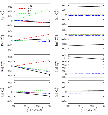
Figure 2: (Color online) One-loop contributions to the form factors C3AC^{A}_{3}, C4AC^{A}_{4}, C5AC^{A}_{5}, and C6AC^{A}_{6}. The pion-pole diagrams, which only contribute to C6AC^{A}_{6}, have not been included. The NN-NN, NN-Δ\Delta, Δ\Delta-NN, Δ\Delta-Δ\Delta labels denote the contributions of diagrams with nucleon-nucleon, nucleon-Delta, Delta-nucleon, Delta-Delta internal lines.

Before presenting the loop results we specify our regularization procedure due to the complications with the power counting mentioned in Section II.A. The loops are regularized in the M​S¯\overline{MS} scheme, subtracting in addition the real part of the contribution to the form factors at q2q^{2}=0. Since there is no counter terms linear in q2q^{2} at δ(2)\delta^{(2)}, this procedure guarantees to recover the power counting in all form factors.

We show in Fig. 2 the one-loop contributions to the form factors C3AC^{A}_{3}, C4AC^{A}_{4}, C5AC^{A}_{5}, and C6AC^{A}_{6} (except the pion-pole diagrams which only contribute to C6AC^{A}_{6}). One can see that only diagrams c, d (NN-NN) and g, h (Δ\Delta-NN) from Fig. 1 contribute to the imaginary part of the form factors, with NN-NN being dominant. One also finds that C4AC^{A}_{4} and C6AC^{A}_{6} receive relatively small corrections from the one-loop calculation, whereas C3AC^{A}_{3} gets a relatively large one coming from the Δ\Delta-Δ\Delta diagrams (diagrams i, j). This seemingly large q2q^{2} dependence, however, suffers from the uncertainty related to the π​Δ​Δ\pi\Delta\Delta coupling HAH_{A} because the Δ\Delta-Δ\Delta loop contribution is proportional to HA2H^{2}_{A}.

Refer to caption
Refer to caption
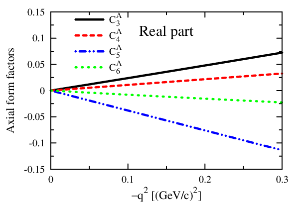
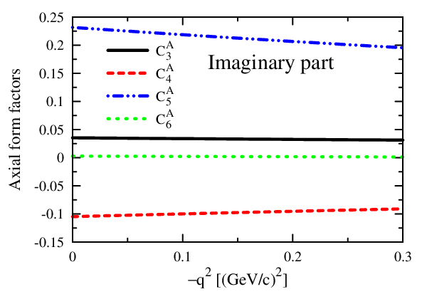
Figure 3: (Color online) One-loop contributions to the form factors C3AC^{A}_{3}, C4AC^{A}_{4}, C5AC^{A}_{5}, and C6AC^{A}_{6}. The pion-pole diagrams, which only contribute to C6AC^{A}_{6}, have not been included

In Fig. 3, the loop contributions from all diagrams to each form factor are added. Clearly, one can see that C5AC^{A}_{5} has the largest imaginary part; C4AC^{A}_{4} the second; next is the C3AC^{A}_{3}, and C6AC^{A}_{6} receives the smallest contribution.

Without the one-loop contributions, C6AC^{A}_{6} can be easily separated into a non-pole part and a pion-pole part, i.e.,

C6A=−g~π​N​Δ​MN2​23​[1q2−mπ2+16​rA2]C^{A}_{6}=-\tilde{g}_{\pi N\Delta}M^{2}_{N}\sqrt{\frac{2}{3}}\left[\frac{1}{q^{2}-m^{2}_{\pi}}+\frac{1}{6}r^{2}_{A}\right] (36)

with

g~π​N​Δ=hA2+d~3​Δ−f2​mπ2,\tilde{g}_{\pi N\Delta}=\frac{h_{A}}{2}+\tilde{d}_{3}\varDelta-f_{2}m^{2}_{\pi}, (37)
rA2=−6g~π​N​Δ​(f1+f2)≈6​dd​q2​log⁡(C5A)|q2=0.r_{A}^{2}=-\frac{6}{\tilde{g}_{\pi N\Delta}}(f_{1}+f_{2})\approx 6\frac{d}{dq^{2}}\log(C^{A}_{5})|_{q^{2}=0}. (38)

This is equivalent to the HBχ\chiPT result of Ref. [42]

rA2=−6Λx2​1gπ​N​Δ​[b3~+b8~2​ΛxMN+c2],r^{2}_{A}=-\frac{6}{\Lambda_{x}^{2}}\frac{1}{g_{\pi N\Delta}}\left[\frac{\tilde{b_{3}}+\tilde{b_{8}}}{2}\frac{\Lambda_{x}}{M_{N}}+c_{2}\right], (39)

with the correspondence g~π​N​Δ=gπ​N​Δ\tilde{g}_{\pi N\Delta}=g_{\pi N\Delta} and (f1+f2)=1Λx2​[b3~+b8~2​ΛxMN+c2](f_{1}+f_{2})=\frac{1}{\Lambda_{x}^{2}}\left[\frac{\tilde{b_{3}}+\tilde{b_{8}}}{2}\frac{\Lambda_{x}}{M_{N}}+c_{2}\right].

V Comparison with other approaches

V.1 Phenomenological fits

Bubble chamber neutrino data have been used to extract information about the axial N→ΔN\rightarrow\Delta form factors [9, 52, 53, 4]. However, there are some important limitations. First, the cross section is basically dominated by the C5AC_{5}^{A} form factor and shows very little sensitivity to C3,4,6AC_{3,4,6}^{A}. Second, the statistics is quite low and, furthermore, the two available data sets from BNL [9] and ANL [7] are clearly different. Finally, it is difficult to disentangle the Δ\Delta from other background pion production processes [3, 4]. Therefore, all these works make some additional assumptions. A set of them often found in the literature66 6 This choice originates from the analysis of Refs. [54, 1] of Adler’s results obtained using dispersion relations [55]. is: C3AC^{A}_{3}=0, C4A=−14​C5AC^{A}_{4}=-\frac{1}{4}C^{A}_{5}, and C6AC^{A}_{6} is related to C5AC^{A}_{5} through Eq. (35). In this way only C5AC^{A}_{5} is fitted to the experiment. As an example, we can take Kitagaki et al. [9] where it has the following functional form:

C5A​(q2)=C5A​(0)​[1−a5​q2b5−q2]​(1−q2MA2)−2C_{5}^{A}(q^{2})={{C_{5}^{A}(0)\left[1-{{a_{5}q^{2}}\over{b_{5}-q^{2}}}\right]}{\left(1-{{q^{2}}\over{M_{A}^{2}}}\right)^{-2}}} (40)

with C5A​(0)=1.2C_{5}^{A}(0)=1.2, a5=−1.21a_{5}=-1.21, b5=2b_{5}=2 GeV2, and MAM_{A} is fitted to data yielding MA=1.28−0.10+0.08M_{A}=1.28^{+0.08}_{-0.10} GeV. We will refer to this set of form factors as Kitagaki-Adler (KA) form factors.

As we have shown above, there are 5 independent parameters in the δ\delta expansion scheme up to chiral order 3: d~1\tilde{d}_{1}, d~2\tilde{d}_{2}, d~3\tilde{d}_{3}, f1f_{1} and f2f_{2}. We fix them in such a way that the real part of our form factors reproduces many of the features of the KA ones. To obtain C3A=0C^{A}_{3}=0, we set d~2=0\tilde{d}_{2}=0; therefore its contribution comes only from loop calculations which are of chiral order 3. Strictly speaking , Eq. (35) is not fulfilled at order δ(3)\delta^{(3)} but, if one neglects the small loop contributions, it can be satisfied by taking f1=0f_{1}=0. Correspondingly, the relation C4A​(0)=−14​C5A​(0)C^{A}_{4}(0)=-\frac{1}{4}C^{A}_{5}(0) fixes d~1\tilde{d}_{1}; C5A​(0)=1.2C^{A}_{5}(0)=1.2 fixes d~3\tilde{d}_{3}. The only LEC left, f2f_{2}, is then fixed to reproduce ∂C5A∂q2\frac{\partial C^{A}_{5}}{\partial q^{2}} at q2=0q^{2}=0.

Refer to caption
Figure 4: (Color online) Comparison with the Kitagaki-Adler form factors. The dark shadowed area indicates the uncertainty of MA=1.28−0.10+0.08M_{A}=1.28^{+0.08}_{-0.10} GeV as determined in Ref. [9]. The light shadowed area indicates the sensitivity of the results to the π​Δ​Δ\pi\Delta\Delta coupling HAH_{A}, which covers HA=(9/5)​gAH_{A}=(9/5)g_{A} to HA=gAH_{A}=g_{A}.

The results obtained this way are shown in Fig. 4, with the following parameter values d~1=−0.514\tilde{d}_{1}=-0.514 GeV-1, d~2=0\tilde{d}_{2}=0, d~3=0.153\tilde{d}_{3}=0.153 GeV-1, f1=0f_{1}=0, and f2=−2.184f_{2}=-2.184 GeV-2. One can clearly see that the calculated C5AC^{A}_{5} and C6AC^{A}_{6} are in good agreement with the KA form factors. On the other hand, the q2q^{2} dependence of C4AC^{A}_{4} is much weaker that the one assumed in KA, C4A=−C5A4C^{A}_{4}=-\frac{C^{A}_{5}}{4}, and we cannot accommodate their results at order δ(3)\delta^{(3)}. For C3AC^{A}_{3}, the q2q^{2} dependence is also very weak (compared to C5AC^{A}_{5}). In Fig. 4, the dark shadowed area indicates a modification of MAM_{A} within its uncertainties as given in Ref. [9]. As we mentioned above, the C3AC^{A}_{3} dependence on q2q^{2} is rather sensitive to the coupling constant HAH_{A}. This can be easily seen from the light shadowed area in the upper-left panel of Fig. 4, which covers the region of gA≤HA≤(9/5)​gAg_{A}\leq H_{A}\leq(9/5)g_{A}. The form factors, C4,5,6AC^{A}_{4,5,6}, on the other hand, are less sensitive to the value of HAH_{A}.

A word of caution is in place about the comparison of C3AC^{A}_{3} and C4AC^{A}_{4} with the KA form factors. In χ\chiPT, the leading order counter terms linear in q2q^{2} contributing to C3AC^{A}_{3} and C4AC^{A}_{4} appear at chiral order 4. A fair comparison with the phenomenological fits (particularly the q2q^{2} dependence) should, in principle, be done at order 4. However, the δ(3)\delta^{(3)} χ\chiPT results might give us a clue on the magnitude of the q2q^{2} dependence of C3AC^{A}_{3} and C4AC^{A}_{4}. Furthermore, if we believe in the phenomenological assumption, or the results of other approaches, the difference between the third order χ\chiPT results and the results of other approaches might help us estimate the value of the corresponding fourth order LEC. Indeed, the upper panels of Fig. 4 indicate that small δ(4)\delta^{(4)} corrections hi​q2h_{i}q^{2} with natural values for the LEC hih_{i} can reproduce the slope assumed for C3AC^{A}_{3} and C4AC^{A}_{4} by the KA ansatz.

We also notice that a recent analysis [4] obtained a smaller value for C5A​(0)C^{A}_{5}(0) by including non Δ\Delta contributions and fitting to the low invariant mass ANL data. In the present χ\chiPT study, we do have the higher-order contributions, d~3\tilde{d}_{3}, which could alter C5A​(0)C^{A}_{5}(0) within such a range; however, the same LEC appear in pion-nucleon scattering processes. A combined analysis is mandatory to determine whether one can accommodate the small C5A​(0)C^{A}_{5}(0) obtained in, for instance, Ref. [4]. This is left for future studies.

V.2 Quark models

There have been many studies of the N→ΔN\rightarrow\Delta axial transition form factors in various quark models, both relativistic and non-relativistic. For a brief review of quark model studies, we refer the readers to Refs. [10, 11]. Compared to dynamical model studies, a feature of most quark model calculations is that the obtained form factors are real due to time-reversal symmetry, while in dynamical models, like our χ\chiPT study, these form factors are in general complex due to the opening of the pion-nucleon channel.

Quark model results are in fact quite scattered. Taking, for instance, the models discussed in Ref. [11], we observed that the prediction of C5A​(0)C^{A}_{5}(0) runs from 0.81 to 1.53, C4A​(0)C^{A}_{4}(0) runs from −0.66-0.66 to 0.14 and C3A​(0)C^{A}_{3}(0) runs from 0 to 0.05. These models also obtain the non-pole part of C6AC^{A}_{6} whose value at q2=0q^{2}=0 ranges from −0.72-0.72 to 1.13. We could use these results to extract our constants although the large differences between them do not allow to reach solid conclusions about their values. From C5A​(0)C^{A}_{5}(0) one gets d~3\tilde{d}_{3}, and from its slope ∂C5A/∂q2\partial C^{A}_{5}/\partial q^{2} at q2=0q^{2}=0, (f1+f2)(f_{1}+f_{2}). This fixes the non-pole part of C6A​(0)C^{A}_{6}(0) (neglecting the one-loop corrections) since

C6A⁡(non−pole)​(0)≈23​MN2​(f1+f2),C^{A\mathrm{(non-pole)}}_{6}(0)\approx\sqrt{\frac{2}{3}}M^{2}_{N}(f_{1}+f_{2})\,, (41)

which is nothing but a direct consequence of PCAC. Using the quark model calculation of Ref. [11] for C5AC^{A}_{5} we obtain C6A⁡(non−pole)​(0)≈−2C^{A\mathrm{(non-pole)}}_{6}(0)\approx-2. This value is almost a factor three larger in magnitude than the one obtained directly from that model in spite of the fact that it implements PCAC at the quark level by introducing one- and two-body axial exchange currents.

Analogously, we can use quark model results for C3AC^{A}_{3} and C4AC^{A}_{4} at q2=0q^{2}=0 to obtain d~1\tilde{d}_{1} and d~2\tilde{d}_{2}. The smallness of C3A​(0)C^{A}_{3}(0) predicted by all calculations points towards a d~2\tilde{d}_{2} close to zero, in agreement with the phenomenological assumption. The situation is much more uncertain with d~1\tilde{d}_{1}, both in sign and magnitude. In Fig. 5, the q2q^{2} dependence of the real parts of C3AC^{A}_{3} and C4AC^{A}_{4} in our calculation, which at order δ(3)\delta^{(3)} is dictated by the loops, is compared to several quark models. As in the case of the KA form factors discussed above, we can expect from this comparison that next order terms linear in q2q^{2} with small (natural) values of the LEC are sufficient to eliminate the discrepancies in the low q2q^{2} behavior with any of these quark models.

Refer to caption
Refer to caption
Figure 5: (Color online) Comparison with the non relativistic Isgur-Karl and D-mixing quark model results of Ref. [10], and those of the chiral quark models of Refs. [11] and  [56].

V.3 Lattice QCD results

Recently, the N→ΔN\rightarrow\Delta axial transition form factors have been studied in lattice QCD  [13, 14]. Some major conclusions are (i) C3AC^{A}_{3} and C4AC^{A}_{4} are suppressed compared to C5AC^{A}_{5} and C6AC^{A}_{6}, and (ii) C5AC^{A}_{5} can be described by a dipole ansatz C5A​(0)/(1+Q2/MA2)2C^{A}_{5}(0)/(1+Q^{2}/M^{2}_{A})^{2} but with a smaller C5A​(0)C^{A}_{5}(0) and a larger MAM_{A} (≳1.5\gtrsim 1.5 GeV), compared to the Kitagaki-Adler form factors. These results should be taken with caution because of the still relatively large pion mass (≥350\geq 350 MeV) used in the study.

In principle, χ\chiPT is the perfect tool to extrapolate the lattice QCD results to the physical region. Meanwhile, one can also fix the unknown couplings to the lattice QCD results. Due to the regularization method we used and the fact that the lattice data points are still scarce, we will leave this subject to the future.

VI Summary and conclusions

We have studied the axial N→ΔN\rightarrow\Delta transition form factors up to one-loop order in relativistic baryon chiral perturbation theory with the δ\delta expansion scheme. The adopted Lagrangians including the Δ⁡(1232)\Delta(1232) are consistent, i.e., spin-3/2 gauge symmetric, which automatically decouples unphysical spin-1/2 fields. Consequently, our results do not depend on the specific value of the gauge-fixing parameter that is present in the most general spin-3/2 propagator, and avoid various problems related to inconsistent couplings.

The form factor C5AC^{A}_{5} exhibits the richest structure in our study. It receives contributions starting at chiral order 1, at which we find that C5A​(0)=23​hA2≈1.16C^{A}_{5}(0)=\sqrt{\frac{2}{3}}\frac{h_{A}}{2}\approx 1.16 for hA=2.85h_{A}=2.85. At higher orders, this value is modified by low energy constants that are unknown but which also appear in pion-nucleon scattering. At chiral order 3, this form factor gets q2q^{2} dependent contributions, some of them complex. Actually, we find that C5AC^{A}_{5} has the largest imaginary part among the four form factors. We also obtain that, up to chiral order 2, C6A=C5A​MN2mπ2−q2C^{A}_{6}=C^{A}_{5}\frac{M^{2}_{N}}{m^{2}_{\pi}-q^{2}}. At order 3, C6AC^{A}_{6} has a non-pole contribution whose value at q2=0q^{2}=0 is related to the slope of C5AC^{A}_{5} at q2=0q^{2}=0. Assuming natural values for the LEC, this non-pole part is small compared to the dominant pion-pole mechanism.

Both C3AC^{A}_{3} and C4AC^{A}_{4} start at chiral order 2 and get their q2q^{2} dependence at order 3 from the loops. For C3AC^{A}_{3}, we find a small q2q^{2} dependence, which is quite sensitive to the π​Δ​Δ\pi\Delta\Delta coupling constant, HAH_{A}. On the other hand, its imaginary part, coming mainly from the NN-NN internal diagram, is finite (∼0.03\sim 0.03 at q2=0q^{2}=0) and has a mild q2q^{2} dependence. This suggests that C3AC^{A}_{3} is small (compared to C4,5,6AC^{A}_{4,5,6}) but not necessarily zero. The C4AC^{A}_{4} dependence on q2q^{2} is also found to be rather mild at order δ(3)\delta^{(3)}.

We have compared our results with a phenomenological set of form factors used in the analysis of neutrino-induced pion production data and also with different quark model calculations. They could be used to extract the low energy constants but the scarcity of data and the large differences between quark model results make it difficult to come to solid conclusions. In the case of C3AC^{A}_{3} and specially C4AC^{A}_{4}, the comparison should, in principle, be done at order 4 where corresponding leading order counter terms linear in q2q^{2} appear. Nevertheless we can say that reasonable agreement with all these approaches can be obtained with natural values of the LEC.

Future experiments with electron and neutrino beams, combined with the analysis of pion-nucleon scattering data, can shed more light on these form factors. The extrapolation of lattice QCD results to the physical region should also be pursued.

VII Acknowledgments

We thank Mauro Napsuciale, Stefan Scherer, Wolfram Weise, and in particular Massimiliano Procura and Vladimir Pascalutsa for useful discussions. We are also grateful to Eliecer Hernandez for providing us with the results of several quark model calculations. L. S. Geng acknowledges financial support from the Ministerio de Educacion y Ciencia in the Program “Estancias de doctores y tecnologos extranjeros”. J. Martin Camalich acknowledges the same institution for a FPU fellowship. This work was partially supported by the MEC contract FIS2006-03438, the Generalitat Valenciana ACOMP07/302, and the EU Integrated Infrastructure Initiative Hadron Physics Project contract RII3-CT-2004-506078.

Note added in proof: After submitting this paper, a new preprint [57] appeared that studies the N→ΔN\rightarrow\Delta axial form factors up to one-loop order in HBChPT using the small scale expansion scheme. Within this framework, there is no q2q^{2} dependence coming from the loop-functions. This supports the smooth q2q^{2} dependences found in the present work. Namely, the q2q^{2} dependence of the loops in our relativistic framework is counted as of higher-order in HBChPT.

References

  • [1] C. H. Llewellyn Smith, Phys. Rept. 3, 261 (1972).
  • [2] G. L. Fogli and G. Nardulli, Nucl. Phys. B160, 116 (1979).
  • [3] T. Sato, D. Uno, and T. S. H. Lee, Phys. Rev. C67, 065201 (2003).
  • [4] E. Hernandez, J. Nieves, and M. Valverde, Phys. Rev. D76, 033005 (2007).
  • [5] L. Alvarez-Ruso, L. S. Geng, and M. J. Vicente Vacas, Phys. Rev. C76, 068501 (2007).
  • [6] S. J. Barish et al., Phys. Rev. D19, 2521 (1979).
  • [7] G. M. Radecky et al., Phys. Rev. D25, 1161 (1982).
  • [8] T. Kitagaki et al., Phys. Rev. D34, 2554 (1986).
  • [9] T. Kitagaki et al., Phys. Rev. D42, 1331 (1990).
  • [10] J. Liu, N. C. Mukhopadhyay, and L.-s. Zhang, Phys. Rev. C52, 1630 (1995).
  • [11] D. Barquilla-Cano, A. J. Buchmann, and E. Hernandez, Phys. Rev. C75, 065203 (2007).
  • [12] T. M. Aliev, K. Azizi, and A. Ozpineci, Nucl. Phys. A799, 105 (2008).
  • [13] C. Alexandrou, T. Leontiou, J. W. Negele, and A. Tsapalis, Phys. Rev. Lett. 98, 052003 (2007a).
  • [14] C. Alexandrou, G. Koutsou, T. Leontiou, J. W. Negele, and A. Tsapalis, Phys. Rev. D76, 094511 (2007b).
  • [15] S. P. Wells et al. (G0 Collaboration), JLAB experiment No. E97-104 (1997).
  • [16] N. C. Mukhopadhyay, M. J. Ramsey-Musolf, S. J. Pollock, J. Liu, and H. W. Hammer, Nucl. Phys. A633, 481 (1998).
  • [17] S.-L. Zhu, C. M. Maekawa, B. R. Holstein, and M. J. Ramsey-Musolf, Phys. Rev. Lett. 87, 201802 (2001).
  • [18] M. Hasegawa et al. (K2K), Phys. Rev. Lett. 95, 252301 (2005).
  • [19] J. L. Raaf (BooNE), Nucl. Phys. Proc. Suppl. 139, 47 (2005).
  • [20] M. O. Wascko (MiniBooNE), Nucl. Phys. Proc. Suppl. 159, 79 (2006).
  • [21] K. B. M. Mahn, Nucl. Phys. Proc. Suppl. 159, 237 (2006).
  • [22] D. Drakoulakos et al. (Minerva) (2004), eprint hep-ex/0405002.
  • [23] D. S. Ayres et al. (NOvA) (2004), eprint hep-ex/0503053.
  • [24] S. Weinberg, Physica A96, 327 (1979).
  • [25] J. Gasser and H. Leutwyler, Nucl. Phys. B250, 465 (1985).
  • [26] G. Ecker, Prog. Part. Nucl. Phys. 35, 1 (1995).
  • [27] S. Scherer, Adv. Nucl. Phys. 27, 277 (2003).
  • [28] J. Gasser, M. E. Sainio, and A. Svarc, Nucl. Phys. B307, 779 (1988).
  • [29] E. E. Jenkins and A. V. Manohar, Phys. Lett. B255, 558 (1991).
  • [30] V. Bernard, N. Kaiser, and U.-G. Meissner, Int. J. Mod. Phys. E4, 193 (1995).
  • [31] T. Becher and H. Leutwyler, Eur. Phys. J. C9, 643 (1999).
  • [32] J. Gegelia, G. Japaridze, and X. Q. Wang, J. Phys. G29, 2303 (2003).
  • [33] T. Fuchs, J. Gegelia, G. Japaridze, and S. Scherer, Phys. Rev. D68, 056005 (2003).
  • [34] T. R. Hemmert, B. R. Holstein, and J. Kambor, J. Phys. G24, 1831 (1998).
  • [35] V. Pascalutsa and D. R. Phillips, Phys. Rev. C68, 055205 (2003).
  • [36] V. Bernard, T. R. Hemmert, and U.-G. Meissner, Phys. Lett. B565, 137 (2003).
  • [37] C. Hacker, N. Wies, J. Gegelia, and S. Scherer, Phys. Rev. C72, 055203 (2005).
  • [38] G. C. Gellas, T. R. Hemmert, C. N. Ktorides, and G. I. Poulis, Phys. Rev. D60, 054022 (1999).
  • [39] T. A. Gail and T. R. Hemmert, Eur. Phys. J. A28, 91 (2006).
  • [40] V. Pascalutsa and M. Vanderhaeghen, Phys. Rev. Lett. 95, 232001 (2005).
  • [41] V. Pascalutsa and M. Vanderhaeghen, Phys. Rev. D73, 034003 (2006a).
  • [42] S.-L. Zhu and M. J. Ramsey-Musolf, Phys. Rev. D66, 076008 (2002).
  • [43] V. Pascalutsa, M. Vanderhaeghen, and S. N. Yang, Phys. Rept. 437, 125 (2007).
  • [44] N. Fettes and U. G. Meissner, Nucl. Phys. A679, 629 (2001).
  • [45] V. Pascalutsa, Phys. Lett. B503, 85 (2001).
  • [46] V. Pascalutsa and M. Vanderhaeghen, Phys. Lett. B636, 31 (2006b).
  • [47] P. A. Schreiner and F. Von Hippel, Nucl. Phys. B58, 333 (1973).
  • [48] J. A. M. Vermaseren (2000), eprint math-ph/0010025.
  • [49] R. Mertig, M. Bohm, and A. Denner, Comput. Phys. Commun. 64, 345 (1991).
  • [50] G. J. van Oldenborgh and J. A. M. Vermaseren, Z. Phys. C46, 425 (1990).
  • [51] T. Hahn and M. Perez-Victoria, Comput. Phys. Commun. 118, 153 (1999).
  • [52] L. Alvarez-Ruso, S. K. Singh, and M. J. Vicente Vacas, Phys. Rev. C59, 3386 (1999).
  • [53] O. Lalakulich and E. A. Paschos, Phys. Rev. D71, 074003 (2005).
  • [54] J. Bijtebier, Nucl. Phys. B21, 158 (1970).
  • [55] S. L. Adler, Ann. Phys. 50, 189 (1968).
  • [56] B. Golli, S. Sirca, L. Amoreira, and M. Fiolhais, Phys. Lett. B553, 51 (2003).
  • [57] M. Procura (2008), eprint arXiv: 0803.4291 [hep-ph].
  • [58] V. A. Smirnov (2006), Feynman Integral Calculus, Berlin, Germany: Springer.

VIII Appendix

VIII.1 Isospin transition matrices and antisymmetric Gamma matrix products

The isospin 1/2 to 3/2 and 3/2 to 3/2 transition matrices TaT^{a} and 𝒯a\mathcal{T}^{a} appearing in the N​ΔN\Delta and Δ​Δ\Delta\Delta Lagrangians are given by:

T1=16​(−30100−103),T^{1}=\frac{1}{\sqrt{6}}\left(\begin{array}[]{cccc}-\sqrt{3}&0&1&0\\ 0&-1&0&\sqrt{3}\end{array}\right), (42)
T2=−i6​(30100103),T^{2}=\frac{-i}{\sqrt{6}}\left(\begin{array}[]{cccc}\sqrt{3}&0&1&0\\ 0&1&0&\sqrt{3}\end{array}\right), (43)
T3=23​(01000010).T^{3}=\sqrt{\frac{2}{3}}\left(\begin{array}[]{cccc}0&1&0&0\\ 0&0&1&0\end{array}\right). (44)
𝒯1=23​(03/2003/20100103/2003/20),\mathcal{T}^{1}=\frac{2}{3}\left(\begin{array}[]{cccc}0&\sqrt{3}/2&0&0\\ \sqrt{3}/2&0&1&0\\ 0&1&0&\sqrt{3}/2\\ 0&0&\sqrt{3}/2&0\end{array}\right), (45)
𝒯2=2​i3​(0−3/2003/20−10010−3/2003/20),\mathcal{T}^{2}=\frac{2i}{3}\left(\begin{array}[]{cccc}0&-\sqrt{3}/2&0&0\\ \sqrt{3}/2&0&-1&0\\ 0&1&0&-\sqrt{3}/2\\ 0&0&\sqrt{3}/2&0\end{array}\right), (46)
𝒯3=(100001/30000−1/30000−1).\mathcal{T}^{3}=\left(\begin{array}[]{cccc}1&0&0&0\\ 0&1/3&0&0\\ 0&0&-1/3&0\\ 0&0&0&-1\end{array}\right). (47)

The totally antisymmetric Gamma matrix products appearing in the consistent N​ΔN\Delta and Δ​Δ\Delta\Delta Lagrangians are defined as:

γμ​ν=12​[γμ,γν],\gamma^{\mu\nu}=\frac{1}{2}[\gamma^{\mu},\gamma^{\nu}], (48)
γμ​ν​ρ=12​{γμ​ν,γρ}=−i​εμ​ν​ρ​σ​γσ​γ5,\gamma^{\mu\nu\rho}=\frac{1}{2}\{\gamma^{\mu\nu},\gamma^{\rho}\}=-i\varepsilon^{\mu\nu\rho\sigma}\gamma_{\sigma}\gamma_{5}, (49)
γμ​ν​ρ​σ=12​[γμ​ν​ρ,γσ]=i​εμ​ν​ρ​σ​γ5\gamma^{\mu\nu\rho\sigma}=\frac{1}{2}[\gamma^{\mu\nu\rho},\gamma^{\sigma}]=i\varepsilon^{\mu\nu\rho\sigma}\gamma_{5} (50)

with the following conventions: gμ​ν=diag⁡(1,−1,−1,−1)g^{\mu\nu}=\mathrm{diag}(1,-1,-1,-1), ε0,1,2,3=−ε0,1,2,3=1\varepsilon_{0,1,2,3}=-\varepsilon^{0,1,2,3}=1, γ5=i​γ0​γ1​γ2​γ3\gamma_{5}=i\gamma_{0}\gamma_{1}\gamma_{2}\gamma_{3}.

VIII.2 Loop functions

In the calculation of the loop diagrams, we have used the following dd-dimensional integrals in Minkowski space:

∫dd​k​kα1​…​kα2​n(ℳ2−k2)λ=i​πd/2​Γ⁡(λ−n+ϵ−2)2n​Γ​(λ)​(−1)n​gsα1​…​α2​n(ℳ2)λ−n+ϵ−2\int d^{d}k\frac{k^{\alpha_{1}}\ldots k^{\alpha_{2n}}}{(\mathcal{M}^{2}-k^{2})^{\lambda}}=i\pi^{d/2}\frac{\Gamma(\lambda-n+\epsilon-2)}{2^{n}\Gamma(\lambda)}\frac{(-1)^{n}g^{\alpha_{1}\ldots\alpha_{2n}}_{s}}{(\mathcal{M}^{2})^{\lambda-n+\epsilon-2}} (51)

with gsα1​…​α2​n=gα1​α2​…​gα2​n−1​α2​n+…g^{\alpha_{1}\ldots\alpha_{2n}}_{s}=g^{\alpha_{1}\alpha_{2}}\ldots g^{\alpha_{2n-1}\alpha_{2n}}+\ldots a combination symmetrical with respect to the permutation of any pair of indices (with (2​n−1)!!(2n-1)!! terms in the sum) [58].

The ℳ2\mathcal{M}^{2} that appear in the calculation of the NN-NN, NN-Δ\Delta, Δ\Delta-NN, and Δ\Delta-Δ\Delta internal diagrams are, respectively,

ℳN​N2=x​mπ2−x⁡(1−x−y)​MΔ2+(1−x−x​y)​MN2−y⁡(1−x−y)​q2−i​ϵ,\mathcal{M}_{NN}^{2}=x\,m_{\pi}^{2}-x(1-x-y)M_{\Delta}^{2}+(1-x-xy)M_{N}^{2}-y(1-x-y)q^{2}-i\epsilon, (52)
ℳN​Δ2=x​mπ2+(1−x)​(1−x−y)​MΔ2+y⁡(1−x)​MN2−y⁡(1−x−y)​q2−i​ϵ,\mathcal{M}_{N\Delta}^{2}=x\,m_{\pi}^{2}+(1-x)(1-x-y)M_{\Delta}^{2}+y(1-x)M_{N}^{2}-y(1-x-y)q^{2}-i\epsilon, (53)
ℳΔ​N2=x​mπ2+(x2+x​y−x+y)​MΔ2+(1−x−y−x​y)​MN2−y⁡(1−x−y)​q2−i​ϵ,\mathcal{M}_{\Delta N}^{2}=x\,m_{\pi}^{2}+(x^{2}+xy-x+y)M_{\Delta}^{2}+(1-x-y-xy)M_{N}^{2}-y(1-x-y)q^{2}-i\epsilon, (54)
ℳΔ​Δ2=x​mπ2+(1−2​x+x2+x​y)​MΔ2−x​y​MN2−y⁡(1−x−y)​q2−i​ϵ,\mathcal{M}_{\Delta\Delta}^{2}=x\,m_{\pi}^{2}+(1-2x+x^{2}+xy)M_{\Delta}^{2}-xyM_{N}^{2}-y(1-x-y)q^{2}-i\epsilon, (55)

where xx and yy are Feynman parameters.

VIII.3 Feynman parameterization integrals

We present below the loop integrals, diagrams (c), (e), (g) and (i) of Fig. 1, cast in the Feynman parameterization. We use the following notation: C~i(X​Y)\widetilde{C}_{i}^{(XY)} is the M​S¯\overline{MS}-regularized contribution of the loop to CiAC_{i}^{A} with XX and YY being the baryons in the internal line (in this order), ℳ¯X​Y2\bar{\mathcal{M}}^{2}_{XY}=ℳX​Y2/MΔ2\mathcal{M}^{2}_{XY}/M_{\Delta}^{2}, r=MN/MΔr=M_{N}/M_{\Delta}, μπ=mπ/MΔ\mu_{\pi}=m_{\pi}/M_{\Delta}, and Q¯2​n=Q2​n/MΔ2​n\bar{Q}^{2n}=Q^{2n}/M_{\Delta}^{2n} (with Q2=−q2Q^{2}=-q^{2}).

The couplings are contained in the constants 𝒞X​Y{\cal C}_{XY}:

𝒞N​N\displaystyle{\cal C}_{NN} =\displaystyle= 2​23​gA2​hA​MΔ2128​fπ2​π2;𝒞N​Δ=53​23​gA​hA​HA​MΔ2192​fπ2​π2;\displaystyle 2\,\sqrt{\frac{2}{3}}\;\frac{g_{A}^{2}h_{A}M_{\Delta}^{2}}{128f_{\pi}^{2}\pi^{2}}\;\;;\;\;{\cal C}_{N\Delta}=\frac{5}{3}\,\sqrt{\frac{2}{3}}\;\frac{g_{A}h_{A}H_{A}M_{\Delta}^{2}}{192f_{\pi}^{2}\pi^{2}}\;\;;
𝒞Δ​N\displaystyle{\cal C}_{\Delta N} =\displaystyle= 13​23​hA3​MΔ2192​fπ2​π2;𝒞Δ​Δ=109​23​hA​HA2​MΔ2576​fπ2​π2.\displaystyle\frac{1}{3}\,\sqrt{\frac{2}{3}}\;\frac{h_{A}^{3}M_{\Delta}^{2}}{192f_{\pi}^{2}\pi^{2}}\,\;\;;\;\;{\cal C}_{\Delta\Delta}=\frac{10}{9}\,\sqrt{\frac{2}{3}}\;\frac{h_{A}H_{A}^{2}M_{\Delta}^{2}}{576f_{\pi}^{2}\pi^{2}}\,.

Then, the expressions of the loop functions are:

C~3(N​N)\displaystyle\widetilde{C}_{3}^{(NN)} =\displaystyle= −𝒞N​N24r(14r+3)+r𝒞N​N∫01dx∫01−xdy{[y((−3y+x(y2+2y−1)+1)r3\displaystyle-\frac{{\cal C}_{NN}}{24}r(14r+3)+r\,{\cal C}_{NN}\,\int_{0}^{1}dx\int_{0}^{1-x}dy\Big\{\Big[y\left(\left(-3y+x\left(y^{2}+2y-1\right)+1\right)\right.r^{3}
+\displaystyle+ ((y−1)​x2+(y2−y−1)​x−3​y+2)​r2−x⁡(y+3)​(x+y−1)​r+x⁡(−x2−2​y​xCLOSE\displaystyle\left.\left((y-1)x^{2}+\left(y^{2}-y-1\right)x-3y+2\right)r^{2}-x(y+3)(x+y-1)r+x\left(-x^{2}-2yx\right.\right.
+\displaystyle+ x−y2+y)+Q¯2(x+y−1)((y−1)(x+y)+r(y2+2y−1)))]1ℳ¯N​N2\displaystyle\left.\left.x-y^{2}+y\right)+\bar{Q}^{2}(x+y-1)\left((y-1)(x+y)+r\left(y^{2}+2y-1\right)\right)\right)\Big]\frac{1}{\bar{\mathcal{M}}^{2}_{NN}}
−\displaystyle- [2y(2y−1)+x(4y−1)+r(4y2+5y−1)]log(ℳ¯N​N2)},\displaystyle\Big[2y(2y-1)+x(4y-1)+r\left(4y^{2}+5y-1\right)\Big]\log\left(\bar{\mathcal{M}}^{2}_{NN}\right)\Big\}\,,
C~4(N​N)\displaystyle\widetilde{C}_{4}^{(NN)} =\displaystyle= r2​𝒞N​N6−2r2𝒞N​N∫01dx∫01−xdyy{[(−3y+x(y2+y−2)+2)r2−2x(x\displaystyle\frac{r^{2}\,{\cal C}_{NN}}{6}-2\,r^{2}\,{\cal C}_{NN}\,\int_{0}^{1}dx\int_{0}^{1-x}dy\,y\,\Big\{\Big[\left(-3y+x\left(y^{2}+y-2\right)+2\right)r^{2}-2x(x
+\displaystyle+ y−1)r−y(x+y−1)((1−y)Q¯2+x)]1ℳ¯N​N2−2(2y−1)log(ℳ¯N​N2)},\displaystyle y-1)r-y(x+y-1)\left((1-y)\bar{Q}^{2}+x\right)\Big]\frac{1}{\bar{\mathcal{M}}^{2}_{NN}}-2(2y-1)\log\left(\bar{\mathcal{M}}_{NN}^{2}\right)\Big\}\,,
C~5(N​N)\displaystyle\widetilde{C}_{5}^{(NN)} =\displaystyle= −1−rrC~3(N​N)−1−r2−Q¯22​r2C~4(N​N)−2r𝒞N​N∫01dx∫01−xdy((1−r)y+r+x)×\displaystyle-\frac{1-r}{r}\widetilde{C}_{3}^{(NN)}-\frac{1-r^{2}-\bar{Q}^{2}}{2\,r^{2}}\widetilde{C}_{4}^{(NN)}-2\,r\,{\cal C}_{NN}\,\int_{0}^{1}dx\int_{0}^{1-x}dy\,((1-r)y+r+x)\times
×\displaystyle\times log⁡(ℳ¯N​N2),\displaystyle\log\left(\bar{\mathcal{M}}^{2}_{NN}\right)\,,
C~6(N​N)\displaystyle\widetilde{C}_{6}^{(NN)} =\displaystyle= r2​𝒞N​N6−2r2𝒞N​N∫01dx∫01−xdyy{[y((x(y−1)−2y+1)r2+2(x+y−1)r\displaystyle\frac{r^{2}\,{\cal C}_{NN}}{6}-2\,r^{2}\,{\cal C}_{NN}\,\int_{0}^{1}dx\int_{0}^{1-x}dy\,y\,\Big\{\Big[y((x(y-1)-2y+1)r^{2}+2(x+y-1)r
−\displaystyle- x(x+y−1)+Q¯2(y−1)(x+y−1))]1ℳ¯N​N2−2(2y−1)log(ℳ¯N​N2)}.\displaystyle x(x+y-1)+\bar{Q}^{2}(y-1)(x+y-1))\Big]\frac{1}{\bar{\mathcal{M}}^{2}_{NN}}-2(2y-1)\log\left(\bar{\mathcal{M}}^{2}_{NN}\right)\Big\}\,.
C~3(N​Δ)\displaystyle\widetilde{C}_{3}^{(N\Delta)} =\displaystyle= 𝒞N​Δ288r(−39μπ+2155r2+27Q¯2+96r−69)−r𝒞N​Δ∫01dx∫01−xdy×\displaystyle\frac{{\cal C}_{N\Delta}}{288}r\left(-39\mu_{\pi}{}^{2}+155r^{2}+27\bar{Q}^{2}+96r-69\right)-r\,{\cal C}_{N\Delta}\,\int_{0}^{1}dx\int_{0}^{1-x}dy\,\times
×\displaystyle\times {y[x(x(y−1)−2y+1)yr4+y(−2x2−3yx+x+1)r3+((1−2y)x3+(3−2y)yx2\displaystyle\Big\{y\Big[x(x(y-1)-2y+1)yr^{4}+y\left(-2x^{2}-3yx+x+1\right)r^{3}+\left((1-2y)x^{3}+(3-2y)yx^{2}\right.
+\displaystyle+ OPEN(y2−1)​x+y)​r2+x⁡(2​x2+5​y​x+3​y2−y−2)​r+x⁡(x+1)​(x2+(2​y−1)​xCLOSE\displaystyle\left.\left(y^{2}-1\right)x+y\right)r^{2}+x\left(2x^{2}+5yx+3y^{2}-y-2\right)r+x(x+1)\left(x^{2}+(2y-1)x\right.
+\displaystyle+ OPEN(y−1)​y)+Q¯4​(y−1)​y​(x2+(2​y−1)​x+(y−1)​y)+Q¯2​((1−2​y)​x3+(2​(y−1)​r2CLOSECLOSE\displaystyle\left.(y-1)y\right)+\bar{Q}^{4}(y-1)y\left(x^{2}+(2y-1)x+(y-1)y\right)+\bar{Q}^{2}\left((1-2y)x^{3}+\left(2(y-1)r^{2}\right.\right.
−\displaystyle- OPEN2​r−4​y+3)​y​x2+(2​(r2−1)​y3+(−5​r2−5​r+1)​y2+(2​r2+r+2)​y−1)​x\displaystyle\left.\left.2r-4y+3\right)yx^{2}+\left(2\left(r^{2}-1\right)y^{3}+\left(-5r^{2}-5r+1\right)y^{2}+\left(2r^{2}+r+2\right)y-1\right)x\right.
+\displaystyle+ y((y−2y2)r2+(−3y2+2y+1)r−(y−1)2))]1ℳ¯N​Δ2−[(4−33y)x2+(33(r2\displaystyle\left.y\left(\left(y-2y^{2}\right)r^{2}+\left(-3y^{2}+2y+1\right)r-(y-1)^{2}\right)\right)\Big]\frac{1}{\bar{\mathcal{M}}^{2}_{N\Delta}}-\Big[(4-33y)x^{2}+\left(33\left(r^{2}\right.\right.
+\displaystyle+ OPENOPENQ¯2−1)​y2−(21​r2+32​r+21​Q¯2−5)​y+4)​x+y⁡((13−32​y)​r2+(8−48​y)​r−16​yCLOSE\displaystyle\left.\left.\bar{Q}^{2}-1\right)y^{2}-\left(21r^{2}+32r+21\bar{Q}^{2}-5\right)y+4\right)x+y\left((13-32y)r^{2}+(8-48y)r-16y\right.
+\displaystyle+ Q¯2(33y2−38y+13)+8)]log⁡(ℳ¯N​Δ2)4+13(4y−1)ℳ¯N​Δ2​log⁡(ℳ¯N​Δ2)4},\displaystyle\left.\bar{Q}^{2}\left(33y^{2}-38y+13\right)+8\right)\Big]\frac{\log\left(\bar{\mathcal{M}}^{2}_{N\Delta}\right)}{4}+13(4y-1)\frac{\bar{\mathcal{M}}^{2}_{N\Delta}\,\log\left(\bar{\mathcal{M}}^{2}_{N\Delta}\right)}{4}\Big\}\,,
C~4(N​Δ)\displaystyle\widetilde{C}_{4}^{(N\Delta)} =\displaystyle= −r2​𝒞N​Δ240(−45μπ+227r2+33Q¯2−152r−55)+r2𝒞N​Δ∫01dx∫01−xdy×\displaystyle-\frac{r^{2}\,{\cal C}_{N\Delta}}{240}\left(-45\mu_{\pi}{}^{2}+27r^{2}+33\bar{Q}^{2}-152r-55\right)+r^{2}\,{\cal C}_{N\Delta}\,\int_{0}^{1}dx\int_{0}^{1-x}dy\,\times
×\displaystyle\times {y[(3x(x(y−1)−2y+1)yr4−y((y+3)x2+5yx−3)r3+((2−5y)x3+(9−5y)yx2\displaystyle\Big\{y\Big[(3x(x(y-1)-2y+1)yr^{4}-y\left((y+3)x^{2}+5yx-3\right)r^{3}+\left((2-5y)x^{3}+(9-5y)yx^{2}\right.
+\displaystyle+ OPEN(5​y2−y−2)​x+y)​r2+x⁡((y+4)​x2+y⁡(y+8)​x+5​y2−y−4)​r+3​Q¯4​(yCLOSE\displaystyle\left.\left(5y^{2}-y-2\right)x+y\right)r^{2}+x\left((y+4)x^{2}+y(y+8)x+5y^{2}-y-4\right)r+3\bar{Q}^{4}(y
−\displaystyle- OPEN1)​y​(x2+(2​y−1)​x+(y−1)​y)+x⁡(2​x3+4​y​x2+(2​y2+y−2)​x+(y−1)​y)\displaystyle 1)y\left(x^{2}+(2y-1)x+(y-1)y\right)+x\left(2x^{3}+4yx^{2}+\left(2y^{2}+y-2\right)x+(y-1)y\right)
−\displaystyle- Q¯2​((5​y−2)​x3+y⁡(−6​(y−1)​r2+(y+3)​r+10​y−7)​x2+((−6​r2+r+5)​y3CLOSECLOSE\displaystyle\bar{Q}^{2}\left((5y-2)x^{3}+y\left(-6(y-1)r^{2}+(y+3)r+10y-7\right)x^{2}+\left(\left(-6r^{2}+r+5\right)y^{3}\right.\right.
+\displaystyle+ OPEN(15​r2+7​r−4)​y2−3​(2​r2+1)​y+2)​x+y⁡(3​y​(2​y−1)​r2+(5​y2−2​y−3)​rCLOSE\displaystyle\left.\left.\left(15r^{2}+7r-4\right)y^{2}-3\left(2r^{2}+1\right)y+2\right)x+y\left(3y(2y-1)r^{2}+\left(5y^{2}-2y-3\right)r\right.\right.
+\displaystyle+ (y−1)2))]12​ℳ¯N​Δ2+[(19y−2)x2+((−24r2+5r−24Q¯2+19)y2+(15r2+14r\displaystyle\left.\left.(y-1)^{2}\right)\right)\Big]\frac{1}{2\bar{\mathcal{M}}^{2}_{N\Delta}}+\Big[(19y-2)x^{2}+\left(\left(-24r^{2}+5r-24\bar{Q}^{2}+19\right)y^{2}+\left(15r^{2}+14r\right.\right.
+\displaystyle+ 15Q¯2−5)y−2)x+y(3(8y−3)r2+4(5y+1)r+4y−3Q¯2(8y2−9y+3)−2)]×\displaystyle\left.\left.15\bar{Q}^{2}-5\right)y-2\right)x+y\left(3(8y-3)r^{2}+4(5y+1)r+4y-3\bar{Q}^{2}\left(8y^{2}-9y+3\right)-2\right)\Big]\times
×\displaystyle\times log⁡(ℳ¯N​Δ2)2+(4y−1)9​ℳ¯N​Δ2​log⁡(ℳ¯N​Δ2)2},\displaystyle\frac{\log\left(\bar{\mathcal{M}}^{2}_{N\Delta}\right)}{2}+(4y-1)\frac{9\bar{\mathcal{M}}^{2}_{N\Delta}\,\log\left(\bar{\mathcal{M}}^{2}_{N\Delta}\right)}{2}\Big\}\,,
C~5(N​Δ)\displaystyle\widetilde{C}_{5}^{(N\Delta)} =\displaystyle= −1−rrC~3(N​Δ)−1−r2−Q¯22​r2C~4(N​Δ)+𝒞N​Δ1440(5(−27Q¯2+9(43−3r)r+158)μπ2\displaystyle-\frac{1-r}{r}\,\widetilde{C}_{3}^{(N\Delta)}-\frac{1-r^{2}-\bar{Q}^{2}}{2\,r^{2}}\,\widetilde{C}_{4}^{(N\Delta)}+\frac{{\cal C}_{N\Delta}}{1440}\left(5\left(-27\bar{Q}^{2}+9(43-3r)r+158\right)\mu_{\pi}{}^{2}\right.
+\displaystyle+ OPEN99​Q¯4+5​Q¯2​(r⁡(36​r−191)−57)+r⁡(r⁡(r⁡(81​r+385)+135)+5175)+290)\displaystyle\left.99\bar{Q}^{4}+5\bar{Q}^{2}(r(36r-191)-57)+r(r(r(81r+385)+135)+5175)+290\right)
−\displaystyle- 𝒞N​Δ∫01dx∫01−xdy{[((r−1)2+Q¯2)y((y−1)y(x+y−1)(x+y)Q¯4((1\displaystyle{\cal C}_{N\Delta}\,\int_{0}^{1}dx\int_{0}^{1-x}dy\,\Big\{\Big[\left((r-1)^{2}+\bar{Q}^{2}\right)y\left((y-1)y(x+y-1)(x+y)\bar{Q}^{4}\left((1\right.\right.
−\displaystyle- OPEN2​y)​x3+(2​r​(r⁡(y−1)−1)−4​y+3)​y​x2+(y⁡((y⁡(2​y−5)+2)​r2−5​y​r+r−2​y2+yCLOSECLOSE\displaystyle\left.\left.2y)x^{3}+(2r(r(y-1)-1)-4y+3)yx^{2}+\left(y\left((y(2y-5)+2)r^{2}-5yr+r-2y^{2}+y\right.\right.\right.\right.
+\displaystyle+ 2)−1)x+y(−(r+1)(2r+1)y2+(r(r+2)+2)y+r−1))Q¯2+(r−1)(r+1)2×\displaystyle\left.\left.\left.\left.2\right)-1\right)x+y\left(-(r+1)(2r+1)y^{2}+(r(r+2)+2)y+r-1\right)\right)\bar{Q}^{2}+(r-1)(r+1)^{2}\times\right.
×\displaystyle\times (r⁡(x−2)−x−1)​x​y2+x⁡(r⁡(r+2)+x)​(x2−1)−(r+1)​(−x​r3−r2+2​(r−1)​x3CLOSE\displaystyle\left.(r(x-2)-x-1)xy^{2}+x(r(r+2)+x)\left(x^{2}-1\right)-(r+1)\left(-xr^{3}-r^{2}+2(r-1)x^{3}\right.\right.
+\displaystyle+ (r(r2+r−4)−1)x2+x)y)]34​ℳ¯N​Δ2−[x3+4r2x2+2rx2+6x2+6r2x−2rx−x\displaystyle\left.\left.\left(r\left(r^{2}+r-4\right)-1\right)x^{2}+x\right)y\right)\Big]\frac{3}{4\bar{\mathcal{M}}^{2}_{N\Delta}}-\Big[x^{3}+4r^{2}x^{2}+2rx^{2}+6x^{2}+6r^{2}x-2rx-x
−\displaystyle- 4​r2+(r−1)2​(r+1)​(24​r​(x−1)−23​x−12)​y2+8​r−(r−1)​(−9​r3+4​r2+2​rCLOSE\displaystyle 4r^{2}+(r-1)^{2}(r+1)(24r(x-1)-23x-12)y^{2}+8r-(r-1)\left(-9r^{3}+4r^{2}+2r\right.
+\displaystyle+ OPEN(25​r−22)​x2+3​(r⁡(r⁡(5​r+6)−5)+2)​x+6)​y+3​Q¯4​y​(y⁡(8​y−9)+x⁡(8​y−5)+3)\displaystyle\left.(25r-22)x^{2}+3(r(r(5r+6)-5)+2)x+6\right)y+3\bar{Q}^{4}y(y(8y-9)+x(8y-5)+3)
−\displaystyle- Q¯2((25y−4)x2+(y(2y+r(6r(5−8y)+47y+3)+13)−6)x+y(−3(y(8y−17)\displaystyle\bar{Q}^{2}\left((25y-4)x^{2}+(y(2y+r(6r(5-8y)+47y+3)+13)-6)x+y\left(-3(y(8y-17)\right.\right.
+\displaystyle+ 6)r2+(y(47y−8)+13)r+(41−23y)y−22)+4)]log⁡(ℳ¯N​Δ2)4−[4(x−8y+5)\displaystyle\left.\left.6)r^{2}+(y(47y-8)+13)r+(41-23y)y-22\right)+4\right)\Big]\frac{\log\left(\bar{\mathcal{M}}^{2}_{N\Delta}\right)}{4}-\Big[4(x-8y+5)
+\displaystyle+ 9Q¯2(1−4y)+r(9r(1−4y)+68y+7)]ℳ¯N​Δ2​log⁡(ℳ¯N​Δ2)4},\displaystyle 9\bar{Q}^{2}(1-4y)+r(9r(1-4y)+68y+7)\Big]\frac{\bar{\mathcal{M}}^{2}_{N\Delta}\,\log\left(\bar{\mathcal{M}}^{2}_{N\Delta}\right)}{4}\Big\}\,,
C~6(N​Δ)\displaystyle\widetilde{C}_{6}^{(N\Delta)} =\displaystyle= −r2​𝒞N​Δ360(199r+3)+r2𝒞N​Δ∫01dx∫01−xydy{y[((r−2)r+x)(x−1)2+(r2+r\displaystyle-\frac{r^{2}\,{\cal C}_{N\Delta}}{360}(199r+3)+r^{2}\,{\cal C}_{N\Delta}\,\int_{0}^{1}dx\int_{0}^{1-x}\,y\,dy\,\Big\{y\Big[((r-2)r+x)(x-1)^{2}+\left(r^{2}+r\right.
−\displaystyle- OPEN2)​(r−x)​y​(x−1)+(r−1)2​(r+1)​x​y2−Q¯2​(x+y−1)​(x⁡(y−1)−y⁡(r+(r−1)​yCLOSECLOSE\displaystyle\left.2\right)(r-x)y(x-1)+(r-1)^{2}(r+1)xy^{2}-\bar{Q}^{2}(x+y-1)(x(y-1)-y(r+(r-1)y
+\displaystyle+ 2)+1)]12​ℳ¯N​Δ2+[(x+y−1)(5y−2)−5ry(y+1)]log⁡(ℳ¯N​Δ2)2}.\displaystyle 2)+1)\Big]\frac{1}{2\bar{\mathcal{M}}^{2}_{N\Delta}}+\Big[(x+y-1)(5y-2)-5ry(y+1)\Big]\frac{\log\left(\bar{\mathcal{M}}^{2}_{N\Delta}\right)}{2}\Big\}\,.
C~3(Δ​N)\displaystyle\widetilde{C}_{3}^{(\Delta N)} =\displaystyle= r​𝒞Δ​N1440(5(73r+95)μπ+22Q¯2(11r+54)+r(r(345r+467)+175)+359)\displaystyle\frac{r\,{\cal C}_{\Delta N}}{1440}\left(5(73r+95)\mu_{\pi}{}^{2}+2\bar{Q}^{2}(11r+54)+r(r(345r+467)+175)+359\right)
+\displaystyle+ r𝒞Δ​N∫01dx∫01−xdy{[((r+1)2+Q¯2)y(x+y−1)(x(y−1)2r3−(y+x(y2\displaystyle r\,{\cal C}_{\Delta N}\,\int_{0}^{1}dx\int_{0}^{1-x}dy\,\Big\{\Big[\left((r+1)^{2}+\bar{Q}^{2}\right)y(x+y-1)\left(x(y-1)^{2}r^{3}-\left(y+x\left(y^{2}\right.\right.\right.
+\displaystyle+ OPENOPENx⁡(y−1))−1)​r2+(Q¯2​(x+y−1)​(y−1)2+y+x⁡(−y​x+x−(y−2)​y+1)CLOSE\displaystyle\left.\left.\left.x(y-1)\right)-1\right)r^{2}+\left(\bar{Q}^{2}(x+y-1)(y-1)^{2}+y+x(-yx+x-(y-2)y+1)\right.\right.
−\displaystyle- 1)r+(x+y−1)(x2+(−yQ¯2+Q¯2+y+1)x−Q¯2y2))]14​ℳ¯Δ​N2−[(2x(4y2\displaystyle\left.\left.1\right)r+(x+y-1)\left(x^{2}+\left(-y\bar{Q}^{2}+\bar{Q}^{2}+y+1\right)x-\bar{Q}^{2}y^{2}\right)\right)\Big]\frac{1}{4\bar{\mathcal{M}}^{2}_{\Delta N}}-\Big[\left(2x\left(4y^{2}\right.\right.
−\displaystyle- OPENOPEN6​y+1)+(y−1)​(y⁡(5​y−4)+1))​r3+(5​y3−(x+17)​y2+(9−2​x​(3​x+5))​yCLOSE\displaystyle\left.\left.6y+1\right)+(y-1)(y(5y-4)+1)\right)r^{3}+\left(5y^{3}-(x+17)y^{2}+(9-2x(3x+5))y\right.
+\displaystyle+ OPEN2​x2+x−1)​r2+((3−13​y)​x2+2​(2−9​y)​y​x+y⁡(12−y⁡(5​y+7)))​r+(x−5​yCLOSE\displaystyle\left.2x^{2}+x-1\right)r^{2}+\left((3-13y)x^{2}+2(2-9y)yx+y(12-y(5y+7))\right)r+(x-5y
+\displaystyle+ 1)(x+y)2−2(r+x−2y)+2Q¯2(x+y−1)((4r−3)y2−(6r+3x+2)y+r+x)]×\displaystyle 1)(x+y)^{2}-2(r+x-2y)+2\bar{Q}^{2}(x+y-1)\left((4r-3)y^{2}-(6r+3x+2)y+r+x\right)\Big]\times
×\displaystyle\times log⁡(ℳ¯Δ​N2)4−(x+r(2−3y)+y+1)ℳ¯Δ​N2log(ℳ¯Δ​N2)},\displaystyle\frac{\log\left(\bar{\mathcal{M}}^{2}_{\Delta N}\right)}{4}-(x+r(2-3y)+y+1)\bar{\mathcal{M}}^{2}_{\Delta N}\log\left(\bar{\mathcal{M}}^{2}_{\Delta N}\right)\Big\}\,,
C~4(Δ​N)\displaystyle\widetilde{C}_{4}^{(\Delta N)} =\displaystyle= −r2​𝒞Δ​N720(120μπ+28Q¯2+r(175r+107)+190)+r2𝒞Δ​N∫01dx∫01−xdy×\displaystyle-\frac{r^{2}\,{\cal C}_{\Delta N}}{720}\left(120\mu_{\pi}{}^{2}+8\bar{Q}^{2}+r(175r+107)+190\right)+r^{2}\,{\cal C}_{\Delta N}\,\int_{0}^{1}dx\int_{0}^{1-x}dy\times
×\displaystyle\times {[y(x+y−1)(−xy(x+y−1)r4+(y+x(x+(x+2)y−1)−1)r3+(x(2y2+4xy\displaystyle\Big\{\Big[y(x+y-1)\left(-xy(x+y-1)r^{4}+(y+x(x+(x+2)y-1)-1)r^{3}+\left(x\left(2y^{2}+4xy\right.\right.\right.
+\displaystyle+ (x−2)x−2)+Q¯2(y(−y2−4xy+y−2(x−2)x+1)−1))r2+(−y+Q¯2((x\displaystyle\left.\left.\left.(x-2)x-2\right)+\bar{Q}^{2}\left(y\left(-y^{2}-4xy+y-2(x-2)x+1\right)-1\right)\right)r^{2}+\left(-y+\bar{Q}^{2}\left((x\right.\right.\right.
+\displaystyle+ 2)y2+x(x+4)y−3y+(x−4)x+1)−x(2y+x(x+y+3))+1)r+x−Q¯4y(x\displaystyle\left.\left.\left.2)y^{2}+x(x+4)y-3y+(x-4)x+1\right)-x(2y+x(x+y+3))+1\right)r+x-\bar{Q}^{4}y(x\right.
+\displaystyle+ OPENy−1)​(x+2​y−2)−x⁡(y+(x+y)​(2​x+y))+Q¯2​(x3+(5​y−3)​x2+(y⁡(5​y−4)CLOSECLOSE\displaystyle\left.y-1)(x+2y-2)-x(y+(x+y)(2x+y))+\bar{Q}^{2}\left(x^{3}+(5y-3)x^{2}+(y(5y-4)\right.\right.
+\displaystyle+ 1)x+y(y2+y−2)))]12​ℳ¯Δ​N2−[x3+((17−6Q¯2)y−3)x2+(y(2Q¯2(9−11y)\displaystyle\left.\left.1)x+y\left(y^{2}+y-2\right)\right)\right)\Big]\frac{1}{2\bar{\mathcal{M}}^{2}_{\Delta N}}-\Big[x^{3}+\left(\left(17-6\bar{Q}^{2}\right)y-3\right)x^{2}+\left(y\left(2\bar{Q}^{2}(9-11y)\right.\right.
+\displaystyle+ OPENOPEN21​y−8)+1)​x+r⁡((5​x+8)​y2+x⁡(5​x+14)​y−7​y+(x−4)​x+1)+r2​(y⁡(−6​x2CLOSECLOSE\displaystyle\left.\left.21y-8\right)+1\right)x+r\left((5x+8)y^{2}+x(5x+14)y-7y+(x-4)x+1\right)+r^{2}\left(y\left(-6x^{2}\right.\right.
+\displaystyle+ 4(3−4y)x+(3−5y)y+3)−1)+y(5y(y+1)−4Q¯2(y(4y−7)+3)−6)]log⁡(ℳ¯Δ​N2)2\displaystyle\left.\left.4(3-4y)x+(3-5y)y+3\right)-1\right)+y\left(5y(y+1)-4\bar{Q}^{2}(y(4y-7)+3)-6\right)\Big]\frac{\log\left(\bar{\mathcal{M}}^{2}_{\Delta N}\right)}{2}
−\displaystyle- 2(x+6y−2)ℳ¯Δ​N2log(ℳ¯Δ​N2)},\displaystyle 2(x+6y-2)\bar{\mathcal{M}}^{2}_{\Delta N}\log\left(\bar{\mathcal{M}}^{2}_{\Delta N}\right)\Big\}\,,
C~5(Δ​N)\displaystyle\widetilde{C}_{5}^{(\Delta N)} =\displaystyle= −1−rrC~3(Δ​N)−1−r2−Q¯22​r2C~4(Δ​N)−𝒞Δ​N1440(5(5Q¯2+r(26r+63)+5)μπ+28Q¯4\displaystyle-\frac{1-r}{r}\,\widetilde{C}_{3}^{(\Delta N)}-\frac{1-r^{2}-\bar{Q}^{2}}{2\,r^{2}}\,\widetilde{C}_{4}^{(\Delta N)}-\frac{{\cal C}_{\Delta N}}{1440}\left(5\left(5\bar{Q}^{2}+r(26r+63)+5\right)\mu_{\pi}{}^{2}+8\bar{Q}^{4}\right.
+\displaystyle+ Q¯2(42r2+52r+15)+r(r(r(193r+289)+114)+223)+7)−𝒞Δ​N∫01dx∫01−xdy×\displaystyle\left.\bar{Q}^{2}\left(42r^{2}+52r+15\right)+r(r(r(193r+289)+114)+223)+7\right)-{\cal C}_{\Delta N}\,\int_{0}^{1}dx\int_{0}^{1-x}dy\times
×\displaystyle\times {[(y2−(x2+2)y+1)r4+(y+x(y2+(x−2)y+x+2)−1)r3+(x3−2Q¯2(x\displaystyle\Big\{\Big[\left(y^{2}-\left(x^{2}+2\right)y+1\right)r^{4}+\left(y+x\left(y^{2}+(x-2)y+x+2\right)-1\right)r^{3}+\left(x^{3}-2\bar{Q}^{2}(x\right.
−\displaystyle- OPENOPEN1)​y​x−(2​Q¯2​x+x+2)​y2+2​y)​r2−(x+y−1)​(x2−(Q¯2+(Q¯2−1)​y+1)​xCLOSE\displaystyle\left.1)yx-\left(2\bar{Q}^{2}x+x+2\right)y^{2}+2y\right)r^{2}-(x+y-1)\left(x^{2}-\left(\bar{Q}^{2}+\left(\bar{Q}^{2}-1\right)y+1\right)x\right.
−\displaystyle- Q¯2y2)r+(Q¯2+1)(x+y−1)((Q¯2+1)y+(x+y)(x−Q¯2y))]log⁡(ℳ¯Δ​N2)4\displaystyle\left.\bar{Q}^{2}y^{2}\right)r+\left(\bar{Q}^{2}+1\right)(x+y-1)\left(\left(\bar{Q}^{2}+1\right)y+(x+y)\left(x-\bar{Q}^{2}y\right)\right)\Big]\frac{\log\left(\bar{\mathcal{M}}^{2}_{\Delta N}\right)}{4}
+\displaystyle+ (x+r((r−1)x−y)+y+Q¯2(x+y−1)−1)ℳ¯Δ​N2log(ℳ¯Δ​N2)},\displaystyle\left(x+r((r-1)x-y)+y+\bar{Q}^{2}(x+y-1)-1\right)\bar{\mathcal{M}}^{2}_{\Delta N}\log\left(\bar{\mathcal{M}}^{2}_{\Delta N}\right)\Big\}\,,
C~6(Δ​N)\displaystyle\widetilde{C}_{6}^{(\Delta N)} =\displaystyle= −r2​𝒞Δ​N720(95μπ+216Q¯2+r(121r+91)+199)−r2𝒞Δ​N∫01dx∫01−xdy×\displaystyle-\frac{r^{2}\,\mathcal{C}_{\Delta N}}{720}\left(95\mu_{\pi}{}^{2}+16\bar{Q}^{2}+r(121r+91)+199\right)-r^{2}\,\mathcal{C}_{\Delta N}\,\int_{0}^{1}dx\int_{0}^{1-x}dy\times
×\displaystyle\times {[y(x+y−1)((y−1)(xy+y−1)r4+x((y−4)y+3)r3+(2(x2+x+y)\displaystyle\Big\{\Big[y(x+y-1)\left((y-1)(xy+y-1)r^{4}+x((y-4)y+3)r^{3}+\left(2\left(x^{2}+x+y\right)\right.\right.
−\displaystyle- OPENy⁡(4​x2+3​y​x+2​y)+Q¯2​(y−1)​(y2+2​x​y−1))​r2+(Q¯2​((y−1)2+x⁡(y−3))​(yCLOSECLOSE\displaystyle\left.\left.y\left(4x^{2}+3yx+2y\right)+\bar{Q}^{2}(y-1)\left(y^{2}+2xy-1\right)\right)r^{2}+\left(\bar{Q}^{2}\left((y-1)^{2}+x(y-3)\right)(y\right.\right.
−\displaystyle- OPENOPEN1)+y−x⁡(x⁡(y−5)+(y−4)​y+1)−1)​r+3​x3+x2​(Q¯2​(2−4​y)+5​y−1)\displaystyle\left.\left.1)+y-x(x(y-5)+(y-4)y+1)-1\right)r+3x^{3}+x^{2}\left(\bar{Q}^{2}(2-4y)+5y-1\right)\right.
+\displaystyle+ (y−1)​y​((y−1)​Q¯4−2​y​Q¯2+1)+x⁡(((Q¯2−6)​Q¯2+2)​y2−(Q¯2−6)​Q¯2​y+yCLOSE\displaystyle\left.(y-1)y\left((y-1)\bar{Q}^{4}-2y\bar{Q}^{2}+1\right)+x\left(\left(\left(\bar{Q}^{2}-6\right)\bar{Q}^{2}+2\right)y^{2}-\left(\bar{Q}^{2}-6\right)\bar{Q}^{2}y+y\right.\right.
−\displaystyle- Q¯−21))]12​ℳ¯Δ​N2+[(y((2x(3−5y)+y(3−5y)+3)r2+(x(18−5y)+(13−5y)y\displaystyle\bar{Q}\left.\left.{}^{2}-1\right)\right)\Big]\frac{1}{2\bar{\mathcal{M}}^{2}_{\Delta N}}+\Big[\left(y\left((2x(3-5y)+y(3-5y)+3)r^{2}+(x(18-5y)+(13-5y)y\right.\right.
−\displaystyle- OPENOPEN7)​r+10​(x+y)​(2​x+y)−6​(3​x+y)−2​Q¯2​(x+y−1)​(5​y−3))−(r+x)​(r+2​xCLOSE\displaystyle\left.\left.7)r+10(x+y)(2x+y)-6(3x+y)-2\bar{Q}^{2}(x+y-1)(5y-3)\right)-(r+x)(r+2x\right.
−\displaystyle- 1))]log⁡(ℳ¯Δ​N2)2+2(5y−1)ℳ¯Δ​N2log(ℳ¯Δ​N2)}.\displaystyle\left.1)\right)\Big]\frac{\log\left(\bar{\mathcal{M}}^{2}_{\Delta N}\right)}{2}+2(5y-1)\bar{\mathcal{M}}^{2}_{\Delta N}\log\left(\bar{\mathcal{M}}^{2}_{\Delta N}\right)\Big\}\,.
C~3(Δ​Δ)\displaystyle\widetilde{C}_{3}^{(\Delta\Delta)} =\displaystyle= r​𝒞Δ​Δ1440(6620μπ+4(368Q¯2+7(483−320r)r+22011)μπ+2182Q¯4+Q¯2(2520\displaystyle\frac{r\,{\cal C}_{\Delta\Delta}}{1440}\left(6620\mu_{\pi}{}^{4}+\left(368\bar{Q}^{2}+7(483-320r)r+22011\right)\mu_{\pi}{}^{2}+182\bar{Q}^{4}+\bar{Q}^{2}(2520\right.
−\displaystyle- r(274r+3))+r(r(r(648r−625)−7941)+3789)+32345)+r𝒞Δ​Δ∫01dx∫01−xdy×\displaystyle\left.r(274r+3))+r(r(r(648r-625)-7941)+3789)+32345\right)+r\,{\cal C}_{\Delta\Delta}\,\int_{0}^{1}dx\int_{0}^{1-x}dy\times
×\displaystyle\times {[((r+1)2+Q¯2)y(x+y−1)(x4+2(Q¯2+(r−1)r−(r2+Q¯2)y+y+1)x3\displaystyle\Big\{\Big[\left((r+1)^{2}+\bar{Q}^{2}\right)y(x+y-1)\left(x^{4}+2\left(\bar{Q}^{2}+(r-1)r-\left(r^{2}+\bar{Q}^{2}\right)y+y+1\right)x^{3}\right.
+\displaystyle+ ((y−2)​y​Q¯4+(2​(y−2)​y​r2+(2​y−1)​r−4​y2+2​y−1)​Q¯2−(r−2)​r2+(r2−1)2​y2CLOSE\displaystyle\left.\left((y-2)y\bar{Q}^{4}+\left(2(y-2)yr^{2}+(2y-1)r-4y^{2}+2y-1\right)\bar{Q}^{2}-(r-2)r^{2}+\left(r^{2}-1\right)^{2}y^{2}\right.\right.
−\displaystyle- OPEN2​r​((r−1)​r2+2)​y+2​(r+2​y−1))​x2+(2​Q¯4​y​(y−1)2+(r−1)​((2​(y−1)​y−1)​r2CLOSECLOSE\displaystyle\left.\left.2r\left((r-1)r^{2}+2\right)y+2(r+2y-1)\right)x^{2}+\left(2\bar{Q}^{4}y(y-1)^{2}+(r-1)\left((2(y-1)y-1)r^{2}\right.\right.\right.
−\displaystyle- OPEN(y+1)​r−2​y2+y+3)+Q¯2​(2​r2​y​(y−1)2+r⁡(4​(y−1)​y−1)+y⁡(3−2​y​(y+1))CLOSE\displaystyle\left.\left.\left.(y+1)r-2y^{2}+y+3\right)+\bar{Q}^{2}\left(2r^{2}y(y-1)^{2}+r(4(y-1)y-1)+y(3-2y(y+1))\right.\right.\right.
−\displaystyle- 3))x+Q¯2(y−1)y((Q¯2(y−1)−2)y+r(2y−1)))]14​ℳ¯Δ​Δ2−[(xy(x(18y−19)\displaystyle\left.\left.\left.3\right)\right)x+\bar{Q}^{2}(y-1)y\left(\left(\bar{Q}^{2}(y-1)-2\right)y+r(2y-1)\right)\right)\Big]\frac{1}{4\bar{\mathcal{M}}^{2}_{\Delta\Delta}}-\Big[\left(xy(x(18y-19)\right.
+\displaystyle+ OPEN4​(y⁡(3​y−7)+3))​r4+(10​(2​x+1)​y3+(x⁡(20​x−19)−12)​y2+2​(1−6​x)​x​y−6​yCLOSE\displaystyle\left.4(y(3y-7)+3))r^{4}+\left(10(2x+1)y^{3}+(x(20x-19)-12)y^{2}+2(1-6x)xy-6y\right.\right.
−\displaystyle- OPEN2​x​(x+2)+4)​r3+(2​(5−14​y)​x3+(4​(5−8​y)​y+6)​x2+(y⁡((7−4​y)​y+19)−20)​xCLOSE\displaystyle\left.\left.2x(x+2)+4\right)r^{3}+\left(2(5-14y)x^{3}+(4(5-8y)y+6)x^{2}+(y((7-4y)y+19)-20)x\right.\right.
−\displaystyle- OPEN11​y+5​y2​(2​y−3)+8)​r2−(10​(2​x+1)​y3+(40​x2+x−4)​y2+x⁡(4​x+1)​(5​x−4)​yCLOSE\displaystyle\left.\left.11y+5y^{2}(2y-3)+8\right)r^{2}-\left(10(2x+1)y^{3}+\left(40x^{2}+x-4\right)y^{2}+x(4x+1)(5x-4)y\right.\right.
−\displaystyle- OPEN18​y−2​x​((x−1)​x+6)+8)​r+10​x4+(7−10​y)​y2+23​y+x3​(12​y+7)−2​x2​(3​(yCLOSECLOSE\displaystyle\left.\left.18y-2x((x-1)x+6)+8\right)r+10x^{4}+(7-10y)y^{2}+23y+x^{3}(12y+7)-2x^{2}(3(y\right.
−\displaystyle- OPENOPEN3)​y+19)+Q¯4​y​(x+y−1)​(3​y​(6​y−5)+x⁡(18​y−19)+5)+x⁡(y⁡(−8​y2+y−27)CLOSE\displaystyle\left.3)y+19)+\bar{Q}^{4}y(x+y-1)(3y(6y-5)+x(18y-19)+5)+x\left(y\left(-8y^{2}+y-27\right)\right.\right.
+\displaystyle+ OPEN31)+Q¯2​(2​(5−14​y)​x3+(8​(1−6​y)​y+2)​x2+y⁡(77−6​y​(2​y+7))​x−26​x−39​yCLOSE\displaystyle\left.\left.31\right)+\bar{Q}^{2}\left(2(5-14y)x^{3}+(8(1-6y)y+2)x^{2}+y(77-6y(2y+7))x-26x-39y\right.\right.
+\displaystyle+ y2​(8​(y−5)​y+67)+r2​y​((36​y−38)​x2+4​(4​y​(3​y−5)+9)​x+(y−1)2​(12​y−5))\displaystyle\left.\left.y^{2}(8(y-5)y+67)+r^{2}y\left((36y-38)x^{2}+4(4y(3y-5)+9)x+(y-1)^{2}(12y-5)\right)\right.\right.
+\displaystyle+ r⁡(2​(2​y​(5​y−3)−1)​x2+(5​y−2)​(y⁡(8​y−5)+2)​x+(y−1)​y​(y⁡(20​y−9)+11)+4)\displaystyle\left.\left.r\left(2(2y(5y-3)-1)x^{2}+(5y-2)(y(8y-5)+2)x+(y-1)y(y(20y-9)+11)+4\right)\right.\right.
+\displaystyle+ 12)−12)]log⁡(ℳ¯Δ​Δ2)4−[(28x+66y+Q¯2(−88y2+76y+x(38−88y)−28)\displaystyle\left.\left.12\right)-12\right)\Big]\frac{\log\left(\bar{\mathcal{M}}^{2}_{\Delta\Delta}\right)}{4}-\Big[\left(28x+66y+\bar{Q}^{2}\left(-88y^{2}+76y+x(38-88y)-28\right)\right.
−\displaystyle- 2((5y(3y−5)+x(44y−19)+7)r2+(4x(5y−1)+2y(10y−9)+7)r−(39x−5y)×\displaystyle\left.2\left((5y(3y-5)+x(44y-19)+7)r^{2}+(4x(5y-1)+2y(10y-9)+7)r-(39x-5y)\right.\right.\times
×\displaystyle\times (x+y))−67)]ℳ¯Δ​Δ2​log⁡(ℳ¯Δ​Δ2)4−14ℳ¯Δ​Δ4log(ℳ¯Δ​Δ2)},\displaystyle\left.\left.(x+y)\right)-67\right)\Big]\frac{\bar{\mathcal{M}}^{2}_{\Delta\Delta}\log\left(\bar{\mathcal{M}}^{2}_{\Delta\Delta}\right)}{4}-14\,\bar{\mathcal{M}}^{4}_{\Delta\Delta}\log\left(\bar{\mathcal{M}}^{2}_{\Delta\Delta}\right)\Big\}\,,
C~4(Δ​Δ)\displaystyle\widetilde{C}_{4}^{(\Delta\Delta)} =\displaystyle= −r2​𝒞Δ​Δ720(2340μπ+43(72Q¯2+(269−130r)r+2261)μπ+260Q¯4+Q¯2(788−r(42r\displaystyle-\frac{r^{2}\,{\cal C}_{\Delta\Delta}}{720}\left(2340\mu_{\pi}{}^{4}+3\left(72\bar{Q}^{2}+(269-130r)r+2261\right)\mu_{\pi}{}^{2}+60\bar{Q}^{4}+\bar{Q}^{2}(788-r(42r\right.
+\displaystyle+ 23))+r(r(r(90r+43)−1288)+1289)+8988)−r2𝒞Δ​Δ∫01dx∫01−xdy×\displaystyle\left.23))+r(r(r(90r+43)-1288)+1289)+8988\right)-r^{2}\,{\cal C}_{\Delta\Delta}\,\int_{0}^{1}dx\int_{0}^{1-x}dy\times
×\displaystyle\times {[y(x+y−1)((5Q¯2+r(5r−2)−1)x4+((4−8y)Q¯4+(14y+2r(r(4−8y)+y)\displaystyle\Big\{\Big[y(x+y-1)\left(\left(5\bar{Q}^{2}+r(5r-2)-1\right)x^{4}+\left((4-8y)\bar{Q}^{4}+(14y+2r(r(4-8y)+y)\right.\right.
+\displaystyle+ OPENOPEN1)​Q¯2−(r+1)​(2​y+r⁡(2​r​(−5​y+r⁡(4​y−2)+2)−5)+3))​x3+(3​(y−1)​y​r6−y​r5CLOSE\displaystyle\left.\left.1)\bar{Q}^{2}-(r+1)(2y+r(2r(-5y+r(4y-2)+2)-5)+3)\right)x^{3}+\left(3(y-1)yr^{6}-yr^{5}\right.\right.
+\displaystyle+ (−7​y2+y+3)​r4+(3−6​y)​r3+(y⁡(5​y+9)−4)​r2+7​y​r+r+Q¯4​(r⁡(9​r​(y−1)−1)CLOSE\displaystyle\left.\left.\left(-7y^{2}+y+3\right)r^{4}+(3-6y)r^{3}+(y(5y+9)-4)r^{2}+7yr+r+\bar{Q}^{4}(r(9r(y-1)-1)\right.\right.
−\displaystyle- OPEN19​y+11)​y+3​Q¯6​(y−1)​y−y⁡(y+7)+Q¯2​(9​(y−1)​y​r4−2​y​r3+(2​(6−13​y)​y+3)​r2CLOSE\displaystyle\left.\left.19y+11)y+3\bar{Q}^{6}(y-1)y-y(y+7)+\bar{Q}^{2}\left(9(y-1)yr^{4}-2yr^{3}+(2(6-13y)y+3)r^{2}\right.\right.\right.
−\displaystyle- 6yr+r+y(13y+7)−7)−1)x2+(3y(y(2y−3)+1)Q¯6+(y(6(y(2y−3)+1)r2\displaystyle\left.\left.\left.6yr+r+y(13y+7)-7\right)-1\right)x^{2}+\left(3y(y(2y-3)+1)\bar{Q}^{6}+\left(y\left(6(y(2y-3)+1)r^{2}\right.\right.\right.\right.
+\displaystyle+ OPENOPEN2​(y2+y−2)​r+(5−14​y)​y+7)−4)​Q¯4+(2​(r+1)2​(r⁡(3​r−5)+2)​y3+(10CLOSECLOSE\displaystyle\left.\left.\left.\left.2\left(y^{2}+y-2\right)r+(5-14y)y+7\right)-4\right)\bar{Q}^{4}+\left(2(r+1)^{2}(r(3r-5)+2)y^{3}+(10\right.\right.\right.
−\displaystyle- OPENOPENr⁡(r⁡(r⁡(9​r−8)+3)+10))​y2+(r−1)​(3​r3−7​r2+r+8)​y−5​r2+r−3)​Q¯2+(r2CLOSE\displaystyle\left.\left.\left.r(r(r(9r-8)+3)+10))y^{2}+(r-1)\left(3r^{3}-7r^{2}+r+8\right)y-5r^{2}+r-3\right)\bar{Q}^{2}+\left(r^{2}\right.\right.\right.
−\displaystyle- 1)(6(y−1)yr3+(−4y2+y−1)r2+3(−2y2+y+1)r+4y2−1))x+Q¯2(y−1)×\displaystyle\left.\left.\left.1\right)\left(6(y-1)yr^{3}+\left(-4y^{2}+y-1\right)r^{2}+3\left(-2y^{2}+y+1\right)r+4y^{2}-1\right)\right)x+\bar{Q}^{2}(y-1)\times\right.
×\displaystyle\times y⁡(3​(y−1)​y​Q¯4+(3​(y−1)​y​r2+(2​y​(y+2)−3)​r−y⁡(3​y+5)+1)​Q¯2+4​y+r⁡(−6​yCLOSECLOSE\displaystyle\left.y\left(3(y-1)y\bar{Q}^{4}+\left(3(y-1)yr^{2}+(2y(y+2)-3)r-y(3y+5)+1\right)\bar{Q}^{2}+4y+r(-6y\right.\right.
+\displaystyle+ r(−4y+r(6y−3)−1)+1)+1))]12​ℳ¯Δ​Δ2−[(3xy(10y2+14xy−16y−9x+6)r4\displaystyle\left.\left.r(-4y+r(6y-3)-1)+1)+1\right)\right)\Big]\frac{1}{2\bar{\mathcal{M}}^{2}_{\Delta\Delta}}-\Big[\left(3xy\left(10y^{2}+14xy-16y-9x+6\right)r^{4}\right.
+\displaystyle+ y⁡(6​(x+5)​y2+(33−4​x)​x​y−42​y−4​x​(x+7)+12)​r3+(−2​(23​x+10)​y3−6​(19​x2CLOSECLOSE\displaystyle\left.y\left(6(x+5)y^{2}+(33-4x)xy-42y-4x(x+7)+12\right)r^{3}+\left(-2(23x+10)y^{3}-6\left(19x^{2}\right.\right.\right.
+\displaystyle+ OPENOPENx−3)​y2+x⁡(−68​x2+46​x+31)​y−12​y+2​x​(x⁡(7​x+5)−9)+4)​r2+(−6​(x+5)​y3CLOSE\displaystyle\left.\left.\left.x-3\right)y^{2}+x\left(-68x^{2}+46x+31\right)y-12y+2x(x(7x+5)-9)+4\right)r^{2}+\left(-6(x+5)y^{3}\right.\right.
+\displaystyle+ OPEN(x−1)​(10​x−33)​y2+(x⁡(x⁡(16​x−29)+28)−1)​y+4​x2+6​x−4)​r+4​(4​x+5)​y3\displaystyle\left.\left.(x-1)(10x-33)y^{2}+(x(x(16x-29)+28)-1)y+4x^{2}+6x-4\right)r+4(4x+5)y^{3}\right.
+\displaystyle+ (46​x2+44​x−17)​y2+2​(x−1)​x​(x⁡(7​x+9)−9)+x⁡(4​x​(11​x+7)−49)​y+13​y\displaystyle\left.\left(46x^{2}+44x-17\right)y^{2}+2(x-1)x(x(7x+9)-9)+x(4x(11x+7)-49)y+13y\right.
+\displaystyle+ 3Q¯4y(x+y−1)(y(14y−13)+x(14y−9)+3)+Q¯2(2(7−34y)x3+2(y(3(14y−9)r2\displaystyle\left.3\bar{Q}^{4}y(x+y-1)(y(14y-13)+x(14y-9)+3)+\bar{Q}^{2}\left(2(7-34y)x^{3}+2\left(y\left(3(14y-9)r^{2}\right.\right.\right.\right.
−\displaystyle- 2(y+1)r−82y+35)+2)x2+(y(6(y(19y−26)+9)r2+(y(14y+23)−20)r+4(11\displaystyle\left.\left.\left.\left.2(y+1)r-82y+35\right)+2\right)x^{2}+\left(y\left(6(y(19y-26)+9)r^{2}+(y(14y+23)-20)r+4(11\right.\right.\right.\right.
−\displaystyle- 31y)y+53)−26)x+y(3(y−1)(2y−1)(5y−3)r2+(y(y(18y+11)−40)+17)r\displaystyle\left.\left.\left.\left.31y)y+53\right)-26\right)x+y\left(3(y-1)(2y-1)(5y-3)r^{2}+(y(y(18y+11)-40)+17)r\right.\right.\right.
+\displaystyle+ y(57−4y(7y+3))−29)+8)−4)]log⁡(ℳ¯Δ​Δ2)2+[(−16x−62y+12Q¯2(y(13y−12)\displaystyle\left.\left.\left.y(57-4y(7y+3))-29\right)+8\right)-4\right)\Big]\frac{\log\left(\bar{\mathcal{M}}^{2}_{\Delta\Delta}\right)}{2}+\Big[\left(-16x-62y+12\bar{Q}^{2}(y(13y-12)\right.
+\displaystyle+ OPENx⁡(13​y−4)+3)+2​(3​(2​y​(5​y−6)+x⁡(26​y−8)+3)​r2−(10​y​x+x−(3​y+5)​(5​y−2))​rCLOSE\displaystyle\left.x(13y-4)+3)+2\left(3(2y(5y-6)+x(26y-8)+3)r^{2}-(10yx+x-(3y+5)(5y-2))r\right.\right.
−\displaystyle- (x+y)(53x+25y))+39)]ℳ¯Δ​Δ2​log⁡(ℳ¯Δ​Δ2)2−36ℳ¯Δ​Δ4log(ℳ¯Δ​Δ2)},\displaystyle\left.\left.(x+y)(53x+25y)\right)+39\right)\Big]\frac{\bar{\mathcal{M}}^{2}_{\Delta\Delta}\log\left(\bar{\mathcal{M}}^{2}_{\Delta\Delta}\right)}{2}-36\bar{\mathcal{M}}^{4}_{\Delta\Delta}\log\left(\bar{\mathcal{M}}^{2}_{\Delta\Delta}\right)\Big\}\,,
C~5(Δ​Δ)\displaystyle\widetilde{C}_{5}^{(\Delta\Delta)} =\displaystyle= −1−rrC~3(Δ​Δ)−1−r2−Q¯22​r2C~4(Δ​Δ)+𝒞Δ​Δ1440(20(117Q¯2+r(117r−272)+117)μπ4\displaystyle-\frac{1-r}{r}\,\widetilde{C}_{3}^{(\Delta\Delta)}-\frac{1-r^{2}-\bar{Q}^{2}}{2\,r^{2}}\,\widetilde{C}_{4}^{(\Delta\Delta)}+\frac{{\cal C}_{\Delta\Delta}}{1440}\left(20\left(117\bar{Q}^{2}+r(117r-272)+117\right)\mu_{\pi}{}^{4}\right.
+\displaystyle+ (216​Q¯4+(2​(370−87​r)​r+7263)​Q¯2+r⁡(r⁡(−390​r2+2012​r+3773)−15462)CLOSE\displaystyle\left.\left(216\bar{Q}^{4}+(2(370-87r)r+7263)\bar{Q}^{2}+r\left(r\left(-390r^{2}+2012r+3773\right)-15462\right)\right.\right.
+\displaystyle+ 7047)μπ+260Q¯6+Q¯4(r(18r−109)+930)+Q¯2(r(48r3−717r+37)+11013)\displaystyle\left.\left.7047\right)\mu_{\pi}{}^{2}+60\bar{Q}^{6}+\bar{Q}^{4}(r(18r-109)+930)+\bar{Q}^{2}\left(r\left(48r^{3}-717r+37\right)+11013\right)\right.
+\displaystyle+ r(r(r(r(r(90r−347)−803)+5067)+3238)−21462)+10143)+𝒞Δ​Δ∫01dx∫01−xdy×\displaystyle\left.r(r(r(r(r(90r-347)-803)+5067)+3238)-21462)+10143\right)+{\cal C}_{\Delta\Delta}\,\int_{0}^{1}dx\int_{0}^{1-x}dy\,\times
×\displaystyle\times {[(r4+2(Q¯2−1)r2+(Q¯2+1)2)y(x+y−1)(x4+(r2+Q¯2−2(r2+Q¯2−1)y+1)x3\displaystyle\Big\{\Big[\left(r^{4}+2\left(\bar{Q}^{2}-1\right)r^{2}+\left(\bar{Q}^{2}+1\right)^{2}\right)y(x+y-1)\left(x^{4}+\left(r^{2}+\bar{Q}^{2}-2\left(r^{2}+\bar{Q}^{2}-1\right)y+1\right)x^{3}\right.
+\displaystyle+ ((y−1)​y​r4+(−2​y2+2​Q¯2​(y−1)​y+1)​r2−2​y​r+r+y⁡(Q¯2​(Q¯2​(y−1)−4​y+2)+y+3)CLOSE\displaystyle\left.\left((y-1)yr^{4}+\left(-2y^{2}+2\bar{Q}^{2}(y-1)y+1\right)r^{2}-2yr+r+y\left(\bar{Q}^{2}\left(\bar{Q}^{2}(y-1)-4y+2\right)+y+3\right)\right.\right.
−\displaystyle- OPEN1)​x2+(y⁡(y⁡(2​y−3)+1)​Q¯4+(y⁡((y⁡(2​y−3)+1)​r2+2​(y−1)​r−y⁡(2​y+1)+2)−1)​Q¯2CLOSE\displaystyle 1\left.\left.\right)x^{2}+\left(y(y(2y-3)+1)\bar{Q}^{4}+\left(y\left((y(2y-3)+1)r^{2}+2(y-1)r-y(2y+1)+2\right)-1\right)\bar{Q}^{2}\right.\right.
+\displaystyle+ OPEN(r−1)​((r+1)​(2​r​(y−1)−2​y+1)​y+1))​x+Q¯2​(y−1)​y​((Q¯2​(y−1)−2)​y+r⁡(2​yCLOSECLOSE\displaystyle\left.\left.(r-1)((r+1)(2r(y-1)-2y+1)y+1)\right)x+\bar{Q}^{2}(y-1)y\left(\left(\bar{Q}^{2}(y-1)-2\right)y+r(2y\right.\right.
−\displaystyle- 1)))]34​ℳ¯Δ​Δ2−[(11x3r4+8x2r4−9xr4−6x3r3+20xr3−4r3+10x4r2+9x3r2−12x2r2\displaystyle\left.\left.1)\right)\right)\Big]\frac{3}{4\bar{\mathcal{M}}^{2}_{\Delta\Delta}}-\Big[\left(11x^{3}r^{4}+8x^{2}r^{4}-9xr^{4}-6x^{3}r^{3}+20xr^{3}-4r^{3}+10x^{4}r^{2}+9x^{3}r^{2}-12x^{2}r^{2}\right.
−\displaystyle- x​r2+4​r2−10​x4​r−4​x3​r+32​x2​r−12​x​r+4​r+10​x4+10​x3+2​(r−1)3​(r+1)2​((15​rCLOSECLOSE\displaystyle\left.xr^{2}+4r^{2}-10x^{4}r-4x^{3}r+32x^{2}r-12xr+4r+10x^{4}+10x^{3}+2(r-1)^{3}(r+1)^{2}((15r\right.
+\displaystyle+ OPENOPEN16)​x+15)​y3−18​x2+(r−1)2​(r+1)​(6​x​(7​x−8)​r3+(30​x2+x−42)​r2+3​(−20​x2+xCLOSECLOSE\displaystyle\left.16)x+15)y^{3}-18x^{2}+(r-1)^{2}(r+1)\left(6x(7x-8)r^{3}+\left(30x^{2}+x-42\right)r^{2}+3\left(-20x^{2}+x\right.\right.\right.
−\displaystyle- 4)r−54x2+4x+31)y2+2x−(r−1)(9x(3x−2)r5+2(x(10x+9)−6)r4+(x(x(52x\displaystyle\left.\left.\left.4\right)r-54x^{2}+4x+31\right)y^{2}+2x-(r-1)\left(9x(3x-2)r^{5}+2(x(10x+9)-6)r^{4}+(x(x(52x\right.\right.
−\displaystyle- 31)+7)−6)r3+(x(30x2−9x−8)+9)r2+(x(−30x2+9x+20)+6)r+4(11−3x)x2\displaystyle\left.\left.31)+7)-6)r^{3}+\left(x\left(30x^{2}-9x-8\right)+9\right)r^{2}+\left(x\left(-30x^{2}+9x+20\right)+6\right)r+4(11-3x)x^{2}\right.\right.
+\displaystyle+ x+3)y+3Q¯6y(x+y−1)(y(14y−13)+x(14y−9)+3)+Q¯4((11−52y)x3+(y(−30y\displaystyle\left.\left.x+3\right)y+3\bar{Q}^{6}y(x+y-1)(y(14y-13)+x(14y-9)+3)+\bar{Q}^{4}\left((11-52y)x^{3}+(y(-30y\right.\right.
+\displaystyle+ OPENOPENr⁡(−12​y+9​r​(14​y−9)+7)−7)+2)​x2+(y⁡(6​(11​y​(3​y−4)+15)​r2+((71−24​y)​y−38)​rCLOSECLOSE\displaystyle\left.\left.r(-12y+9r(14y-9)+7)-7)+2)x^{2}+\left(y\left(6(11y(3y-4)+15)r^{2}+((71-24y)y-38)r\right.\right.\right.\right.
+\displaystyle+ OPENOPEN(y−1)​(96​y−113))−17)​x+y⁡(18​(y−1)​(r−2​r​y)2+y⁡(y⁡(74​y−191)+147)+2​r​(11CLOSECLOSE\displaystyle\left.\left.\left.\left.(y-1)(96y-113)\right)-17\right)x+y\left(18(y-1)(r-2ry)^{2}+y(y(74y-191)+147)+2r(11\right.\right.\right.
−\displaystyle- 2y(y(3y−16)+17))−34)+4)+Q¯2(3y(3(14y−9)x2+4(y(12y−17)+6)x+(y−1)(2y\displaystyle\left.\left.\left.2y(y(3y-16)+17))-34\right)+4\right)+\bar{Q}^{2}\left(3y\left(3(14y-9)x^{2}+4(y(12y-17)+6)x+(y-1)(2y\right.\right.\right.
−\displaystyle- OPENOPEN1)​(5​y−3))​r4+2​y​((7−12​y)​x2+((60−11​y)​y−37)​x+y⁡(y⁡(y+39)−54)+17)​r3+(2​(11CLOSECLOSE\displaystyle\left.\left.\left.1)(5y-3)\right)r^{4}+2y\left((7-12y)x^{2}+((60-11y)y-37)x+y(y(y+39)-54)+17\right)r^{3}+\left(2(11\right.\right.\right.
−\displaystyle- OPEN52​y)​x3+2​((22−81​y)​y+5)​x2−(y⁡(y⁡(120​y+23)−76)+26)​x+y⁡(y⁡((33−62​y)​y+21)CLOSE\displaystyle\left.\left.\left.52y)x^{3}+2((22-81y)y+5)x^{2}-(y(y(120y+23)-76)+26)x+y(y((33-62y)y+21)\right.\right.\right.
−\displaystyle- 14)+4)r2+((22y−6)x3+(42y2−34y+2)x2+(y(2y(9y+32)−79)+26)x−(y−1)×\displaystyle\left.\left.\left.14)+4\right)r^{2}+\left((22y-6)x^{3}+\left(42y^{2}-34y+2\right)x^{2}+(y(2y(9y+32)-79)+26)x-(y-1)\times\right.\right.\right.
×\displaystyle\times OPEN(y⁡(2​(y−45)​y+51)−12))​r+(x+y−1)​(32​y3−4​(13​x+27)​y2−x⁡(74​x+41)​y+22​yCLOSE\displaystyle\left.\left.\left.(y(2(y-45)y+51)-12)\right)r+(x+y-1)\left(32y^{3}-4(13x+27)y^{2}-x(74x+41)y+22y\right.\right.\right.
+\displaystyle+ x(2x+5)(5x+3)))−4)]log⁡(ℳ¯Δ​Δ2)4−[(48xr4−18r4−26xr3+38r3+86x2r2+36xr2\displaystyle\left.\left.\left.x(2x+5)(5x+3)\right)\right)-4\right)\Big]\frac{\log\left(\bar{\mathcal{M}}^{2}_{\Delta\Delta}\right)}{4}-\Big[\left(48xr^{4}-18r^{4}-26xr^{3}+38r^{3}+86x^{2}r^{2}+36xr^{2}\right.
−\displaystyle- 21​r2−82​x2​r−16​x​r+65​r+86​x2−10​(r−1)2​(r+1)​(6​r+7)​y2+38​x−2​(r−1)​(8​xCLOSE\displaystyle\left.21r^{2}-82x^{2}r-16xr+65r+86x^{2}-10(r-1)^{2}(r+1)(6r+7)y^{2}+38x-2(r-1)(8x\right.
+\displaystyle+ OPENr⁡(−28​x+r⁡(32​x+6​r​(13​x−6)+3)+6)+67)​y−12​Q¯4​(y⁡(13​y−12)+x⁡(13​y−4)+3)\displaystyle\left.r(-28x+r(32x+6r(13x-6)+3)+6)+67)y-12\bar{Q}^{4}(y(13y-12)+x(13y-4)+3)\right.
+\displaystyle+ Q¯2​(−6​(9​(1−2​y)2+4​x​(13​y−4))​r2+2​(46​y2−66​y+x⁡(46​y−13)+22)​r−226​y2CLOSE\displaystyle\left.\bar{Q}^{2}\left(-6\left(9(1-2y)^{2}+4x(13y-4)\right)r^{2}+2\left(46y^{2}-66y+x(46y-13)+22\right)r-226y^{2}\right.\right.
+\displaystyle+ 86x(x+1)−140xy+278y−75)−39)]ℳ¯Δ​Δ2​log⁡(ℳ¯Δ​Δ2)4−2(9Q¯2+r(9r−8)+9)×\displaystyle\left.\left.86x(x+1)-140xy+278y-75\right)-39\right)\Big]\frac{\bar{\mathcal{M}}^{2}_{\Delta\Delta}\log\left(\bar{\mathcal{M}}^{2}_{\Delta\Delta}\right)}{4}-2\left(9\bar{Q}^{2}+r(9r-8)+9\right)\times
×\displaystyle\times ℳ¯Δ​Δ4log(ℳ¯Δ​Δ2)},\displaystyle\bar{\mathcal{M}}^{4}_{\Delta\Delta}\log\left(\bar{\mathcal{M}}^{2}_{\Delta\Delta}\right)\Big\}\,,
C~6(Δ​Δ)\displaystyle\widetilde{C}_{6}^{(\Delta\Delta)} =\displaystyle= −r2​𝒞Δ​Δ720(5(36r+85)μπ+22(2Q¯2(8r+23)−3r(r(34r+65)−93)−839))\displaystyle-\frac{r^{2}\,{\cal C}_{\Delta\Delta}}{720}\left(5(36r+85)\mu_{\pi}{}^{2}+2\left(2\bar{Q}^{2}(8r+23)-3r(r(34r+65)-93)-839\right)\right)
+\displaystyle+ r2𝒞Δ​Δ∫01dx∫01−xdy{[y(1−x−y)(6x4+2(2(r2+r+Q¯2+1)−(5Q¯2+(r\displaystyle r^{2}\,{\cal C}_{\Delta\Delta}\,\int_{0}^{1}dx\int_{0}^{1-x}dy\,\Big\{\Big[y(1-x-y)\left(6x^{4}+2\left(2\left(r^{2}+r+\bar{Q}^{2}+1\right)-\left(5\bar{Q}^{2}+(r\right.\right.\right.
−\displaystyle- 1)(5r+7))y)x3+(2(2Q¯4+(r(4r+3)−11)Q¯2+(r−1)2(r+1)(2r+5))y2\displaystyle\left.\left.\left.1)(5r+7)\right)y\right)x^{3}+\left(2\left(2\bar{Q}^{4}+(r(4r+3)-11)\bar{Q}^{2}+(r-1)^{2}(r+1)(2r+5)\right)y^{2}\right.\right.
+\displaystyle+ (−3​Q¯4+(9−2​r​(3​r+4))​Q¯2−(r−1)​(r+3)​(r⁡(3​r+2)+4))​y+2​(Q¯2​(r+1)CLOSE\displaystyle\left.\left.\left(-3\bar{Q}^{4}+(9-2r(3r+4))\bar{Q}^{2}-(r-1)(r+3)(r(3r+2)+4)\right)y+2\left(\bar{Q}^{2}(r+1)\right.\right.\right.
+\displaystyle+ r(r(r+2)+2)−2))x2−((r(y−1)−4y+3)y(2y−1)Q¯4+(−9y+2(y(y(2y−3)\displaystyle\left.\left.\left.r(r(r+2)+2)-2\right)\right)x^{2}-\left((r(y-1)-4y+3)y(2y-1)\bar{Q}^{4}+\left(-9y+2\left(y(y(2y-3)\right.\right.\right.\right.
+\displaystyle+ 1)r3+y((6−5y)y−2)r2+(y(−4y2+2y+3)−1)r+y2(7y+1))+2)Q¯2\displaystyle\left.\left.\left.\left.1)r^{3}+y((6-5y)y-2)r^{2}+\left(y\left(-4y^{2}+2y+3\right)-1\right)r+y^{2}(7y+1)\right)+2\right)\bar{Q}^{2}\right.\right.
+\displaystyle+ (r−1)​(2​(r2−1)2​y3−(r−1)​(r+1)​(3​r2+r+8)​y2+(r⁡(r3+10​r+7)−6)​yCLOSE\displaystyle\left.\left.(r-1)\left(2\left(r^{2}-1\right)^{2}y^{3}-(r-1)(r+1)\left(3r^{2}+r+8\right)y^{2}+\left(r\left(r^{3}+10r+7\right)-6\right)y\right.\right.\right.
−\displaystyle- OPENOPEN2​(r2+r+1)))​x−(y−1)​y​(((2​r​(y−1)−4​y+3)​y−1)​Q¯4+(r⁡(y−1)−y)​(rCLOSECLOSE\displaystyle\left.\left.\left.2\left(r^{2}+r+1\right)\right)\right)x-(y-1)y\left(((2r(y-1)-4y+3)y-1)\bar{Q}^{4}+(r(y-1)-y)\left(r\right.\right.\right.
+\displaystyle+ 2(r2−1)y−9)Q¯2+(r−1)2(r+1)))]12​ℳ¯Δ​Δ2−[((56y−4)x3+(−2(22Q¯2+r(22r\displaystyle\left.\left.\left.2\left(r^{2}-1\right)y-9\right)\bar{Q}^{2}+(r-1)^{2}(r+1)\right)\right)\Big]\frac{1}{2\bar{\mathcal{M}}^{2}_{\Delta\Delta}}-\Big[\left((56y-4)x^{3}+\left(-2\left(22\bar{Q}^{2}+r(22r\right.\right.\right.
+\displaystyle+ 17)−62)y2+(20Q¯2+4r(5r+8)−31)y−2(r+1))x2+2((11Q¯2(r−4)\displaystyle\left.\left.\left.17)-62\right)y^{2}+\left(20\bar{Q}^{2}+4r(5r+8)-31\right)y-2(r+1)\right)x^{2}+2\left(\left(11\bar{Q}^{2}(r-4)\right.\right.\right.
+\displaystyle+ OPEN(r−1)​(r⁡(11​r−17)−40))​y3+(Q¯2​(47−13​r)+r⁡((30−13​r)​r+11)+2)​y2+(Q¯2​(3​rCLOSECLOSE\displaystyle\left.\left.\left.(r-1)(r(11r-17)-40)\right)y^{3}+\left(\bar{Q}^{2}(47-13r)+r((30-13r)r+11)+2\right)y^{2}+\left(\bar{Q}^{2}(3r\right.\right.\right.
−\displaystyle- 14)+r(r(3r−10)+5)−9)y−r+1)x+y(12(r−1)2(r+1)y3−(r−1)(r(24r\displaystyle\left.\left.\left.14)+r(r(3r-10)+5)-9\right)y-r+1\right)x+y\left(12(r-1)^{2}(r+1)y^{3}-(r-1)(r(24r\right.\right.
+\displaystyle+ OPENOPEN5)+31)​y2+r⁡(4​r​(4​r−3)+59)​y−32​y+r⁡((3−4​r)​r−21)+2​Q¯2​(y⁡((37−22​y)​y−22)CLOSE\displaystyle\left.\left.5)+31)y^{2}+r(4r(4r-3)+59)y-32y+r((3-4r)r-21)+2\bar{Q}^{2}(y((37-22y)y-22)\right.\right.
+\displaystyle+ (y−1)(y(11y−10)+2)+5)+1))]log⁡(ℳ¯Δ​Δ2)2+(7x+32y−50y(x+y)+r(y(25y\displaystyle\left.\left.(y-1)(y(11y-10)+2)+5)+1\right)\right)\Big]\frac{\log\left(\bar{\mathcal{M}}^{2}_{\Delta\Delta}\right)}{2}+(7x+32y-50y(x+y)+r(y(25y
−\displaystyle- 21)+2)−4)ℳ¯Δ​Δ2log(ℳ¯Δ​Δ2)}.\displaystyle 21)+2)-4)\bar{\mathcal{M}}^{2}_{\Delta\Delta}\log\left(\bar{\mathcal{M}}^{2}_{\Delta\Delta}\right)\Big\}.