Phase space patterns of quantum transport on ordered and disordered networks
Abstract
In this paper, we consider the quantum-mechanical phase space patterns on ordered and disordered networks. For ordered networks in which each node is connected to its nearest neighbors ( on either side), the phase space quasi-probability of Wigner function shows various patterns. In the long time limit, on even-numbered networks, we find an asymmetric quasi-probability between the node and its opposite node. This asymmetry depends on the network parameters and specific phase space positions. For disordered networks in which each edge is rewired with probability , the phase space displays regional localization on the initial node.
pacs
05.60.Gg, 03.67.-a, 05.40.-aI InTRoduction
Quantum walk (QW), which is a generalization of the classical random walk, has attracted a great deal of attention from the scientific community. The continuous interest in the study of quantum-mechanical transport process can be partly attributed to its broad applications in the field of quantum information and computation [1, 2, 3, 4]. In recent years, two types of quantum walks exist in the literature: the discrete-time quantum coined walks and continuous-time quantum walks [5, 6]. Both discrete-time quantum coined walks and continuous-time quantum walks have been argued to give an algorithmic speedup with respect to their classical counterparts [7].
In classical physics, the dynamical behavior of a system is described by phase space variables, such as position and momentum. A plot of position and momentum variables as a function of time shows the phase diagram of classical transport process. In contrast to the classical transport, the quantum-mechanical transport happens in the Hilbert space [8]. Such transport process needs to be formulated in phase space as a unified picture of the classical transport. This can be done by the widely used Wigner function, which transforms the wave function of a quantum mechanical state into a function in the position-momentum space analogously defined in the classical phase space [9]. It is shown in Ref. [10] that integrating the Wigner function along the lines in phase space is a positive value of probability and gives the correct marginal distributions. However, the negativity of Wigner function provides an indication of non-classical behavior.
The phase space method (Wigner function) provides a very useful tool for the study of quantum states in the field of statistical mechanics, quantum chemistry, molecular dynamics, scattering theory, quantum optics, etc [11, 12, 13, 14, 15, 16, 17]. There are various approaches available to generalize the Wigner function for quantum systems with a finite-dimensional space of states [18]. In Ref. [9], Wootters have introduced a discrete version of the Wigner function that has all the desired properties only when is a prime number. The phase space defined by Wootters is an grid ( is prime) and a Cartesian product of such spaces corresponding to prime factors of in the most general case [19]. Notably, a more general discrete Wigner function defined for a system with arbitrary values of has been introduced by Hannay and Berry in the studies of semiclassical properties of classically chaotic systems [20]. This version of Wigner function is used in several contexts and recently applied to analyze the phase-space representation of quantum computers and algorithms [19, 21, 22]. In this case, the phase space is constructed as a grid of points where the state is represented in a redundant manner (only of them are independent) [19]. Recently, Mülken et al propose a version of discrete phase space of Wigner function, which is defined for continuous-time quantum walks (CTQWs) on a one-dimensional discrete network with periodic boundary conditions [10]. This kind of discrete Wigner function recovers the correct marginal distributions when it is added over the horizonal and vertical lines. However, it is not positive when added over the general lines [19] in phase space. This is an unique feature differs from the usual Wigner function, which is positive when added over any lines [22].
Here, we use the version of discrete phase space of Wigner function proposed by Mülken [10]. In Ref. [10], Mülken et al formulate CTQWs in phase space on a network of size whose nodes are enumerated as . The Wigner function has the form of a Fourier transform as follows [10],
| (1) |
Where is the density operator of a pure state, and denote the phase space coordinate of positions. The summation over in the interval [) can be carried out in any consecutive values. Considering an initial exciton begins at node , the time evolution of the associated state is given by . Suppose and are the th eigenvalue and eigenstate of the Hamiltonian of Laplace matrix, the time independent Schrödinger equation is , where spans the whole accessible Hilbert space and forms an orthonormal complete basis set, i.e., , . Inserting the complete set condition of the eigenstates into the time evolution equation, we get,
| (2) |
The density operator of the system is . Substituting the above Equation into the Wigner function, we have,
| (3) |
In this paper, we use the above Equation to consider phase space patterns of CTQWs on ordered and disordered networks. For ordered networks, the topology organizes in a very regular manner, i.e., each node of the network is connected to its nearest neighbors ( on either side). For disordered networks, we employ the famous WS model [23], which triggers a surge of research of small-world networks in the field of complex networks [24, 25, 26, 27, 28]. In the WS model [23], each connection of the regular networks is rewired with probability . Tuning the rewiring probability interpolates the network topology between order () and disorder (or random with ). The intermediate value corresponds to the small-world region [23].
The paper is organized as follows. In Sec. II, we consider the phase space patterns on ordered networks which correspond to the WS model with rewiring probability . In Sec. III, we consider the phase space patterns on disordered networks. Conclusions and discussions are given in Sec. IV.
II Phase space patterns on ordered networks
In this section, we consider the quantum-mechanical phase space on one-dimension regular networks of nodes in which each node is connected to its nearest neighbors ( on either side). This generalized regular network has broad applications in various coupled dynamical systems, including biological oscillators [29], Josephson junction arrays [30], neural networks [31], synchronization [32], small-world networks [33] and many other self-organizing systems. We compute the phase space distribution on such general network with periodic boundary conditions in the framework of Bloch ansatz [34], which is commonly used in solid state physics.
II.1 Bloch ansatz and Wigner function
The Hamiltonian (H) of the system for CTQWs is related to the Laplace matrix (A) of the connected networks as . Here, for the sake of simplicity, we assume the transmission rate for all the connections to be equal. The nondiagonal elements equal to if nodes and are connected and otherwise. The diagonal elements equal to the number of total links connected to node , i.e., equals to the degree of node . Therefore, the Laplace matrix of ordered networks takes the following form,
| (4) |
The Hamiltonian acting on the state can be written as
| (5) |
The above Equation is the discrete version of the Hamiltonian for a free particle moving on the network. Using the approach of Bloch function [34] in solid state physics, the time independent Schrödinger equation reads
| (6) |
The Bloch states can be expanded as a linear combination of the states localized at node [34],
| (7) |
Substituting Eqs. (5) and (7) into Eq. (6), we obtain the eigenvalues (or energy) of the system,
| (8) |
The periodic boundary condition for the network requires that the projection of on the state equals to that on the state , thus with integer and . Replacing by the Bloch states in Eq. (3), we can get the Wigner function as follows,
| (9) |
The summation over can be written as , where takes value if equals to (or mod N) and otherwise. Thus the Wigner function can be simplified as,
| (10) |
Substituting the expression of eigenvalues of Eq. (8) into the above equation, we obtain discrete Wigner function of CTQWs on one-dimension ordered networks.
II.2 Time evolution of the Wigner function
We consider the time evolution of quantum-mechanical phase space according to Eq. (10). Figure 1 shows a contour plot of the Wigner function on ordered networks of size with different values of at different times. At very small time scales, the Wigner function is localized on the stripe at the initial node and its opposite node. As time increases, the Wigner function spreads over the whole network. On short time scales, the Wigner function has a very regular structure until the wave fronts between the initial node and opposite node start to interferes with each other. Interestingly, the phase space structure is more complex on highly connected networks compared to that on the cycle network (), and the nodes are populated more quickly on highly connected networks.
In Fig. 2, we plot the Wigner function of CTQWs on networks of size . The phase space structure is quite similar to that on even-numbered networks. We note that the phase space pictures provide us more information of the underlying dynamics than the transition probabilities. The phase space patterns alternate with time frequently. At long time scales, the phase space becomes irregular and we find that the structure of phase space has more regularities on even-numbered networks than that on odd-numbered networks with the same value of and . This indicates the higher topological symmetry of even-numbered networks.
It is worth noting that the pattern of Wigner function is symmetrical about the axis for . As increases, such behavior disappears and displays central symmetry at the phase space center . At the initial time , on even-numbered networks (or odd-numbered networks), the patterns of Wigner function are the same for different values of . This can be concluded from Eq. (10). For the case of even , equals to for arbitrary . At the opposite node , equals to for even and for odd . The nonzero values of the Wigner function at continue to show up at later times. The analysis for odd is similar but the patterns are different. The Wigner function equals to for and otherwise. The nonzero of at the opposite node ( Evens) is a natural consequence of the periodic boundary conditions of the regular networks [10]. At later times, involves contribution from all the eigenstates and the nodes connected to the excitation node get populated, resulting the semicircle-like areas on highly connected networks. We remark that during all the time the patterns show central symmetry at , to this end, we conjecture that central symmetry is an intrinsical feature of the phase space patterns.
II.3 Long time averages
The Wigner function of a specific position () fluctuates around a constant value, thus it is interesting to study the long time averaged phase space patterns. The time limiting Wigner function is defined as,
| (11) |
For the ordered networks, the limiting Wigner function can be simplified as,
| (12) |
This expression shortens the numerical time of computation considerably compared to Eq. (11). Therefore, we consider the long time averaged phase space structure according to Eq. (12).
For the cycle network () in which each node is only connected to its two nearest neighbors, the limiting phase space has a simple structure. For even-numbered networks (), the limiting phase space structure is
| (13) |
If the network size is an odd number, we can also obtain the limiting Wigner function according to Eq. (12), which is summarized as,
| (14) |
which confirms the results in Ref. [35].
For other values of , the limiting phase space distributions can also be calculated in the same way, but such process is complicated for large value of because of the nontrivial degeneracy distribution of the eigenvalues. Here, we report the numerical results of phase space patterns on highly connected networks according to Eq. (12).
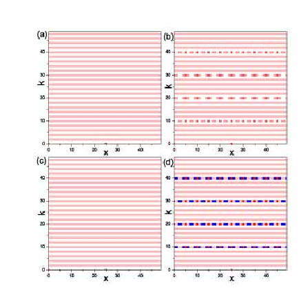
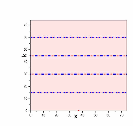
Fig. 3 shows the phase space patterns on networks of with different values of . We note that the phase space structure of is the same as the phase space structure of . After a careful examination, we find that and have the same degeneracy distributions of the eigenvalues. This explains the same phase space patterns of and . For and , there are some significant stripes in the phase space. Such nontrivial stripes reflect the topological symmetry of the considered networks. On the contrary, the phase space patterns on networks of with , and are the same as the structure with , which is described in Eq. (14). One may conjecture that the phase space patterns do not alter when increasing the connectivity on odd-numbered networks. But this is not true for some particular value of network size . For instance, on a network of and , we find significant stripes at some phase space positions (See Fig. 4).
The patterns of in Fig. 3 are the same for odd and some even . However, for some particular values of and even , the patterns are quite different (See the stripes at and in Fig. 3(b) and (d)). According to Eq. (12), depends on the degeneracy of the eigenstates, i.e., the Kronecker symbol . For , equals to for all the values of , thus the sum in Eq. (12) contains exponential terms, which results in for and otherwise. When is odd, holds for all the values of . For some values of even , equals to when and , this leads to ( arbitrary ). However, for some other values of even , does not vanish and is oscillatory on the horizontal lines located at and . The oscillating strip is caused by the interference between the positive strip and the mirror image. This is similar to the case of decoherence of quantum walks in phase space [13], in which there are interference fringes in lines between the two position eigenstates, and all the vertical lines have their corresponding oscillatory counterparts originated from the boundary conditions [13].
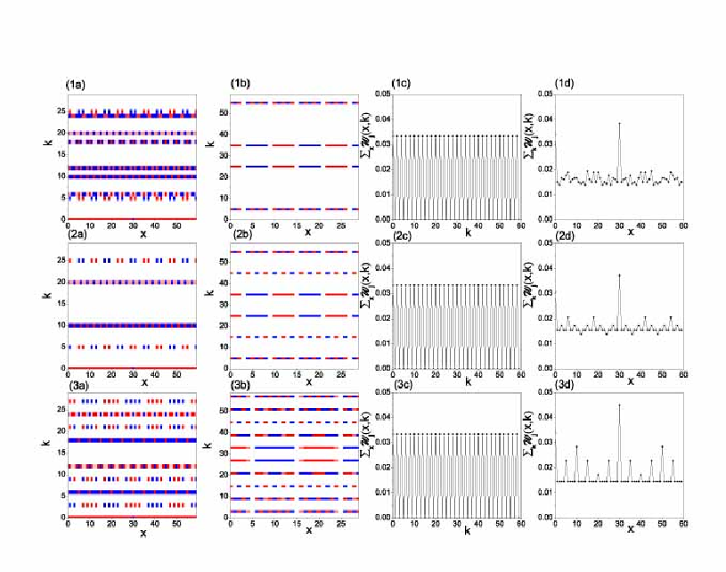
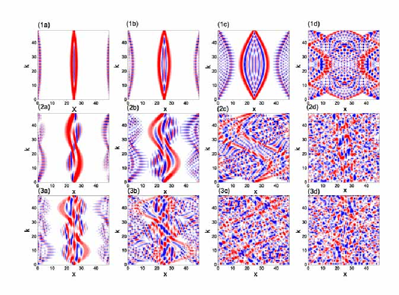
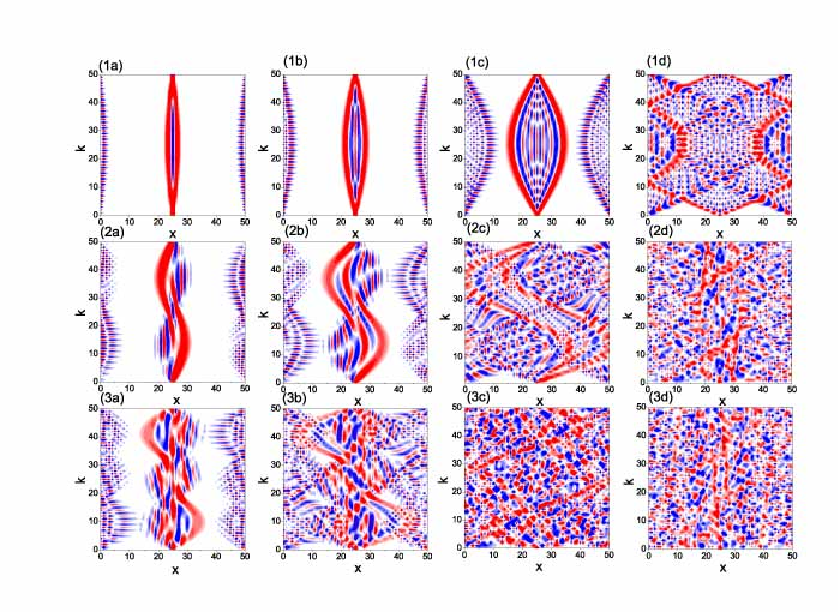
In Fig. 3, we find a symmetric structure of the phase space distributions in both the and directions. That is to say, equals to () for all the values of ; equals to () for all the values of . Such symmetric phase space structure exists on some even-numbered networks. However, for some even-numbered networks with certain values of , this is not true. For instance, on networks of size with , and , the Wigner function differs from () for some values of and also differs from () for some values of . Such asymmetry depends on the specific phase space positions . In Ref. [35], the authors find an asymmetry of transition probabilities for the starting node and its mirror node on two-dimensional networks, their definition of mirror node is based on geometry symmetry of the network. In this paper, we define the mirror node of a given node to be its opposite node, i.e., (or in the longitudinal direction). We study symmetric and asymmetric structure of the phase space on the and direction separately. The asymmetric phase space is particularly characterized by the difference between and () in the direction, and difference between and () in the direction. Therefore, we use the quantities and to detect the asymmetry of the phase space. Columns (a) and (b) of Fig. 5 show these two quantities in the phase space. The nonwhite blocks in the plot indicate asymmetric phase space positions. From the figure we find that the asymmetric structure in the phase space is very complex. The phase space positions in which asymmetry occurs is dependant on the precise values of network parameters and , as well as the specific phase space positions.
It is interesting to note that, in Figs. 1 and 3, has more identical values than in the phase space plane. and display central symmetry and mirror symmetry respectively. This suggests that the limiting Wigner function has higher symmetry in the structure compared to the instantaneous Wigner function .
II.4 Marginal distributions
Summing the Wigner function along lines in phase space gives the marginal distributions. Of course, such a process loses the detailed information of the phase space. Here, we consider marginal distributions of the long time averaged Wigner function summing over the direction and direction respectively. Summing over all recovers the time limiting transition probabilities, i.e.,
| (15) |
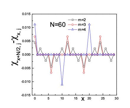
Columns (c) and (d) of Fig. 5 show the marginal distributions of the sum and . We find that the marginal distributions obtained by summing over for , and are the same (See column (c) in Fig. 5). equals to for even and for odd . In contrast, the marginal distributions for different values of are quite different (See column (d) in Fig. 5). Interestingly, there is a large probability to be still or again at the initial node () and at the opposite node (). In analogous to the analysis of the phase space asymmetry, we consider asymmetry of the limiting transition probability. We find that differs from () for some particular values of on networks with certain values of and . Fig. 6 shows the quantity for all the values of in the range . The nonzero values in the plot indicate asymmetric transition probabilities at the corresponding nodes.
As shown in Ref. [36], the asymmetries of transition probabilities originate from different contribution of eigenvalues to . It turns out that there are more contribution to in the asymmetric cases than in the symmetric cases [36]. The argumentation for our case is similar. Although all the eigenvalues can be analytically obtained, a complete analysis of all possible differences of eigenvalues requires extensive work and is clearly beyond the scope of this paper.
III phase space patterns on disordered networks
In this section, we study the phase space patterns on networks in the presence of two kinds of disorder: static disorder and topological disorder. We import static disorder by adding a perturbed Hamiltonian to the original Hamiltonian as done in Ref. [37]. This assumption do not create new connections or remove the existing connections, thus does not change the topology of the ordered networks. On the contrary for networks with topological disorder in which each connection is rewired with probability , the topology of the networks becomes irregular.
In this paper, we focus on the influence of disorder on the long time averaged phase space structure. Since the analytical expressions for ordered networks do not apply any more, we numerically calculate the Wigner function of CTQWs using the software Mathematica. In order to save the computational time of the numerical integrals, we combine Eqs. (3) and (11) as follows,
| (16) |
In the following, we use the above Equation to report the numerical results of Wigner function on networks with disorder.
III.1 static disorder
Analogous to the method in Ref. [37], we consider the exponential diagonal disorder whose off-diagonal elements of the perturbed Hamilton are and diagonal elements follow an exponential function as,
| (17) |
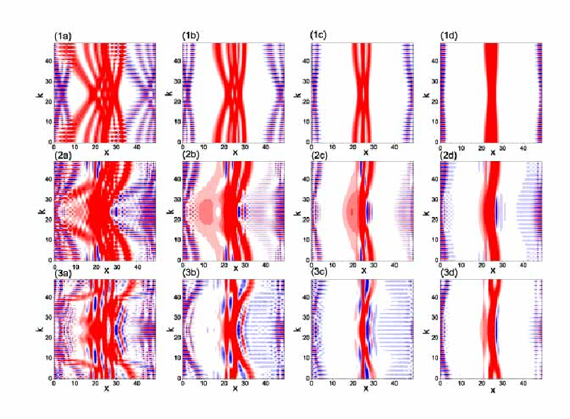
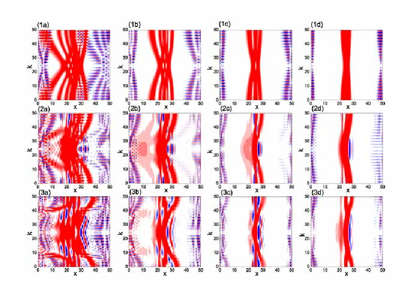
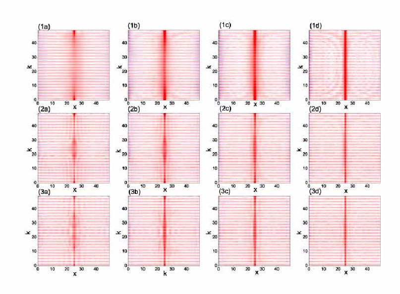
where is the disorder parameter. The exponential disorder in the above Equation has the advantage that the perturbed Hamilton possess a simple form in the Bloch representation, and analytical solutions may be possible using the perturbation theory. Here, we only give numerical results for the phase space structure for such disorder. Figs. 7 and 8 show the phase space structure on networks of size and for different values of and . The first column of the figures shows for on networks with , and (rows 1-3). For this weak disorder, the phase space patterns have a very strange structure and the patterns of the ordered networks are destroyed. Increasing the disorder parameter , the patterns change drastically. The phase space structure gets suppressed and a localized region forms at the initial node . In contrast to the patterns in Ref. [37], the Wigner function here has negative values on highly connected networks with large disorder (Compare the plots in the last column to plots in Ref. [37]). The patterns in phase space on odd-numbered networks (Fig. 8) have a similar structure as the even-numbered networks. However, differences are also visible and it seems that there are more stripes on even-numbered networks (Compare the corresponding plots in Fig. 7 and Fig. 8).
Compared to the patterns in Ref. [37], the phase space structure for networks with exponential disorder shows a strange patterns. Such difference is induced by the distinct type of disorder. The perturbed Hamiltonian in Ref. [37] has a Gauss form, such disorder leads to a symmetrical phase space pattern in the plane. Here, the exponential disorder has a heterogeneous strength, i.e., sites labeled as large numbers have large exponential disorder (See Eq. (17)), this heterogeneous disorder results in the complex pattern of the observed phase space. For larger disorder, the difference of phase space between networks with differen connectivity becomes invisible. We believe for sufficient strong disorder, the phase space displays a complete localization at the initial node.
III.2 topological disorder
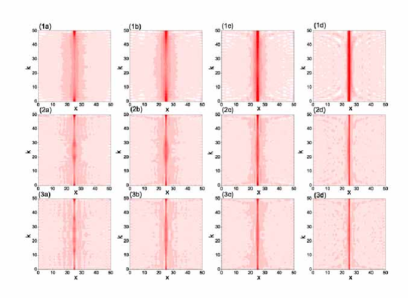
Since the topological structure of the WS model is not single, we average the time limiting Wigner function over distinct realizations. The ensemble average of the Wigner function provides us a holistic view on the phase space structure of disordered networks. Figs. 9 and 10 show the ensemble averaged phase space patterns on disorder networks of size and with different values of and . It is found that the stripes on regular networks are destroyed and localized regions form around the initial node (Compare Fig. 3 and Fig. 9). Increasing the rewiring probability (disorder parameter in the WS model), the patterns change profoundly. The phase space structure gathers together at the initial node for all on networks with large disorder. However, the stripes on ordered networks are still visible even for large disorder. When the disorder parameter is fixed, the effect of localization becomes weak on networks with more connectivity (Compare the plots in the same columns). For odd-numbered networks, the patterns of localized central regions are rather comparable to that on even-numbered networks. The other regions in the phase space are analogous to the patterns of the corresponding ordered networks, although the local patterns around the are changed.
Summing the averaged limiting Wigner function over gives the averaged transition probability . Fig. 11 shows this marginal distribution for even and odd with different connectivity and disorder strength. In the figure, we can see that there is a remarkable localization at the initial node when . As increases, the localizations become weak and nearly the same for and (Compare the corresponding dots and curves in row 2 and 3). Interestingly, we note that the marginal distributions on even and odd numbered networks are nearly the same and there is only one peak at . This feature differs from the case on ordered networks where there are two peaks ( and ) for even and only one peak () for odd . The two peak marginal distribution on regular even-numbered networks is a consequence of the symmetry of the network topology. When disorder was added, such topological symmetry is destroyed, resulting in the single-peaked marginal distributions on disordered networks.

IV Conclusions and Discussions
In conclusions, we have studied the quantum-mechanical phase space patterns on ordered and disordered networks. On ordered networks where each node connects to its nearest neighbors ( on either side), the phase space quasi-probability of Wigner function shows various patterns. In the long time limit, the phase space structure presents different kinds of stripes. Such striped patterns are related to the specific network size and connectivity parameter . Interestingly, if the network size is an even number, we find an asymmetric quasi-probability and transition probability between the node and its opposite node. This asymmetry depends on the network parameters and specific phase space positions. On disordered networks in which each edge is rewired with probability , the phase space displays regional localization on the initial node.
The asymmetry of the quasi-probability and transition probability is a novel phenomenon, which does not exist in the cycle graph with . However, we are unable to predict which particular parameters of and or which phase space positions () are related to such asymmetry. Is there relation between the phase space asymmetry and transition probability asymmetry? Such question is interesting and requires a further study. The phase space patterns on disordered networks suggest that there are localizations in phase space on small-world networks. Although both the static disorder and topological disorder lead to localizations at the initial node, localizations on small-world networks indicates that it is a generic property of disordered systems and has important consequences for quantum walk algorithms and quantum communication [38, 39].
Acknowledgements.
The authors would like to thank Zhu Kai for converting the mathematical package used in the calculations. This work is supported by the Cai Xu Foundation for Research and Creation (CFRC), National Natural Science Foundation of China under project 10575042 and MOE of China under contract number IRT0624 (CCNU).References
- [1] G. H. Weiss, Aspect and Applications of the Random Walk (North-Holland, Amsterdam, 1994).
- [2] J. Kempe, Contemp. Phys. 44, 307 (2002).
- [3] D. Supriyo, Quantum Transport: Atom to Transistor (Cambridge University Press, London, 2005).
- [4] A. Ambainis, Quantum search algorithms (New York, USA , 2004).
- [5] F. W. Strauch, Phys. Rev. A 74, 030301 (2006).
- [6] A. Ambainis, J. Kempe and A. Rivosh,Coins make quantum walks faster (Philadelphia, USA, 2005).
- [7] D. Solenov and L. Fedichkin, Phys. Rev. A 73, 012313 (2003)
- [8] T. Frankel, The geometry of physics: An introduction (Cambridge University Press, London, 2003).
- [9] W. K. Wootters, Ann. Phys. 176, 1 (1987)
- [10] O. Mülken and A. Blumen, Phys. Rev. A 73, 012105 (2006).
- [11] G. S. Agarwal and E. Wolf, Phys. Rev. D 2, 2161 (1970); ibid. 2, 2187 (1970); ibid. 2, 2206 (1970).
- [12] E. J. Heller, J. Chem. Phys. 65, 1289 (1976).
- [13] C. C. López and J.-P. Paz, Phys. Rev. A 68, 052305 (2003).
- [14] A. M. Smith and C. W. Gardiner, Phys. Rev. A 38, 4073 (1988).
- [15] P. Blanchard and J. Stubbe, Rev. Math. Phys. 8, 503 (1996).
- [16] M. V. Berry, Phil. Trans. R. Soc. London A 287, 237 (1977).
- [17] P. Carruthers and F. Zachariasen, Rev. Mod. Phys. 55, 245 (1983).
- [18] T. Miyazaki, M. Katori and N. Konno, Phys. Rev. A 76, 012332 (2007).
- [19] C. Mique, J.-P. Paz and M. Saraceno, Phys. Rev. A 65, 062309 (2002).
- [20] J. H. Hannay and M. V. Berry, Physica D 1, 267 (1980).
- [21] P. Bianucci, C. Miquel, J.-P. Paz and M. Saraceno, Phys. Lett. A 297, 253 (2002).
- [22] J.-P. Paz, Phys. Rev. A 65, 062311 (2002).
- [23] D. J. Watts and S. H. Strogatz, Nature 393, 267 (1998).
- [24] S. H. Strogatz, Nature 410, 268 (2001).
- [25] R. Albert and A.-L. Barabäsi, Rev. Mod. Phys. 74, 47 (2002).
- [26] S. N. DoroGovtsev and J. F. F. Mendes, Adv. Phys. 51, 1079 (2002).
- [27] S. Boccaletti, V. Latora, Y. Moreno, M. Chavez and D.-U. Hwang, Phys. Rep. 424, 175 (2006).
- [28] J. F. F. Mendes, S. N. DoroGovtsev and A. F. Ioffe, Evolution of Networks: From Biological Nets to the Internet and WWW (Oxford University Press, Oxford, 2003).
- [29] S. H. Strogatz, and I. Stewart, Sci. Am. 269, 102 (1993).
- [30] K. Wiesenfeld, Physica B 222, 315 (1996).
- [31] L. F. Abbott and C. V. Vreeswijk, Phys. Rev. E 48, 1483 (1993).
- [32] I.V. Belykh, V.N. Belykh and M. Hasler, Physica D 195, 159 (2004).
- [33] M. E. J. Newman and D. J. Watts, Phys. Rev. E 60, 7332 (1999).
- [34] C. Kittel, Introduction to solid state physics (Wiley, New York, 1986).
- [35] O. Mülken, A. Volta and A. Blumen, Phys. Rev. A 72, 042334 (2005)
- [36] A. Volta, O. Mülken and A. Blumen, J. Phys. A 39, 14997 (2006)
- [37] O. Mülken, A. Volta and A. Blumen, Phys. Rev. E 75, 031121 (2007)
- [38] J. P. Keating, N. Linden, J. C. F. Matthews and A. Winter, Phys. Rev. A 76, 012315 (2007).
- [39] P. W. Anderson, Phys. Rev. 109, 1492 (1958).