Structured environments in solid state systems: crossover from Gaussian to non-Gaussian behavior
Abstract
The variety of noise sources typical of the solid state represents the main limitation toward the realization of controllable and reliable quantum nanocircuits, as those allowing quantum computation. Such “structured environments” are characterized by a non-monotonous noise spectrum sometimes showing resonances at selected frequencies. Here we focus on a prototype structured environment model: a two-state impurity linearly coupled to a dissipative harmonic bath. We identify the time scale separating Gaussian and non-Gaussian dynamical regimes of the Spin-Boson impurity. By using a path-integral approach we show that a qubit interacting with such a structured bath may probe the variety of environmental dynamical regimes.
Keywords:
Decoherence, quantum statistical methods, quantum computationpacs
03.65.Yz, 03.67.Lx, 05.40.-aI Introduction
Controlled coherent dynamics of solid state devices has been demonstrated in recent years [1, 2]. Compared to other implementations, solid state qubits suffer from stronger broadband noise originating from sources with different character. The main limitation toward the realization of controllable and reliable quantum circuits allowing quantum computation is decoherence due to material (and device) dependent noise sources. The resulting noise spectrum is non-monotonous and sometimes characterized by resonances. Often these features may be attributed to interaction with a nonlinear and non-Markovian environment [3].
In superconducting nanocircuits a particularly detrimental role is played by fluctuating impurities located in the insulating material surrounding the qubit, which are responsible for charge noise and flux noise [4, 5]. Background charges are known to be responsible for low-frequency noise [6], moreover experiments with Josepshon devices suggested that spurious two-level systems may also affect high-frequency noise [7]. Connections between low and high-frequency noise features have been suggested in the recent experiment Ref. [8]. Different microscopic mechanisms [9] and effective models [10] have been recently proposed to explain the observed spectral features.
Predicting decoherence originating from such a structured environment often responsible for non-Gaussian noise is a non trivial task, which has attracted a lot of attention in the past years [3, 11, 12, 13, 14]. A well established scheme consists in studying the reduced dynamics of an extended system composed of the qubit and of the environmental degrees of freedom responsible for non-Gaussian behavior. This strategy, combined with an appropriate classification of the noise sources (i.e. adiabatic or quantum noise), each treated via appropriate approximate tools, provides a general scheme to deal with the variety of noise sources typical of the solid state [14, 15]. In this paper we focus on a prototype impurity model, a two-state impurity linearly coupled to a dissipative harmonic bath. Such Spin-Boson models have been thoroughly investigated with a variety of methods since the ’80s [16, 17]. Thus the impurity dynamics is well known in a wide region of parameters space. This allows the identification of the impurity characteristic time scales and, therefore, of the conditions where deviations from Gaussian and/or weak coupling regimes are expected. Having this information at our disposal we will apply standard techniques developed for quantum dissipative systems to find the qubit dynamics in the presence of this structured bath. The analysis will provide evidence for the appearance of non-Gaussian effects. In particular, their onset will be shown to be related to clearly identifiable effects in the qubit behavior.
In Section 2 we introduce the qubit-impurity model and identify the relevant impurity dynamical quantities. In Section 3 we review the equilibrium correlation function for a Spin-Boson impurity and identify its correlation time. In Section 4 we study the qubit dynamics in the presence of the Spin-Boson impurity within a path-integral approach and discuss the main features of the crossover from weak to strong coupling.
II Model and relevant dynamical quantities
To be specific we shall refer to superconducting qubits based on the Cooper-pair box [1, 18]. Under proper conditions the device behaves as a two-state system described in terms of Pauli matrices by ()
| (1) |
The charging energy gives the additional cost of adding an extra Cooper pair to the superconducting island and the possibility of coherent transfer of pairs through the junction is given by the Josephson term . The charge on the superconducting island may fluctuate because of interaction with uncontrolled impurities. Here we model a single impurity with a Spin-Boson model, the overall Hamiltonian being given by
| (2) | |||
| (3) |
The two-level-system impurity () is coupled to a harmonic bath, described by , via the collective coordinate . Its effect on the impurity depends only on the spectral density or equivalently on the power spectrum
| (4) | |||||
where denotes the thermal average with respect to , and . We consider the standard case when the coupling operator is a collective displacement with ohmic spectral density
| (5) |
where represents the high frequency cut-off of the harmonic modes.
A first step in understanding the effects of damping is to view the impurity and the ohmic bath as an environment for the qubit . This environment is in general non-Gaussian and non-Markovian. A Gaussian approximation of this structured bath amounts to replace it with an effective harmonic model directly coupled to and with power spectrum
| (6) |
the Fourier transform of equilibrium symmetrized auto-correlation function of the impurity observable which directly couples to the qubit. Here the thermal average is performed with respect to and is the thermal equilibrium value for . Under this approximation and using a master equation approach, the relaxation and dephasing rates for the qubit in lowest order in the coupling read [17, 20],
| (7) | |||||
| (8) | |||||

where is the qubit splitting. The validity of this standard approach is limited to couplings [20], where is the range of the correlation function in Eq.(6) (to be defined in the next Section). Clearly if the impurity has a slow dynamics , this picture does not apply and we have to resort to other methods. However previous studies on a similar model have shown that the Gaussian approximation may give good results even for but for shorter and shorter times, as long as increases [3].
¿From a different perspective the failure of the Gaussian approximation can be understood by viewing the qubit as a measuring device [21] for the mesoscopic system described by the Spin-Boson model involving . A rather rough measurement protocol (short times, averaging of results) makes the dynamics of essentially sensitive only to , whereas if the Spin-Boson has a slow dynamics the spin is able to detect also details of the dynamics of which go beyond , and have to be described with more careful methods.
In the following we will treat the impurity on the same footing as the qubit , we will apply standard methods to trace out the bosonic degrees of freedom without any approximation on the qubit-impurity coupling.
III Impurity dynamics and correlation time
In this Section we will identify the characteristic time scale of the dynamics of the equilibrium fluctuations of the Spin-Boson impurity described by Eq.(6). The uncoupled (i.e. for ) impurity dynamics strictly depends on the damping strenght and on the temperature [17]. We consider the small damping regime where series of crossovers from under-damped to over-damped oscillations and to relaxation dynamics with increasing temperature are observed. This analysis is also relevant to understand the effect of ensemble of impurities when a wide distribution of parameters has to be taken into account as in Ref. [10]. In fact at any fixed temperature each impurity may display a specific dynamical behavior. As a consequence, various sets of impurities may effect the qubit dynamics in qualitatively different ways.
Our goal is to establish to which extent the qubit may probe the variety of regimes of its environment dynamics. The important scale allowing the identification of Gaussian/non-Gaussian dynamical regimes is extracted from the equilibrium auto-correlation function of the observable which directly couples to the qubit. We remark that the thermal initial state of the Spin-Boson system, which is implied by the equilibrium correlation function, may originate peculiar time-dependencies. Qualitatively different behaviors may in fact be displayed by the non-equilibrium correlation function, which is evaluated for a factorized initial state of the Spin-Boson system [17, 19]. Evaluation of equilibrium correlation functions for the Spin-Boson model is a non trivial task. However it has been shown [17] that in the unbiased case , and for small damping , the auto-correlation function does not depend on the initial correlated or factorized state. Here we focus on this case and recall the characteristics of more relevant for our analysis, the interested reader may find details of the derivation in Refs. [17, 19].

The crossover from under-damped to over-damped behavior with increasing temperature takes place at
| (9) |
where is the renormalized tunneling amplitude in the Spin-Boson model.
The explicit form for depends on temperature[22]
For it reads
| (10) |
where . The effective frequency and the relaxation rate are
| (12) |
for temperatures and
| (13) | |||||
| (14) |
for larger temperatures .
Here is the white noise level for frequencies in (4). Oscillators with frequencies renormalize the tunneling amplitude to
| (15) |
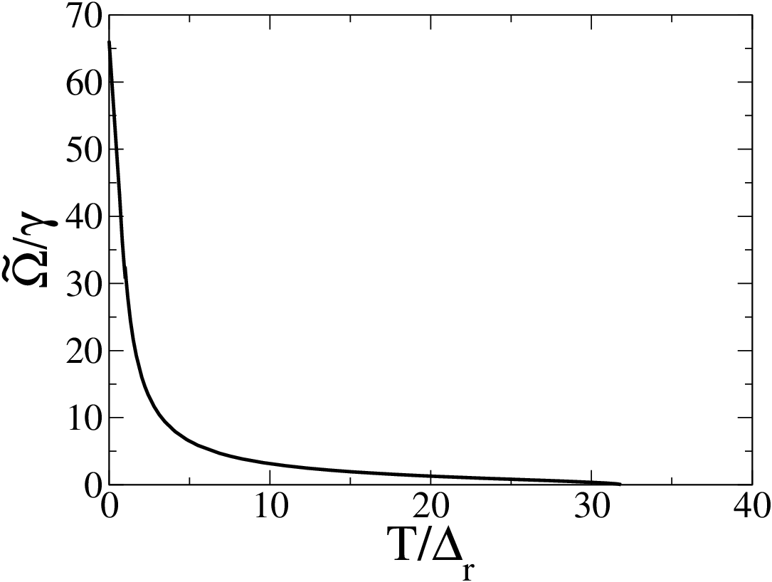
In Fig.1 we show the overall behavior of . At very small temperatures (see inset in Fig.1) increases . The two forms () and (13) smoothly match on each other at . A maximum is reached at , above this temperature decreases monotonously and approaches zero at . Coherent oscillations are dephased on a scale which decreases monotonously starting from . The resulting quality factor of the damped oscillations is shown in Fig.2.
For temperatures higher than the dynamics is incoherent and has a different form
| (16) | |||||
| (17) |
Note that for one of the two rates increases with temperature, , whereas the other shows the characteristic Kondo behavior, decreasing with temperature
| (18) |
These features are illustrated in Fig.3.
The typical scale of the equilibrium fluctuactions of the Spin-Boson environment described by defines the correlation time . Usually in the literature one is faced with environment models characterized by dynamic fluctuations which tend rapidly to zero with time. In these cases represents the order of magnitude of the width of the environment fluctuactions [20]. In the present case however looking at the Spin-Boson impurity as an environment characterized by the identification of is not immediate due to the different forms of the equilibrium fluctuations given by Eqs.(10) and (16). For high temperatures is approximately a single Lorentzian centered at and width , leading to the identification , see Fig.4.


In the opposite limit of very low temperatures has a double peak structure representing a bath responsible for oscillating fluctuations very weakly damped. In this unusual environment regime, the typical scale of the impurity fluctuations is represented by which plays the role of . For intermediate temperatures in general two almost superimposed Lorentzians contribute to and may be approximately identified from the condition . The resulting , illustrated in Fig.5, interpolates between the asymptotic behaviors at low and high temperatures. The slight reduction of at intermediate temperatures is a consequence of the crossover from under-damped to incoherent dynamics, as shown in Fig.4.
Once the impurity correlation time is identified, the condition separates the weak-coupling regime of the qubit dynamics, from the strong coupling regime where non-Gaussian behavior shows up. In the first case, when , the standard master equation predicts exponential decay with the Golden Rule rate given in Eq.(8). ¿From the above analysis we expect the master equation result to be valid in the following regimes: For temperatures if , for larger temperatures if , this condition can be cast in the following form
| (19) |
Therefore, for small values of a crossover from weak to strong coupling is expected with increasing temperature. For the ensuing discussion here we report the expected value of the pure dephasing rate with Eqs.(10) and (16)
| (20) | |||||
| (21) |
The two forms match on each other at , and it is easy to show that Eq.(21) approximates also for .

IV Qubit dynamics: path-integral approach
The discussion of the previous Section has evidenced the existence of a large parameter regime where the Gaussian approximation of the Ohmic Spin-Boson model does not apply. In this Section we study the qubit dynamics via a path-integral approach which includes as a special case the regime of Gaussian behavior of the impurity dynamics. We find exact expressions which we discuss for finite temperatures, specifically for .
We focus on the so called pure-dephasing regime, , which represents the point of maximum noise sensitivity of the qubit. Thus the more interesting in the perspective of using the qubit as a “noise” analyzer. In the pure dephasing regime the charge on the qubit island is a constant of motion since , dephasing being described by the decay of or equivalently of the coherences . A simple analysis shows that the coherences are related to correlation functions involving the Spin-Boson variables, specifically we found [3, 23]


| (22) | |||||
where we have chosen a factorized initial density matrix for the qubit-impurity, , with the impurity initialized in the mixed state and the bosonic bath in its thermal equilibrium state . The two conditional impurity Hamiltonians depend on the qubit state and read .
In Ref. [23] it has been shown that the Laplace transform of the correlator reads
| (23) | |||||
| (24) |


An exact formal series expression in for the kernels , has been derived in Ref.[23]. In the Markovian regime for the harmonic bath, i.e. for and temperatures , all contributions to and of order higher than cancel out exactly. The lowest order contributions [25] do not depend on the coupling and coincide with the kernels entering the dynamics of in the uncoupled case () [17] which read
| (25) | |||||
| (26) |
Inserting Eqs.(25) - (26) in (23) and (24) is readily found as
The scales entering the time evolution of are found from the solution of the pole equation , which have been reported in Ref.[15]. Here we specify to the unbiased case , the goal being to elucidate the correspondence with the expected Gaussian/non-Gaussian dynamical regimes as deduced from the equilibrium correlation function discussed in Section III.


IV.1 Pure dephasing due to a unbiased impurity
When the pole condition with Eq.(IV) reduces to a cubic equation which has either one real and two complex conjugate solutions, or three real solutions. We denote the three roots as and , where is either real or purely imaginary. The expression of in terms of the is obtained by inverting the Laplace transform (IV) and reads
| (34) | |||
| (35) |
It is possible to show that the character of the roots depends on and on the temperature. In particular for we can identify two temperatures
| (36) | |||||
such that for and one solution is real and two are complex conjugate, whereas for intermediate temperatures the three solutions are real. For there is always one real and two complex conjugate solutions. Analytic expressions for the roots are quite cumbersome, approximate forms have been reported in [23]. Here we discuss the physically relevant regimes where crossover are expected in the behavior of . To this end we focus on the dominant , i.e. the smallest in absolute value. The analysis is conveniently performed distinguishing regimes where or


Case In this regime the characteristics of the dominant pole change qualitatively with increasing temperatures (with lower bound ). For temperatures low enough to fulfill the condition
| (37) |
the dominant scale is real and reads . In (35) and therefore
| (38) |
With increasing temperature, above the dominant scales are complex conjugate, . Figure 6 illustrates the crossover between the two regimes for . Since and , we get
| (39) |
As expected, for small enough temperature the Gaussian approximation for the structured bath applies
and a single scale dominates the qubit dynamics.
It is easily seen that the condition (37)
corresponds to (19) which was derived from the weak coupling
criterion . Moreover as given in
Eq.(21).
For higher temperature non Gaussian effects show up. The qualitative change is characterized by
damped oscillations at frequency in as shown in Fig.7, and
beatings at frequencies in the coherences Eq.(22).
Note that the coupling strength only enters the induced frequency shift, whereas the decay
rate shows the Kondo behavior , cfr Eq.(18).
Case For larger values of the system stays in the regime where the dominant scales are complex conjugate and show a nontrivial temperature dependence. At temperatures , the two poles read , with increasing instead . The qubit dynamics follows Eq.(39). The dominant rate is non-monotonous first increasing with temperature and than decreases . For large enough temperatures the decay of the coherences does not depend on , as expected.
This qualitative behavior is already present for intermediate values of , as shown in Fig.8. The poles never cross, therefore there is no change in the character of the qubit dynamics. In the specific case considered at small/intermediate temperatures the real parts of the three poles are of the same order. This is reflected in the Fourier transform of where three Lorentzians can be identified, one centered at , the others at , see Fig.9.
V Discussion
The presented analysis has shown that a damped impurity may behave as an effective short-time correlated or as a non-Gaussian environment depending both on its coupling with the qubit and on temperature. The relevant scale separating the two regimes is given by . In Section III the correlation time of the unbiased Spin-Boson model has been found for small damping at any temperature. We have shown that the qubit may act as a detector of non-Gaussian dynamical behavior, the most evident effect being the occurrence of beatings which are expected with increasing temperature. We remark that the results we have illustrated have been derived within the NIBA which limits temperatures to values larger than . A interesting issue is to analyse the small temperature regime where we expect that crossover effects may take place also for large values of . A detailed analysis of the low temperature regime can be performed within the systematic weak damping approximation [17] and will be reported elsewhere [24].
References
- [1] Y. Nakamura, Yu.A. Pashkin, J.S. Tsai, Nature 398, 786 (1999).
- [2] Y. Nakamura et al., Phys. Rev. Lett. 88, 047901 (2002); D. Vion et al., Science 296, 886 (2002); Y. Yu et al., Science 296, 889 (2002); J. Martinis et al., Phys. Rev. Lett. 89, 117901 (2002); J. Friedman et al., Nature 406, 43 (2000); I. Chiorescu et al., Science, 299, 1869 (2003); Yu. A. Pashkin et al., Nature 421, 823 (2003).
- [3] E. Paladino et al., Phys. Rev. Lett. 88, 228304 (2002); G. Falci et al., Proceedings of the International School Enrico Fermi on ”Quantum Phenomena of Mesoscopic Systems”, B. Altshuler and V. Tognetti Eds., IOS Bologna (2003). E. Paladino, L. Faoro, G. Falci, Adv. Solid State Phys. 43, 747 (2003).
- [4] Y. Nakamura, Yu.A. Pashkin,T. Yamamoto J.S. Tsai, Phys. Rev. Lett., 88, 047901 (2002).
- [5] G. Ithier, et al., Phys. Rev. B, 72, 134519 (2005)
- [6] G. Zimmerli, T. M. Eiles, R.L. Kautz, J.M. Martinis, Appl. Phys. Lett., 61, 237 (1992); S. M. Verbrugh et al., 78, 2830 (1995); A.B. Zorin et al., Phys. Rev. B 53, 13682 (1996); V. A. Krupenin et al., J. Appl. Phys. 84, 3212 (1998).
- [7] R. W. Simmonds et al., Phys. Rev. Lett. 93, 077003 (2004).
- [8] O. Astafiev et al., Phys. Rev. Lett. 93, 267007 (2004).
- [9] L. Faoro, J. Bergli, B. L. Altshuler, and Y. M. Galperin, Phys. Rev. Lett. 95, 046805 (2005); L. Faoro, L. Ioffe, Phys. Rev. Lett. 96, 047001 (2006); I. Martin and Y.M. Galperin, Phys. Rev. B, 73, 18021R (2006)
- [10] A. Shnirman et al., Phys. Rev. Lett. 94, 127002 (2005).
- [11] H. Gassmann, F. Marquardt, C. Bruder, Phys. Rev. E, 66, 041111 (2002).
- [12] Y. Makhlin and A. Shnirman, Phys. Rev. Lett. 92, 178301 (2004).
- [13] Y. M. Galperin, B. L. Altshuler, J. Bergli, and D. V. Shantsev Phys. Rev. Lett. 96, 097009 (2006)
- [14] G. Falci et al., Phys. Rev. Lett. 94, 167002 (2005)
- [15] E. Paladino, M. Sassetti, G. Falci, U. Weiss, Chem. Phys.322, 98 (2006).
- [16] A. Leggett et al., Rev. Mod. Phys. 59, 1 (1987).
- [17] U. Weiss Quantum Dissipative Systems 2nd Ed (World Scientific, Singapore 1999).
- [18] Y. Makhlin, G. Schön, and A. Shnirman Rev. Mod. Phys. 73, 357 (2001) and references therein.
- [19] M. Sassetti and U. Weiss, Phys. Rev. Lett. 65, 2262 (1990); M. Sassetti and U. Weiss, Phys. Rev. A 41, 5383 (1990).
- [20] C. Cohen-Tannoudji, J. Dupont-Roc and G. Grynberg Atom-Photon Interactions, Wiley-Interscience (1993).
- [21] R. Aguado and L.P Kouwenhoven, Phys. Rev. Lett. 84, 1986 (2000); M. H. Devoret and R. J. Schoelkopf, Nature 406, 1039 (2000).
- [22] The above analytic forms have been derived in Ref. [17] within the so called Non-Interacting-Blip-Approximation (NIBA) which is exact in the considered regime ( and ).
- [23] E. Paladino, M. Sassetti, G. Falci, Chem. Phys., 296, 325 (2004).
- [24] E. Paladino et al., in preparation 2007.
- [25] In the Spin-Boson literature the approximation of the kernels to order is referred to as Noninteracting-Blip-Approximation (NIBA). It’s validity regimes include the considered Markovian case and [17].