Reconstruction of Longitudinal Profiles of Ultra-High Energy Cosmic Ray Showers from Fluorescence and Cherenkov Light Measurements
Abstract
We present a new method for the reconstruction of the longitudinal profile of extensive air showers induced by ultra-high energy cosmic rays. In contrast to the typically considered shower size profile, this method employs directly the ionization energy deposit of the shower particles in the atmosphere. Due to universality of the energy spectra of electrons and positrons, both fluorescence and Cherenkov light can be used simultaneously as signal to infer the shower profile from the detected light. The method is based on an analytic least-square solution for the estimation of the shower profile from the observed light signal. Furthermore, the extrapolation of the observed part of the profile with a Gaisser-Hillas function is discussed and the total statistical uncertainty of shower parameters like total energy and shower maximum is calculated.
Keywords:
Cosmic rays , extensive air showers , air shower reconstruction , air fluorescence , Cherenkov lightPACS
96.50.sd, , , and
1 Introduction
The particles of an extensive air shower excite nitrogen molecules in the atmosphere, which subsequently radiate ultraviolet fluorescence light isotropically. This fluorescence light signal can be measured with appropriate optical detectors such as the fluorescence telescopes of HiRes [1], the Pierre Auger Observatory [2] or the Telescope Array [3].
The number of emitted fluorescence photons is expected to be proportional to the energy deposited by the shower particles. Recent measurements of the fluorescence yield in the laboratory confirm this expectation within the experimental uncertainties [4, 5, 6]. Non-radiative processes of nitrogen molecule de-excitation lead to a temperature, pressure and humidity dependence of the fluorescence yield (see e.g. [7]). For atmospheric parameters of relevance to the reconstruction of air showers of ultra-high energy cosmic rays, the pressure dependence of the ionization energy deposit per meter track length of a charged particle is almost perfectly canceled by the pressure dependence of the fluorescence yield (see, for example, [8]). Therefore only a weak pressure and temperature dependence has to be taken into account if the number of emitted photons is converted to a number of charged particle times track length, as has been done in the pioneering Fly’s Eye experiment [9]. The reconstructed longitudinal shower profile is then given by the number of charged particles as function of atmospheric depth.
The approximation of assuming a certain number of fluorescence photons per meter of charged particle track and the corresponding expression of the longitudinal shower development in terms of shower size are characterized by a number of conceptual shortcomings. Firstly the energy spectrum of particles in an air shower changes in the course of its development. A different rate of fluorescence photons per charged particle has to be assumed for early and late stages of shower development as the ionization energy deposit depends on the particle energy [10]. Secondly the tracks of low-energy particles are not parallel to the shower axis leading to another correction that has to be applied [11]. Thirdly the quantity “shower size” is not suited to a precise comparison of measurements with theoretical predictions. In air shower simulations, shower size is defined as the number of charged particles above a given energy threshold that cross a plane perpendicular to the shower axis. Setting this threshold very low to calculate the shower size with an accuracy of % leads to very large simulation times as the number of photons diverges for . Moreover, the shower size reconstructed from data depends on simulations itself since the shower size is not directly related to the fluorescence light signal.
These conceptual problems can be avoided by directly using energy deposit as the primary quantity for shower profile reconstruction as well as comparing experimental data with theoretical predictions. Due to the proportionality of the number of fluorescence photons to the energy deposit, shower simulations are not needed to reconstruct the total energy deposit at a given depth in the atmosphere. Another advantage is that the calorimetric energy of the shower is directly given by the integral of the energy deposit profile [12]. Furthermore the energy deposit profile is a well-defined quantity that can be calculated straight-forwardly in Monte Carlo simulations and does not depend on the simulation threshold [13].
Most of the charged shower particles travel faster than the speed of light in air, leading to the emission of Cherenkov light. Thus, in general, the optical signal of an air shower consists of both fluorescence and Cherenkov light contributions. In the traditional method [9] for the reconstruction of the longitudinal shower development, the Cherenkov light is iteratively subtracted from the measured total light. The drawbacks of this method are the lack of convergence for events with a large amount of Cherenkov light and the difficulty of propagating the uncertainty of the subtracted signal to the reconstructed shower profile.
An alternative procedure, used in [14], is to assume a functional form for the longitudinal development of the shower, calculate the corresponding light emission and vary the parameters of the shower curve until a satisfactory agreement with the observed light at the detector is obtained. Whereas in this scheme the convergence problems of the aforementioned method are avoided, its major disadvantage is that it can only be used if the showers indeed follow the functional form assumed in the minimization.
It has been noted in [15] that, due to the universality of the energy spectra of the secondary electrons and positrons within an air shower, there exists a non-iterative solution for the reconstruction of a longitudinal shower profile from light detected by fluorescence telescopes.
Here we will present an analytic least-square solution for the estimation of the longitudinal energy deposit profile of air showers from the observed light signal, in which both fluorescence and Cherenkov light contributions are treated as signal. We will also discuss the calculation of the statistical uncertainty of the shower profile, including bin-to-bin correlations. Finally we will introduce a constrained fit to the detected shower profile for extrapolating it to the regions outside the field of view of the fluorescence telescope. This constrained fit allows us to always use the full set of profile function parameters independent of the quality of the detected shower profile.

2 Fluorescence and Cherenkov Light Signals
The non-scattered, i.e. directly observed fluorescence light emitted at a certain slant depth is measured at the detector at a time . Given the fluorescence yield [4, 16, 17, 5] at this point of the atmosphere, the number of photons produced at the shower in a slant depth interval is
| (1) |
Here, denotes the energy deposited per unit depth at slant depth (cf. Fig. 1) and is defined as
| (2) |
where is the energy deposit per unit volume and () are cylinder coordinates with the shower axis at . The distance interval along the shower axis is given by the slant depth interval . The fluorescence yield is the number of photons expected per unit deposited energy for the atmospheric pressure and temperature at slant depth . The photons from Eq. (1) are distributed over a sphere with surface , where denotes the distance of the detector. Due to atmospheric attenuation only a fraction of them reach the detector aperture with area . Given a light detection efficiency of , the measured fluorescence light flux can be written as
| (3) |
where the abbreviation
is used. For the sake of clarity
the wavelength dependence of , and
will be disregarded in the following, but discussed later.
The number of Cherenkov photons emitted at the shower is proportional to the
number of charged particles above the Cherenkov threshold energy. Since the
electromagnetic component dominates the shower development, the emitted Cherenkov light,
, can be calculated from
| (4) |
where denotes the number of electrons and positrons above a certain energy cutoff, which is constant over the full shower track and not to be confused with the Cherenkov emission energy threshold. Details of the Cherenkov light production like these thresholds are included in the Cherenkov yield factor [15, 18, 19, 20].
Although Cherenkov photons are emitted in a narrow cone along the particle direction, they cover a considerable angular range with respect to the shower axis, because the charged particles are deflected from the primary particle direction due to multiple scattering. Given the fraction of Cherenkov photons per solid angle emitted at an angle with respect to the shower axis [18, 20], the light flux at the detector aperture originating from direct Cherenkov light is
| (5) |
Due to the forward peaked nature of Cherenkov light production, an intense Cherenkov light beam builds up along the shower as it traverses the atmosphere (cf. Fig. 1). If a fraction of the beam is scattered towards the observer it can contribute significantly to the total light received at the detector. In a simple one-dimensional model the number of photons in the beam at depth is just the sum of Cherenkov light produced at all previous depths attenuated on the way from to by :
| (6) |
Similar to the direct contributions, the scattered Cherenkov light received at the detector is then
| (7) |
Finally, the total light received at the detector at the time is obtained by adding the scattered and direct light contributions:
| (8) |
3 Analytic Shower Profile Reconstruction
The aim of the profile reconstruction is to estimate the energy deposit and/or electron profile from the light flux observed at the detector. At first glance this seems to be hopeless, since at each depth there are the two unknown variables and , and only one measured quantity, namely . Since the total energy deposit is just the sum of the energy loss of electrons, and are related via
| (9) |
where denotes the normalized electron energy distribution and is the energy loss per unit depth of a single electron with energy . As is shown in [15, 19, 20], the electron energy spectrum is universal in shower age , i.e. it does not depend on the primary mass or energy, but only on the relative distance to the shower maximum, . Eq. (9) can thus be simplified to
| (10) |
where is the average energy deposit per unit depth per electron at shower age . Parameterizations of can be found in [10, 20]. With this one-to-one relation (Eq. 10) between the energy deposit and the number of electrons, the shower profile is readily calculable from the equations given in the last section. For the solution of the problem, it is convenient to rewrite the relation between energy deposit and light at the detector in matrix notation: Let be the -component vector (histogram) of the measured photon flux at the aperture and the energy deposit vector at the shower track. Using the expression
| (11) |
the elements of the Cherenkov-fluorescence matrix can be found by a comparison with the coefficients in equations (3), (5) and (7):
| (12) |
where
| (13) |
and
| (14) |
The solution of Eq. (11) can be obtained by inversion, leading to the energy deposit estimator :
| (15) |
Due to the triangular structure of the Cherenkov-fluorescence matrix the inverse can
be calculated quickly even for matrices with large dimension. As the matrix elements in Eq. (12)
are always , is never singular.
The statistical uncertainties of are obtained by error propagation:
| (16) |
It is interesting to note that even if the measurements are uncorrelated, i.e. their
covariance matrix is diagonal, the calculated energy loss values
are not. This is
because the light observed during time interval
does not solely originate from , but also receives
a contribution from earlier shower parts , ,
via the ’Cherenkov light beam’.
4 Wavelength Dependence
Until now it has been assumed that the shower induces light emission at a single wavelength . In reality, the fluorescence yield shows distinct emission peaks and the number of Cherenkov photons produced is proportional to . In addition the wavelength dependence of the detector efficiency and the light transmission need to be taken into account. Assuming that a binned wavelength distribution of the yields is available (), the above considerations still hold when replacing and in Eq. (12) by
| (17) |
and
| (18) |
where
| (19) |
The detector efficiency and transmission coefficients and are evaluated at the wavelength .
5 Validation with Air Shower Simulations
In order to test the performance of the reconstruction algorithm we will use in the following
simulated fluorescence detector data.
For this purpose we generated proton air showers with an energy of 1019 eV
with the CONEX [21] event generator. The resulting
longitudinal charged particle and energy deposit profiles were
subsequently fed into the atmosphere and detector simulation package [22] of
the Pierre Auger Observatory.
The geometry and profile of the events in this simulated data sample was then reconstructed
within the Auger offline software framework [23].
Only events satisfying basic quality selection criteria have been used in the analysis.
In order to assure a good reconstruction of the shower geometry, the angular length
of the shower image on the camera was required to be larger than nine degrees. Moreover,
we only selected events with at least one coincident surface detector tank (so-called hybrid
geometry reconstruction [24]).
Furthermore we rejected under-determined measured longitudinal profiles by demanding
an observed slant depth length of 300 g cm-2 and a reconstructed
shower maximum within the field of view of the detector.
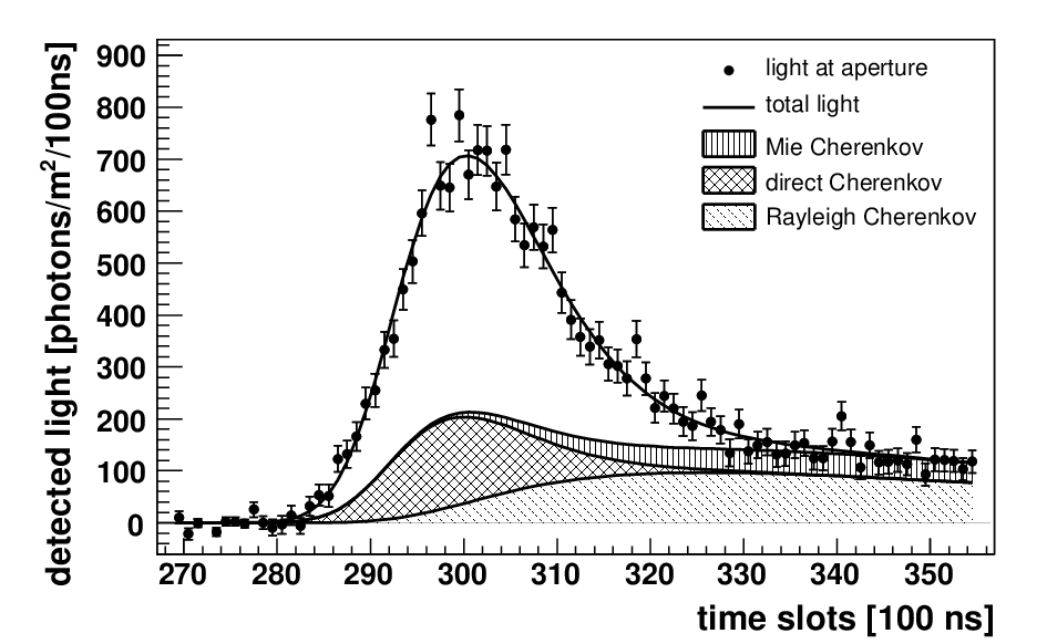
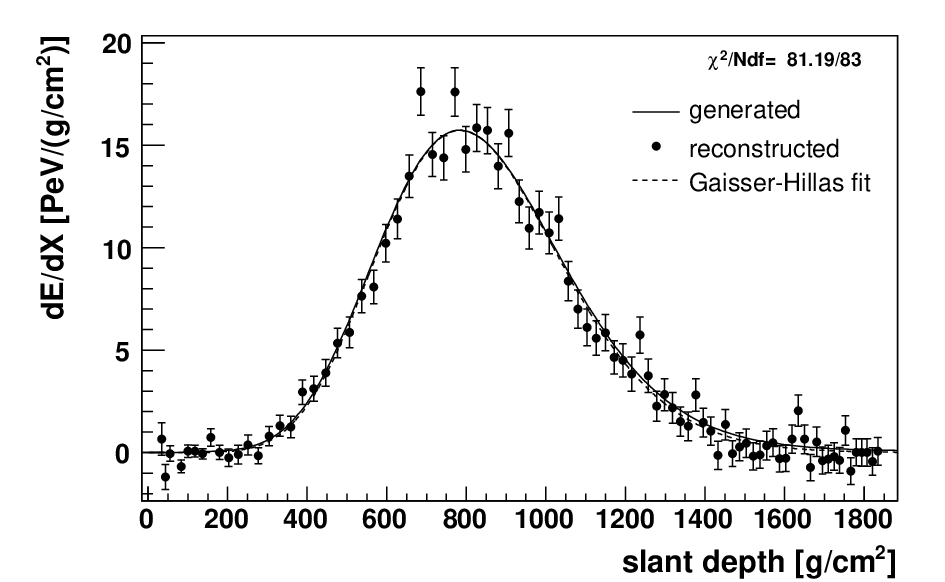
An example of a simulated event is shown in Fig. 2, illustrating
that the shape of the light curve at the detector can differ considerably from the
one of the energy deposit profile due to the scattered Cherenkov light
detected at late stages of the shower development. The reconstructed energy deposit curve,
however, shows on average a good agreement with the generated profile.
Since longitudinal air shower profiles exhibit similar shapes when transformed from slant depth
to shower age (see for instance [25]),
a good test of the profile reconstruction performance is to compare
the average generated and reconstructed energy deposit profiles as a function of
normalized to the energy deposit at shower maximum.
As can be seen in Fig. (3), the difference between these averages
is 1.5% and it can be concluded that the matrix method introduced here
performs well in reconstructing air shower profiles without a prior assumption
about their functional shape.

6 Shower Age Dependence
Due to the age dependence of the electron spectra , the Cherenkov yield factors and the average electron energy deposits depend on the depth of shower maximum, which is not known before the profile has been reconstructed. Fortunately, these dependencies are small: In the age range of importance for the shower profile reconstruction () varies by only a few percent [20] and by less than 15% [15]. Therefore, a good estimate of and can be obtained by setting over the full profile or by estimating from the position maximum of the detected light profile. After the shower profile has been calculated with these estimates, can be determined from the energy deposit profile and the profile can be re-calculated with an updated Cherenkov-fluorescence matrix. The convergence of this procedure is shown in Fig. 5. After only one iteration the (energy) differs by less than 0.1 g cm-2 (0.1%) from its asymptotic value. Note that age dependent effects of the lateral spread of the shower on the image seen at the detector [26, 27], though not discussed in detail here, have also been included in the simulation and reconstruction.
7 Gaisser-Hillas Fit


A knowledge of the complete profile is required for the calculation of the Cherenkov beam and the shower energy. If due to the limited field of view of the detector only a part of the profile is observed, an appropriate function for the extrapolation to unobserved depths is needed. A possible choice is the Gaisser-Hillas function [28]
| (20) |

which was found to give a good description of measured longitudinal profiles [29].
It has four free parameters:
, the depth where the shower reaches its maximum energy deposit
and two shape parameters and .
The best
set of Gaisser-Hillas parameters can be obtained by minimizing
the error weighted squared difference between the vector of function
values and , which is
| (21) |
This minimization works well if a large fraction of the shower has been observed below and above the shower maximum. If this is not the case, or even worse, if the shower maximum is outside the field of view, the problem is under-determined, i.e. the experimental information is not sufficient to reconstruct all four Gaisser-Hillas parameters. This complication can be overcome by constraining and to their average values and . The new minimization function is then the modified
| (22) |
where the variances of and around their mean values are in the denominators.
In this way, even if is not sensitive to and , the minimization
will still converge. On the other hand, if the measurements have small statistical uncertainties and/or
cover a wide range in depth, the minimization function is flexible enough to allow for
shape parameters differing from their mean values. These mean values can be determined
from air shower simulations or, preferably, from high quality data profiles which can be
reconstructed without constraints.
Eq. (22) can be
easily extended to incorporate correlations between and and
the energy dependence of their mean values.
Air shower simulations indicate a small logarithmic energy dependence of the
latter ( 25% and 5% per decade for and respectively [30]).
In practice it is sufficient to use energy independent values determined at low energies,
because at high energies the number of measured points is large and thus the constraints
do not contribute significantly to the overall .
The accuracy of the reconstructed energy, obtained by integrating over the
Gaisser-Hillas function (see below), and that of the depth of shower maximum, are displayed in Fig. 4 as a function
of the relative amount of Cherenkov light.
Note that the good resolutions of 7% and 20 g cm-2 are of course not
a feature of the reconstruction method alone, but depend strongly on the
detector performance and quality selection. The mean values of difference
to the true shower parameters, however, which are
close to zero for both fluorescence and Cherenkov light dominated events, indicate
that both light sources are equally suited to reconstruct the longitudinal development
of air showers.
A slight deterioration of the resolutions can be seen for events with a very small
Cherenkov contribution of 10%.
Such showers are either inclined events which developed high in the atmosphere where
the light scattering probabilities are low or deep vertical showers, for which most
of the late part of the shower is below ground level. Both topologies result in
a somewhat worse resolution: The former correspond to larger than average distances to the detector
and the latter to shorter observed profiles.
8 Error Propagation
A realistic estimate of the statistical uncertainties of important shower parameters is desired for many purposes, like data quality selection cuts, or the comparison between independent measurements like the surface and fluorescence detector measurements of the Pierre Auger Observatory or the Telescope Array. The uncertainties of , , and obtained after the minimization of Eq. (22), reflect only the statistical uncertainty of the light flux, which is why these errors will be referred to as ’flux uncertainties’ () in the following. Additional uncertainties arise from the uncertainties on the shower geometry (), atmosphere () and the correction for invisible energy ().
8.1 Flux uncertainty of the calorimetric energy
Even with the flux uncertainties of the Gaisser-Hillas parameters it is not straightforward to calculate the flux uncertainty of the calorimetric energy, which is given by the integral over the energy deposit profile:
| (23) |
To solve this integral one can substitute
| (24) |
in the Gaisser-Hillas function Eq. (20) to get
| (25) |
which can be identified with a Gamma distribution. Therefore, the above integral is given by
| (26) |
where denotes the Gamma-function. Thus, instead of doing a tedious error propagation to determine the statistical uncertainty of one can simply use it directly as a free parameter in the fit instead of the conventional factor :
| (27) |
In this way, is obtained directly from the contour of Eq. (22).
8.2 Geometric uncertainties
Due to the uncertainties on the shower geometry, the distances to
each shower point are only known within a limited precision and correspondingly the energy deposit
profile points are uncertain due to the transmission factors
and geometry factors . Furthermore, the uncertainty of the
shower direction, especially the zenith angle , affects
the slant depth calculation via and thus .
Finally, the amount of direct and scattered Cherenkov light depends on the shower geometry, too,
via the angles .
The algorithms used to reconstruct the shower geometry from fluorescence detector data usually determine the following five parameters [9], irrespective of whether the detectors operate in monocular, stereo or hybrid mode:
| (28) |
and are the angles of the normal vector of a plane spanned by the
shower axis and the detector (the so called shower-detector-plane), denotes the angle
of the shower within this plane and and are the time and distance of the shower
at its point of closest approach to the detector.
For any function standard error propagation yields the geometric uncertainty
| (29) |
where denotes the covariance matrix of the axis parameters. As the calorimetric energy and depend non-trivially on the shower geometry, the above derivatives need to be calculated numerically, i.e. by repeating the profile reconstruction and Gaisser-Hillas fitting for the ten new geometries given by to obtain
| (30) | |||||
with which Eq. (29) reads as
| (31) |
where
| (32) |
denote the correlation coefficients of the geometry parameters and .


8.3 Atmospheric uncertainties
Whereas the Rayleigh attenuation is a theoretically well understood process, the molecular density profiles and aerosol content of the atmosphere vary due to environmental influences and need to be well monitored in order to determine the slant depth and transmission coefficients needed for the profile reconstruction. Uncertainties in these measured atmospheric properties (see for instance [31, 32]) can be propagated in the same way as the geometric uncertainties by determining the one sigma shower parameter deviations via Eq. (30).
8.4 Invisible energy
Not all of the energy of a primary cosmic ray particle ends up in the electromagnetic part of an air shower. Neutrinos escape undetected and muons need long path lengths to fully release their energy. This is usually accounted for by multiplying the calorimetric energy, Eq. (23), with a correction factor determined from shower simulations to obtain the total primary energy
| (33) |
The meson decay probabilities, and thus the amount of neutrino and muon production, decrease with energy, therefore depends on the primary energy. For instance, in [33] it is parameterized as
| (34) |
where , and denote constants depending on the primary composition and interaction model assumed11 1 Note that here only the statistical uncertainties of the invisible energy correction are discussed. For an estimate on the related systematic uncertainties see [34]. This energy dependence needs to be taken into account when propagating the calorimetric energy uncertainty to the total energy uncertainty.
Due to the stochastic nature of air showers, the correction factor is subject to shower-to-shower fluctuations. The statistical uncertainty of was determined in [34] and can be parameterized as follows:
| (35) |
Typical values are 2.5% at 1017 eV and 0.9% at 1020 eV.
8.5 Total statistical uncertainty
Summarizing the above considerations, the statistical variance of the total energy is
| (36) | |||||
where runs over the geometric, atmospheric and flux uncertainties. Since the invisible energy correction does not affect the depth of shower maximum, its uncertainty is simply given by
| (37) |
Again we use simulated events to verify the validity of the above considerations. The pull distributions of the reconstructed energy and shower maximum, shown in Fig. 37, both have a width of approximately one, which means that the total uncertainties from Eqs. (36) and (37) are good estimators for the actual event-by-event measurement uncertainties.
9 Conclusions and Outlook
In this paper a new method for the reconstruction of longitudinal air shower
profiles was presented. With the help of simulations we have shown that
the least square solution yields robust and unbiased results and that
uncertainties of shower parameters can be reliably calculated for
each event.
Events with a large
Cherenkov light contribution are currently usually rejected during
the data analysis (see for instance [14, 35])
However, as we have shown, there is no justification for rejecting such showers, once experimental systematic uncertainties are well understood.
Because events with a large Cherenkov contribution have different systematic uncertainties to those dominated by fluorescence light, both event
classes can be compared to study their compatibility.
At energies below 1017.5 eV, where new projects [36, 37]
are planned to study the transition from galactic to
extragalactic cosmic rays, events with a large fraction of direct Cherenkov
light will dominate the data samples, because the amount of
light, and thus trigger probability, of these events is much larger than
that of a fluorescence dominated shower. If at these energies it is
still possible to measure an accurate shower geometry, the
fluorescence detectors should in fact be used as
Cherenkov-Fluorescence telescopes.
Acknowledgments
The authors would like to thank their colleagues from the Pierre Auger Collaboration, in particular Frank Nerling and Tanguy Pierog, for fruitful discussions.
References
- [1] T. Abu-Zayyad et al. [HiRes Collaboration], Nucl. Instrum. Meth. A450 (2000) 253.
- [2] J. Abraham et al. [Pierre Auger Collaboration], Nucl. Instrum. Meth. A523 (2004) 50.
- [3] H. Kawai et al. [TA Collaboration], Proc. 29th ICRC (2005).
- [4] F. Kakimoto et al., Nucl. Instrum. Meth. A372 (1996) 527.
- [5] T. Waldenmaier, J. Blümer, H. Klages, astro-ph/0709.1494.
- [6] M. Ave et al. [AIRFLY Collaboration], Proc. 30th ICRC (2007) and arXiv:0711.4519 [astro-ph].
- [7] P. Privitera et al. [AIRFLY Collaboration], Proc. 30th ICRC (2007).
- [8] B. Keilhauer, J. Blümer, R. Engel, H. O. Klages, Astropart. Phys. 25 (2006) 259.
- [9] R. M. Baltrusaitis et al. [Fly’s Eye Collaboration], Nucl. Instrum. Meth. A240 (1985) 410.
- [10] C. Song et al., Astropart. Phys. 14 (2000) 7.
- [11] J. Alvarez-Muñiz, E. Marques, R. A. Vazquez, E. Zas, Phys. Rev. D67 (2003) 101303.
- [12] J. Lindsley, Proc. 27th ICRC (2001).
- [13] M. Risse, D. Heck, Astropart. Phys. 20 (2004) 661.
- [14] R. U. Abbasi et al. [HiRes Collaboration], Astrophys. J. 622 (2005) 910.
- [15] M. Giller et al., J. Phys. G 30 (2004) 97.
- [16] M. Nagano et al., Astropart. Phys. 22 (2004) 235.
- [17] M. Ave et al. [AIRFLY Collaboration], Astropart. Phys. 28 (2007) 41.
- [18] A. M. Hillas, J. Phys. G 8 (1982) 1461.
- [19] A. M. Hillas, J. Phys. G 8 (1982) 1475.
- [20] F. Nerling et al., Astropart. Phys. 24 (2006) 421.
- [21] T. Bergmann et al., Astropart. Phys. 26 (2007) 420.
- [22] L. Prado et al., Nucl. Instrum. Meth. A545 (2005) 632.
- [23] S. Argiro et al., Nucl. Instrum. Meth. A580 (2007) 1485.
- [24] P. Sommers, Astropart. Phys. 3 (1995) 349.
- [25] M. Giller et al., J. Phys. G31 (2005) 947.
- [26] D. Gora et al., Astropart. Phys. 24 (2006) 484.
- [27] M. Giller et al, Astropart. Phys. 18 (2003) 513.
- [28] T. K. Gaisser, A. M. Hillas, Proc. 15th ICRC (1977).
- [29] Z. Cao et al., Proc. 28th ICRC (2003).
- [30] L. Perrone, INFN Lecce, private communication.
- [31] S. Y. BenZvi et al. [Pierre Auger Collaboration], Proc. 30th ICRC (2007), astro-ph/0706.3236.
- [32] B. Keilhauer et al. [Pierre Auger Collaboration], Proc. 29th ICRC (2005), astro-ph/0507275.
- [33] H. M. J. Barbosa et al., Astropart. Phys. 22 (2004) 159.
- [34] T. Pierog et al., Proc. 29th ICRC (2005).
- [35] T. Abu-Zayyad et al. [HiRes/Mia Collaboration], Astrophys. J. 557 (2001) 686.
- [36] H. Klages et al. [Pierre Auger Collaboration], Proc. 30th ICRC (2007).
- [37] J. Belz et al. [TA/TALE Collaboration], Proc. 30th ICRC (2007).