跳到论文正文
W Papers独立论文阅读器 arXiv:0801.4240 论文正文 计算阅读时间 · 0%
引用这篇论文根据当前论文元数据生成,正式投稿前建议核对。


License: Assumed arXiv.org perpetual non-exclusive license
arXiv:0801.4240v1 [math.AP] 28 Jan 2008

Relaxation rate, diffusion approximation and Fick’s law for inelastic scattering Boltzmann modelsThanks: G.T. acknowledges the support of the Italian MIUR project “Kinetic and hydrodynamic equations of complex collisional systems”.

Abstract.

We consider the linear dissipative Boltzmann equation describing inelastic interactions of particles with a fixed background. For the simplified model of Maxwell molecules first, we give a complete spectral analysis, and deduce from it the optimal rate of exponential convergence to equilibrium. Moreover we show the convergence to the heat equation in the diffusive limit and compute explicitely the diffusivity. Then for the physical model of hard spheres we use a suitable entropy functional for which we prove explicit inequality between the relative entropy and the production of entropy to get exponential convergence to equilibrium with explicit rate. The proof is based on inequalities between the entropy production functional for hard spheres and Maxwell molecules. Mathematical proof of the convergence to some heat equation in the diffusive limit is also given. From the last two points we deduce the first explicit estimates on the diffusive coefficient in the Fick’s law for (inelastic hard-spheres) dissipative gases.

Key words and phrases: 
Granular gas dynamics; linear Boltzmann equation; entropy production; spectral gap; diffusion approximation; Fick’s law; diffusive coefficient
1991 Mathematics Subject Classification
Primary: 35B40; Secondary: 82C40

Bertrand Lods

Laboratoire de Mathématiques, CNRS UMR 6620

Université Blaise Pascal (Clermont-Ferrand 2), 63177 Aubière Cedex, France.

Clément Mouhot

CNRS & Université Paris-Dauphine

UMR7534, F-75016 Paris, France

Giuseppe Toscani

Department of Mathematics at the University of Pavia

via Ferrata 1, 27100 Pavia, Italy.

(Communicated by the associate editor name)

1. Introduction

The linear Boltzmann equation for granular particles models the dynamics of dilute particles (test particles with negligible mutual interactions) immersed in a fluid at thermal equilibrium that undergo inelastic collisions characterized by the fact that the total kinetic energy of the system is dissipated during collision. Such an equation introduced in [16, 21, 15] provides an efficient description of the dynamics of a mixture of impurities in a gas [13, 10]. Assuming the fluid at thermal equilibrium and neglecting the mutual interactions of the particles, the evolution of the distribution of the particles phase is modelled by the linear Boltzmann equation which reads

∂tf+v⋅∇xf=𝒬⁡(f),{\partial_{t}f}+{v}\cdot\nabla_{x}f=\mathcal{Q}(f), (1.1)

with suitable initial condition f⁡(x,v,0)=f0​(x,v)f(x,{v},0)=f_{0}(x,{v}), (x,v)∈ℝx3×ℝv3(x,v)\in{\mathbb{R}}_{x}^{3}\times{\mathbb{R}}_{v}^{3}. Here above, the collision operator 𝒬⁡(⋅)\mathcal{Q}(\cdot) is a linear scattering operator given by

𝒬⁡(f)=ℬ⁡(f,ℳ1),\mathcal{Q}(f)=\mathcal{B}(f,\mathcal{M}_{1}),

where ℬ⁡(⋅,⋅)\mathcal{B}(\cdot,\cdot) denotes the usual quadratic Boltzmann collision operator for granular gases (cf. [9] for instance) and ℳ1\mathcal{M}_{1} stands for the distribution function of the host fluid which is assumed to be a given Maxwellian with bulk velocity u1u_{1} and temperature Θ1\Theta_{1} (see Section 2 for details). Notice that we shall deal in this paper with the collision operator 𝒬\mathcal{Q} corresponding to hard-spheres interactions as well as with the one associated to Maxwell molecules interactions. The inelasticity is modeled by a constant normal restitution coefficient. The main goals and results of this paper are the following:

  1. (1) 

    First, we explicit the exponential rate of convergence towards equilibrium for the solution to the space-homogeneous version of (1.1) (for both Maxwellian molecules and hard-spheres interactions) through a quantitative estimate of the spectral gap of 𝒬\mathcal{Q}. It is computed in an explicit way for Maxwell molecules, and estimated in an explicit way for hard-spheres, see Theorem 3.8 (together with its Corollary 3.9 for its consequence on the asymptotic behavior of space-homogeneous solutions), where μ𝗆𝖺𝗑\mu_{\mathsf{max}} is defined in Theorem 3.2, and the constant C∗C^{*} is detailed in Remark 3.6.

  2. (2) 

    Second, we investigate the problem of the diffusion approximation for (1.1). Precisely, we show that the macroscopic limit ϱ\varrho of Eq. (1.1) in the diffusive scaling is the solution to some (parabolic) heat equation (see Proposition 4.3 together with Theorems 4.4 and 4.9). When dealing with Maxwell molecules interactions, the diffusivity of this heat equation can then be computed explicitly (see Theorem 4.4 together with the computation of Remark 4.5 for the diffusivity). This is no more the case for the equation corresponding to hard-spheres interactions but we provide some new quantitative estimates on it (see Theorem 4.9 together with the estimate of Proposition 4.10).

Concerning point (1), it is known from [16, 21, 15] that the linear collision operator admits a unique steady state given by a (normalized) Maxwellian distribution function ℳ\mathcal{M} with bulk velocity u1u_{1} and temperature Θ#⩽Θ1\Theta^{\#}\leqslant\Theta_{1}. Moreover, thanks to the spectral analysis of 𝒬\mathcal{Q} performed in [1] (in the hard-spheres case), the solution to the space-homogeneous version of (1.1) is known to converge exponentially (in some pertinent L2L^{2} norm) towards this equilibrium ℳ\mathcal{M} as times goes to infinity. This exponential convergence result is based upon the existence of a positive spectral gap for the collision operator 𝒬\mathcal{Q} and relies on compactness arguments, via Weyl’s Theorem. Because of this non constructive approach, at least for hard-spheres interactions, no explicit estimate on the relaxation rate were available by now. It is one of the objectives of this paper to fill this blank. It is well-known that the kinetic description of gases through the Boltzmann equation is relevant only on some suitable time scale [9, 11]. Providing explicit estimates of the relaxation rate is the only way to make sure that the time scale for the equilibration process is smaller than the one on which the kinetic modeling is relevant. Another motivation to look for an explicit relaxation rate relies more on methodological aspects. Compactness methods do not rely on any physical argument and it seems to us more natural to look for a method which relies as much as possible on physical mechanisms, e.g. dissipation of entropy.

Precisely, the strategy we adopt to treat the above point (1) is based upon an explicit estimate of the spectral gap of 𝒬\mathcal{Q}. For Maxwell molecules interactions, we use the Fourier-based approach introduced by Bobylev [6] for the study of the linearized (elastic) Boltzmann equation and then used for the study of the spectrum of the linearized inelastic collision operator in [7], and we provide an explicit description of the whole spectrum of this linear scattering collision operator . Then, to treat the case of hard-spheres interactions, our method is based upon the entropy-entropy-production method. Precisely, we show that the entropy production functional (naturally associated to the L2​(ℳ−1)L^{2}(\mathcal{M}^{-1}) norm) corresponding to the hard-spheres model can be bounded from below (up to some explicit constant) by the one associated to the Maxwell molecules model (Proposition 3.3). Note that such a comparison between entropy production rates for hard-spheres and Maxwell molecules interactions is inspired by the approach of [2] which deals with the linearized (elastic) Boltzmann equation. In the present case, the method of proof is different and simpler, being based upon the careful study of a convolution integral. Such an entropy production estimate allows us to prove, via a suitable coercivity estimate of 𝒬\mathcal{Q} (Theorem 3.8), that any space-homogenous solution to (1.1) converges exponentially towards equilibrium with an explicit rate that depends on the model under investigation.

Concerning now point (2), various attempts to derive hydrodynamic equations from the dissipative nonlinear Boltzmann equation exist in the literature, mostly based upon suitable moment closure methods [23, 4, 5] or on the study of the linearized version of the Boltzmann equation around self-similar solutions (homogeneous cooling state) [3, 8] in some weak inelastic regime. Dealing with the linear Boltzmann equation (1.1), hydrodynamic models describing the evolution of the momentum and the temperature of the gas have been obtained in [10] as a closed set of dissipative Euler equations for some pseudo-Maxwellian approximation of 𝒬\mathcal{Q}. Similar results have been obtained in [13] where numerical methods are proposed for the resolution of both the kinetic and hydrodynamic models. The work [4] proposes two closure methods, based upon a maximum entropy principle, of the moment equations for the density, macroscopic velocity and temperature. These closure methods lead to a single diffusion equation for the hydrodynamical variable. In the present paper, we shall discuss the diffusion approximation of the linear Boltzmann equation (1.1) with the main objective of providing a rigorous derivation of the Fick’s law for dissipative gases and an estimate on the diffusive coefficient. Recall that the diffusion approximation for the linear Boltzmann equation consists in looking for the limit, as the small parameter ε\varepsilon goes to 00, of the solution to the following re-scaled kinetic equation:

ε​∂tfε​(t,x,v)+v⋅∇xfε​(t,x,v)=1ε​𝒬​(fε)​(t,x,v),\varepsilon\partial_{t}f_{\varepsilon}(t,x,{v})+{v}\cdot\nabla_{x}f_{\varepsilon}(t,x,{v})=\dfrac{1}{\varepsilon}\mathcal{Q}(f_{\varepsilon})(t,x,{v}), (1.2)

with suitable initial condition. We consider indeed here the Navier-Stokes scaling, namely, we assume the mean free path to be a small parameter λ=ε≪1\lambda=\varepsilon\ll 1 and, at the same time, we rescale time as t→t/εt\to t/\varepsilon in order to see emerging the diffusive hydrodynamical regime (and not the Euler hydrodynamical description, which would be a trivial transport equation in our case). Performing a formal Hilbert asymptotic expansion of the solution allows us to expect the solution fεf_{\varepsilon} to converges towards a limit ff with 𝒬⁡(f)=0.\mathcal{Q}(f)=0. Therefore, the expected limit of fεf_{\varepsilon} is of the form f⁡(t,x,v)=ϱ⁡(t,x)​ℳ​(v),f(t,x,v)=\varrho(t,x)\mathcal{M}(v), and the diffusion approximation problem consists in expressing ϱ⁡(t,x)\varrho(t,x) as the solution to some suitable diffusion equation. Actually, standard approach consists in using the continuity relation

∂tϱ⁡(t,x)+divx​j​(t,x)=0,\partial_{t}\varrho(t,x)+\mathrm{div}_{x}j(t,x)=0,

between the density ϱ\varrho and the current vector j⁡(t,x)j(t,x) together with a suitable Fick’s law that links the current jj to the gradient of ϱ\varrho:

j⁡(t,x)=−𝖣​∇xϱ​(t,x)j(t,x)=-\mathsf{D}\,\nabla_{x}\varrho(t,x)

for some suitable diffusion coefficient (diffusivity) 𝖣>0\mathsf{D}>0 which depends on the kind of interactions we are dealing with. For Maxwell molecules interactions, the expression of the diffusivity can be made explicit while this is no more the case when dealing with hard-spheres model. The method we adopt for the proof of the diffusive limit follows very closely the work of P. Degond, T. Goudon and F. Poupaud [12]. Though more general than ours since it deals with models without detailed balance law, the study of [12] is restricted to the case of a collision operator for which the collision frequency is controlled from above in a way that excludes the case of physical hard-spheres interactions (recall that, for hard-spheres, the collision frequency behaves asymptotically like (1+|v|)(1+|{v}|) [1]). Actually, the analysis of [12] can be make valid under the only hypothesis that the coercivity estimate obtained in Theorem 3.8 (and strenghten in Theorem 3.10) holds true. Precisely, such a coercivity estimate of 𝒬\mathcal{Q} allows to obtain satisfactory a priori bounds for the solution to the re-scaled equation (1.2). We are then able to prove the weak convergence of the density ϱε\varrho_{\varepsilon} and current jεj_{\varepsilon} of the solution fεf_{\varepsilon} towards suitable limit density ϱ\varrho and limit current jj. It is also possible, via compensated-compactness arguments from [14, 17, 22] to prove strong convergence result in L2L^{2} norm.

The organization of the paper is as follows. In Section 2 we present the models we shall deal with as well as some related known results we shall use in the sequel. In Section 3 we perform the computations of the spectrum in the Maxwell molecules case and then prove the crucial entropy production estimates in the hard-spheres case (from which we deduces the explicit convergence rate to equilibrium for the space-homogenous version of (1.1)). Section 4 is dealing with the above point (2)(2). We first prove a priori estimates valid for both models of hard-spheres and Maxwell molecules and based upon the coercivity estimates obtained in Section 3. Then, we deal separately with the cases of Maxwell molecules and hard-spheres proving for both models the convergence towards suitable macroscopic equations, providing for Maxwell molecules an explicit expression of the diffusivity, and for hard-spheres explicit estimates on it.

2. Preliminaries

2.1. The model

As explained in the introduction, we shall deal with a linear scattering operator 𝒬\mathcal{Q} given by

𝒬⁡(f)=12​π​λ​∫ℝ3×𝕊2B⁡(q,n)​[JB​f​(x,v⋆,t)​ℳ1​(w⋆)−f⁡(x,v,t)​ℳ1​(w)]​𝑑w​𝑑n\mathcal{Q}(f)=\dfrac{1}{2\pi\lambda}\int_{{\mathbb{R}}^{3}\times{\mathbb{S}}^{2}}B(q,n)\left[J_{B}f(x,{v}_{\star},t)\mathcal{M}_{1}({w}_{\star})-f(x,{v},t)\mathcal{M}_{1}({w})\right]\,\mathrm{d}{w}\,\mathrm{d}n (2.1)

where λ\lambda is the mean free path, q=v−wq={v}-{w} is the relative velocity, v⋆{v}_{\star} and w⋆{w}_{\star} are the pre-collisional velocities which result, respectively, in v{v} and w{w} after collision. The main feature of the binary dissipative collisions is that part of the normal relative velocity is lost in the interaction, so that

(v⋆−w⋆)⋅n=−e(v−w)⋅n,({v}^{\star}-{w}^{\star})\cdot n=-e({v}-{w})\cdot n, (2.2)

where n∈𝕊2n\in{\mathbb{S}}^{2} is the unit vector in the direction of impact and 0<e<10<e<1 is the so-called normal restitution coefficient. Generally, such a coefficient should depend on (v,w)({v},{w}) but, for simplicity, we shall only deal with a constant normal restitution coefficient ee. The collision kernel B⁡(q,n)B(q,n) depends on the microscopic interaction (see below) while the term JBJ_{B} corresponds to the product of the Jacobian of the transformation (v⋆,w⋆)→(v,w)(v_{\star},w_{\star})\to(v,w) with the ratio of the lengths of the collision cylinders [9]. Note that in such a scattering model, the microscopic masses of the dilute particles mm and that of the host particles m1m_{1} can be different. We will assume throughout this paper that the distribution function ℳ1\mathcal{M}_{1} of the host fluid is a given normalized Maxwellian function:

ℳ1​(v)=(m12​π​Θ1)3/2​exp⁡{−m1​(v−u1)22​Θ1},v∈ℝ3,\mathcal{M}_{1}({v})=\bigg(\dfrac{m_{1}}{2\pi\Theta_{1}}\bigg)^{3/2}\exp\left\{-\dfrac{m_{1}({v}-u_{1})^{2}}{2\Theta_{1}}\right\},\qquad\qquad{v}\in{\mathbb{R}}^{3}, (2.3)

where u1∈ℝ3u_{1}\in{\mathbb{R}}^{3} is the given bulk velocity and Θ1>0\Theta_{1}>0 is the given effective temperature of the host fluid. For particles of masses mm colliding inelastically with particles of mass m1m_{1}, the restitution coefficient being constant, the expression of the pre-collisional velocities (v⋆,w⋆)({v}_{\star},{w}_{\star}) are given by [9, 21]

v⋆=v−2​α​1−β1−2​β​(q⋅n)​n,w⋆=w+2​(1−α)​1−β1−2​β​(q⋅n)​n;{v}_{\star}={v}-2\alpha\dfrac{1-\beta}{1-2\beta}\left(q\cdot n\right)n,\qquad{w}_{\star}={w}+2(1-\alpha)\dfrac{1-\beta}{1-2\beta}\left(q\cdot n\right)n; (2.4)

where q=v−wq={v}-{w}, α\alpha is the mass ratio and β\beta denotes the inelasticity parameter

α=m1m+m1∈(0,1),β=1−e2∈[0,1/2).\alpha=\frac{m_{1}}{m+m_{1}}\in(0,1),\ \ \ \beta=\frac{1-e}{2}\in[0,1/2).

We shall investigate in this paper several collision operators corresponding to various interactions collision kernels. Namely, we will deal with

  • •

    the linear Boltzmann operator for hard-sphere interactions 𝒬=𝒬𝗁𝗌\mathcal{Q}=\mathcal{Q}_{\mathsf{hs}} for which

    B(q,n)=Bhs(q,n)=|q⋅n|, and JBhs=:J𝗁𝗌=1e2;B(q,n)=B_{\mathrm{hs}}(q,n)=|q\cdot n|,\qquad\text{ and }\qquad J_{B_{\mathrm{hs}}}=:J_{\mathsf{hs}}=\dfrac{1}{e^{2}};
  • •

    the scattering operator 𝒬=𝒬𝗆𝖺𝗑\mathcal{Q}=\mathcal{Q}_{\mathsf{max}} corresponding to the Maxwell molecules approximation for which

    B(q,n)=B𝗆𝖺𝗑(q,n)=|q~⋅n|,q~=q/|q|, and JB𝗆𝖺𝗑=J𝗆𝖺𝗑=1e2|v−w||v⋆−w⋆|.B(q,n)=B_{\mathsf{max}}(q,n)=|\widetilde{q}\cdot n|,\quad\widetilde{q}=q/|q|,\qquad\text{ and }\qquad J_{B_{\mathsf{max}}}=J_{\mathsf{max}}=\dfrac{1}{e^{2}}\dfrac{|v-w|}{|v^{\star}-w^{\star}|}.

It will be sometimes convenient to express the collision operator 𝒬\mathcal{Q} in the following weak form:

<ψ,𝒬⁡(f)>=12​π​λ​∫ℝ3×ℝ3×𝕊2B⁡(q,n)​f​(v)​ℳ1​(w)​[ψ⁡(v⋆)−ψ⁡(v)]​𝑑v​𝑑w​𝑑n<\psi,\mathcal{Q}(f)>=\frac{1}{2\pi\lambda}\,\int_{{\mathbb{R}}^{3}\times{\mathbb{R}}^{3}\times{\mathbb{S}}^{2}}B(q,n)f({v})\mathcal{M}_{1}({w})\left[\psi({v}^{\star})-\psi({v})\right]\,\mathrm{d}v\,\mathrm{d}w\,\mathrm{d}n (2.5)

for any regular ψ\psi, where (v⋆,w⋆)(v^{\star},{w}^{\star}) denote the post-collisional velocities given by

v⋆=v−2​α​(1−β)​(q⋅n)​n,w⋆=w+2​(1−α)​(1−β)​(q⋅n)​n.{v}^{\star}={v}-2\alpha(1-\beta)\left(q\cdot n\right)n,\qquad{w}^{\star}={w}+2(1-\alpha)(1-\beta)\left(q\cdot n\right)n. (2.6)

In particular, one sees that the dissipative feature of microscopic collision is measured, at the macroscopic level, only through the parameter:

κ=α⁡(1−β)=α2​(1+e)∈(0,1)\kappa=\alpha(1-\beta)=\dfrac{\alpha}{2}(1+e)\in(0,1)

appearing in the expression of v⋆{v}^{\star}. Accordingly, the macroscopic properties of 𝒬\mathcal{Q} are those of the classical linear Boltzmann gas whenever κ=1/2\kappa=1/2 (which is equivalent to v⋆=vv^{\star}={v}). It can be shown for both cases that the number density of the dilute gas is the unique conserved macroscopic quantity (as in the elastic case). In contrast with the nonlinear Boltzmann equation for granular gases, the temperature, though not conserved, remains bounded away from zero, which prevents the solution to the linear Boltzmann equation to converge towards a Dirac mass.

Moreover let us remark that from the dual form we see that the collision operator in fact depends only on two real parameters m1m_{1} and κ\kappa (plus u1u_{1} of course) and not u1u_{1} plus three parameters α,β,m1\alpha,\beta,m_{1} as a first guess would suggest.

2.2. Universal equilibrium and HH-Theorem

A very important feature of these inelastic scattering models is the existence (and uniqueness) of a universal equilibrium, that is independent of range of the microscopic-interactions (that is of the collision kernel BB) and depending only on the parameters m1m_{1}, κ\kappa and u1u_{1}. Precisely, the background forces the system to adopt a Maxellian steady state (with density equal to 11):

Theorem 2.1.

The Maxwellian velocity distribution:

ℳ⁡(v)=(m2​π​Θ#)3/2​exp⁡{−m​(v−u1)22​Θ#},v∈ℝ3,\mathcal{M}({v})=\left(\dfrac{m}{2\pi\Theta^{\#}}\right)^{3/2}\exp\left\{-\dfrac{m({v}-{u}_{1})^{2}}{2\Theta^{\#}}\right\},\qquad{v}\in{\mathbb{R}}^{3}, (2.7)

with

Θ#=(1−α)​(1−β)1−α⁡(1−β)​Θ1\Theta^{\#}=\dfrac{(1-\alpha)(1-\beta)}{1-\alpha(1-\beta)}\Theta_{1} (2.8)

is the unique equilibrium state of 𝒬\mathcal{Q} with unit mass.

Note that this universal equilibrium is coherent with the remark that the collision only depends on m1m_{1} and κ\kappa (and u1u_{1}) from the dual form, since

mΘ#=m1Θ1​1−κκ.\frac{m}{\Theta^{\#}}=\frac{m_{1}}{\Theta_{1}}\frac{1-\kappa}{\kappa}.

This explicit Maxwellian equilibrium state allows to develop entropy, spectral and hydrodynamical analysis on both the models in the same way. First, from [18, 19] and [15], the existence and uniqueness of such an equilibrium state allows to establish a linear version of the famous HH–Theorem. Precisely, for any convex C1C^{1}–function Φ:ℝ+→ℝ\Phi\>:\>\mathbb{R}^{+}\to\mathbb{R}, the associated so-called HH–functional (relatively to the equilibrium ℳ\mathcal{M})

HΦ​(f|ℳ)=∫ℝ3ℳ⁡(v)​Φ​(f⁡(v)ℳ⁡(v))​𝑑v,H_{\Phi}(f|\mathcal{M})=\int_{{\mathbb{R}}^{3}}\mathcal{M}({v})\,\Phi\left(\dfrac{f({v})}{\mathcal{M}({v})}\right)\,\mathrm{d}{v}\,, (2.9)

is decreasing along the flow of the equation (1.1) (this is the opposite of a physical entropy), with its associated dissipation functional vanishing only when ff is co-linear to the equilibrium ℳ\mathcal{M}:

Theorem 2.2 (Formal HH–Theorem).

Let f⁡(t,v)⩾0f(t,v)\geqslant 0 be a space homogeneous solution then we have formally

dd​t​HΦ​(f⁡(t)|ℳ)=∫ℝv3𝒬⁡(f)​(t,v)​Φ′​(f⁡(t,v)M⁡(v))​𝑑v⩽0(t⩾0).\dfrac{\,\mathrm{d}}{\,\mathrm{d}t}H_{\Phi}(f(t)|\mathcal{M})=\int_{{\mathbb{R}}^{3}_{v}}\mathcal{Q}(f)(t,{v})\,\Phi^{\prime}\left(\frac{f(t,{v})}{M({v})}\right)\,\mathrm{d}{v}\leqslant 0\qquad\qquad(t\geqslant 0). (2.10)

The application of the HH-Theorem with Φ⁡(x)=(x−1)2\Phi(x)=(x-1)^{2} suggests the following Hilbert space setting: the unknown distribution ff has to belong to the weighted Hilbert space L2​(ℳ−1)=L2​(ℝv3,ℳ−1​(v)​d​v)L^{2}(\mathcal{M}^{-1})=L^{2}({\mathbb{R}}^{3}_{v}\,;\,\mathcal{M}^{-1}({v})\,\mathrm{d}{v}). Consequently, one defines the Maxwell molecules and hard spheres collision operators, associated to the mean-free path λ=1\lambda=1, with their suitable domains, as follows:

{𝒟(ℒ𝗁𝗌)⊂L2(ℳ−1),Range(ℒ𝗁𝗌)⊂L2(ℳ−1),ℒ𝗁𝗌f=𝒬𝗁𝗌f for any f∈𝒟(ℒ𝗁𝗌),\begin{cases}\mathscr{D}(\mathcal{L}_{\mathsf{hs}})\subset L^{2}(\mathcal{M}^{-1}),\,\qquad\mathrm{Range}(\mathcal{L}_{\mathsf{hs}})\subset L^{2}(\mathcal{M}^{-1}),\\ \mathcal{L}_{\mathsf{hs}}f=\mathcal{Q}_{\mathsf{hs}}f\,\qquad\text{ for any }f\in\mathscr{D}(\mathcal{L}_{\mathsf{hs}}),\end{cases}

and

{𝒟(ℒ𝗆𝖺𝗑)=L2(ℳ−1),Range(ℒ𝗆𝖺𝗑)⊂L2(ℳ−1),ℒ𝗆𝖺𝗑f=𝒬𝗆𝖺𝗑f for any f∈𝒟(ℒ𝗆𝖺𝗑).\begin{cases}\mathscr{D}(\mathcal{L}_{\mathsf{max}})=L^{2}(\mathcal{M}^{-1}),\,\qquad\mathrm{Range}(\mathcal{L}_{\mathsf{max}})\subset L^{2}(\mathcal{M}^{-1}),\\ \mathcal{L}_{\mathsf{max}}f=\mathcal{Q}_{\mathsf{max}}f\,\qquad\text{ for any }f\in\mathscr{D}(\mathcal{L}_{\mathsf{max}}).\end{cases}

Precisely,

𝒟⁡(ℒ𝗁𝗌)={f∈L2​(ℳ−1);σ𝗁𝗌​f∈L2​(ℳ−1)}\mathscr{D}(\mathcal{L}_{\mathsf{hs}})=\left\{f\in L^{2}(\mathcal{M}^{-1})\,;\,\sigma_{\mathsf{hs}}f\in L^{2}(\mathcal{M}^{-1})\right\}

where σ𝗁𝗌\sigma_{\mathsf{hs}} is the collision frequency associated to the hard-spheres collision kernel:

σ𝗁𝗌​(v)=12​π​∫ℝ3×𝕊2|q⋅n|​ℳ1​(w)​𝑑w​𝑑n,v∈ℝ3.\sigma_{\mathsf{hs}}({v})=\dfrac{1}{2\pi}\int_{{\mathbb{R}}^{3}\times{\mathbb{S}}^{2}}|q\cdot n|\mathcal{M}_{1}({w})\,\mathrm{d}{w}\,\mathrm{d}n,\qquad{v}\in{\mathbb{R}}^{3}.

Note that σ𝗁𝗌\sigma_{\mathsf{hs}} is unbounded [1]: there exist positive constants ν0,ν1\nu_{0},\nu_{1} such that

ν0​(1+|v−u1|)⩽σ𝗁𝗌​(v)⩽ν1​(1+|v−u1|),∀v∈ℝ3.\nu_{0}(1+|{v}-{u}_{1}|)\leqslant\sigma_{\mathsf{hs}}({v})\leqslant\nu_{1}(1+|{v}-{u}_{1}|),\qquad\forall{v}\in{\mathbb{R}}^{3}.

For this reason, 𝒟⁡(ℒ𝗁𝗌)≠L2​(ℳ−1)\mathscr{D}(\mathcal{L}_{\mathsf{hs}})\neq L^{2}(\mathcal{M}^{-1}). On the contrary, the collision frequency σ𝗆𝖺𝗑\sigma_{\mathsf{max}} associated to the Maxwell molecules collision kernel,

σ𝗆𝖺𝗑​(v)=12​π​∫ℝ3×𝕊2|q~⋅n|​ℳ1​(w)​𝑑w​𝑑n=1\sigma_{\mathsf{max}}({v})=\dfrac{1}{2\pi}\int_{{\mathbb{R}}^{3}\times{\mathbb{S}}^{2}}|\widetilde{q}\cdot n|\mathcal{M}_{1}({w})\,\mathrm{d}{w}\,\mathrm{d}n=1

is independent of the velocity vv and ℒ𝗆𝖺𝗑\mathcal{L}_{\mathsf{max}} is a bounded operator in L2​(ℳ−1)L^{2}(\mathcal{M}^{-1}). We recall (see [1]) that ℒ𝗁𝗌\mathcal{L}_{\mathsf{hs}} is a negative self–adjoint operator of L2​(ℳ−1)L^{2}(\mathcal{M}^{-1}). Moreover, let us introduce the dissipation entropy functionals associated to ℒ𝗆𝖺𝗑\mathcal{L}_{\mathsf{max}} and ℒ𝗁𝗌\mathcal{L}_{\mathsf{hs}}:

𝒟𝗆𝖺𝗑(f):=−∫ℝ3ℒ𝗆𝖺𝗑(f)(v)f(v)ℳ−1(v)dv,f∈L2(ℳ−1)\mathcal{D}_{\mathsf{max}}(f):=-\int_{{\mathbb{R}}^{3}}\mathcal{L}_{\mathsf{max}}(f)({v})\,f({v})\,\mathcal{M}^{-1}({v})\,\,\mathrm{d}{v},\qquad f\in L^{2}(\mathcal{M}^{-1})

and

𝒟𝗁𝗌(f):=−∫ℝ3ℒ𝗁𝗌(f)(v)f(v)ℳ−1(v)dv,f∈𝒟(ℒ𝗁𝗌).\mathcal{D}_{\mathsf{hs}}(f):=-\int_{{\mathbb{R}}^{3}}\mathcal{L}_{{\mathsf{hs}}}(f)({v})\,f({v})\,\mathcal{M}^{-1}({v})\,\,\mathrm{d}{v},\qquad f\in\mathscr{D}(\mathcal{L}_{\mathsf{hs}}).

Note that, by virtue of (2.10), if f⁡(t)f(t) denotes the (unique) solution to (1.1) in L2​(ℳ−1)L^{2}(\mathcal{M}^{-1}) for hard-spheres interactions, then, with the choice Φ⁡(x)=(x−1)2\Phi(x)={(x-1)^{2}},

dd​t​‖f⁡(t)−ℳ‖L2​(ℳ−1)2=dd​t​HΦ​(f⁡(t)|ℳ)=−2​𝒟𝗁𝗌​(f⁡(t)).\dfrac{\,\mathrm{d}}{\,\mathrm{d}t}\|f(t)-\mathcal{M}\|_{L^{2}(\mathcal{M}^{-1})}^{2}=\dfrac{\,\mathrm{d}}{\,\mathrm{d}t}H_{\Phi}(f(t)|\mathcal{M})=-2\,\mathcal{D}_{\mathsf{hs}}(f(t)). (2.11)

The same occurs for 𝒟𝗆𝖺𝗑​(f​(t))\mathcal{D}_{\mathsf{max}}(f(t)). This is the reason why we are looking for a control estimate for both 𝒟𝗁𝗌​(f)\mathcal{D}_{\mathsf{hs}}(f) and 𝒟𝗆𝖺𝗑​(f)\mathcal{D}_{\mathsf{max}}(f) with respect to the L2​(ℳ−1)L^{2}(\mathcal{M}^{-1}) norm of ff. It will be useful to derive an alternative expression for both 𝒟𝗆𝖺𝗑\mathcal{D}_{\mathsf{max}} and 𝒟𝗁𝗌\mathcal{D}_{\mathsf{hs}}:

Proposition 2.3.

For any f∈𝒟⁡(ℒ𝗁𝗌)f\in\mathscr{D}(\mathcal{L}_{{\mathsf{hs}}}),

𝒟𝗁𝗌​(f)=14​π​∫ℝv3×ℝw3×𝕊2|q⋅n|​[f⁡(v⋆)ℳ⁡(v⋆)−f⁡(v)ℳ⁡(v)]2​ℳ1​(w)​ℳ​(v)​𝑑w​𝑑v​𝑑n⩾0.\mathcal{D}_{\mathsf{hs}}(f)=\frac{1}{4\pi}\,\int_{{\mathbb{R}}_{v}^{3}\times{\mathbb{R}}_{w}^{3}\times{\mathbb{S}}^{2}}{|q\cdot n|}\left[\frac{f({v}^{\star})}{\mathcal{M}({v}^{\star})}-\frac{f({v})}{\mathcal{M}({v})}\right]^{2}\mathcal{M}_{1}({w})\mathcal{M}({v})\,\,\mathrm{d}{w}\,\,\mathrm{d}{v}\,\,\mathrm{d}n\geqslant 0.

In the same way,

𝒟𝗆𝖺𝗑​(f)=14​π​∫ℝv3×ℝw3×𝕊2|q~⋅n|​[f⁡(v⋆)ℳ⁡(v⋆)−f⁡(v)ℳ⁡(v)]2​ℳ1​(w)​ℳ​(v)​𝑑w​𝑑v​𝑑n⩾0.\mathcal{D}_{\mathsf{max}}(f)=\frac{1}{4\pi}\,\int_{{\mathbb{R}}_{v}^{3}\times{\mathbb{R}}_{w}^{3}\times{\mathbb{S}}^{2}}|\widetilde{q}\cdot n|\left[\frac{f({v}^{\star})}{\mathcal{M}({v}^{\star})}-\frac{f({v})}{\mathcal{M}({v})}\right]^{2}\mathcal{M}_{1}({w})\mathcal{M}({v})\,\,\mathrm{d}{w}\,\,\mathrm{d}{v}\,\,\mathrm{d}n\geqslant 0.

for any f∈L2​(ℳ−1).f\in L^{2}(\mathcal{M}^{-1}).

Proof.

The proof is a straightforward particular case of the above H{H}-Theorem. Precisely, let us fix f∈𝒟⁡(ℒ𝗁𝗌)f\in\mathscr{D}(\mathcal{L}_{\mathsf{hs}}), and set f=g​ℳf=g\mathcal{M} then one has

∫ℝv3ℒ𝗁𝗌​(f)​f​ℳ−1​𝑑v=∫ℝ3×ℝ3×𝕊2|q⋅n|2​π​σ​ℳ​(v)​ℳ1​(w)​g​(v)​[g⁡(v⋆)−g⁡(v)]​𝑑w​𝑑v​𝑑n.\int_{{\mathbb{R}}^{3}_{v}}\mathcal{L}_{\mathsf{hs}}(f)\,f\,\mathcal{M}^{-1}\,\,\mathrm{d}{v}=\int_{{\mathbb{R}}^{3}\times{\mathbb{R}}^{3}\times{\mathbb{S}}^{2}}\dfrac{|q\cdot n|}{2\pi\sigma}\mathcal{M}({v})\mathcal{M}_{1}({w})g({v})\left[g({v}^{\star})-g({v})\right]\,\,\mathrm{d}{w}\,\,\mathrm{d}{v}\,\,\mathrm{d}n.

Moreover, for any φ∈𝒟⁡(ℒ𝗁𝗌)\varphi\in\mathscr{D}(\mathcal{L}_{\mathsf{hs}}), since ℳ\mathcal{M} is an equilibrium state of 𝒬𝗁𝗌\mathcal{Q}_{\mathsf{hs}},

∫ℝ3×ℝ3×𝕊2|q⋅n|2​π​σ​ℳ​(v)​ℳ1​(w)​[φ⁡(v⋆)−φ⁡(v)]​𝑑w​𝑑v​𝑑n=⟨ℒ𝗁𝗌​(ℳ),φ⟩L2​(ℝ,d​v)=0.\int_{{\mathbb{R}}^{3}\times{\mathbb{R}}^{3}\times{\mathbb{S}}^{2}}\dfrac{|q\cdot n|}{2\pi\sigma}\mathcal{M}({v})\mathcal{M}_{1}({w})\left[\varphi({v}^{\star})-\varphi({v})\right]\,\,\mathrm{d}{w}\,\,\mathrm{d}{v}\,\,\mathrm{d}n=\langle\mathcal{L}_{\mathsf{hs}}(\mathcal{M}),\varphi\rangle_{L^{2}({\mathbb{R}},\,\mathrm{d}{v})}=0.

It is easy to deduce then that

∫ℝv3ℒ𝗁𝗌​(f)​f​ℳ−1​𝑑v=∫ℝ3×ℝ3×𝕊2|q⋅n|2​π​σ​ℳ​(v)​ℳ1​(w)​g​(v⋆)​[g⁡(v)−g⁡(v⋆)]​𝑑w​𝑑v​𝑑n.\int_{{\mathbb{R}}_{v}^{3}}\mathcal{L}_{\mathsf{hs}}(f)\,f\,\mathcal{M}^{-1}\,\,\mathrm{d}{v}=\int_{{\mathbb{R}}^{3}\times{\mathbb{R}}^{3}\times{\mathbb{S}}^{2}}\dfrac{|q\cdot n|}{2\pi\sigma}\mathcal{M}({v})\mathcal{M}_{1}({w})g({v}^{\star})\left[g({v})-g({v}^{\star})\right]\,\,\mathrm{d}{w}\,\,\mathrm{d}{v}\,\,\mathrm{d}n.

Finally taking the mean of these two quantities leads to the desired result. The same reasoning also holds for 𝒟𝗆𝖺𝗑\mathcal{D}_{\mathsf{max}}.∎

3. Quantitative estimates of the spectral gap

In this section, we strengthen the above result in providing a quantitative lower bound for both 𝒟𝗆𝖺𝗑​(f)\mathcal{D}_{\mathsf{max}}(f) and 𝒟𝗁𝗌​(f)\mathcal{D}_{\mathsf{hs}}(f). The estimate for 𝒟𝗆𝖺𝗑​(f)\mathcal{D}_{\mathsf{max}}(f) is related to the spectral properties of the collision operator ℒ𝗆𝖺𝗑\mathcal{L}_{\mathsf{max}} while that of 𝒟𝗁𝗌​(f)\mathcal{D}_{\mathsf{hs}}(f) relies on a suitable comparison with 𝒟𝗆𝖺𝗑​(f).\mathcal{D}_{\mathsf{max}}(f). From now on, ⟨⋅,⋅⟩\langle\cdot,\cdot\rangle denotes the scalar product of L2​(ℳ−1)L^{2}(\mathcal{M}^{-1}) and 𝔖⁡(ℒ)\mathfrak{S}(\mathcal{L}), 𝔖p​(ℒ)\mathfrak{S}_{p}(\mathcal{L}) shall denote respectively the spectrum and the point spectrum of a given (non necessarily bounded) operator in L2​(ℳ−1)L^{2}(\mathcal{M}^{-1}).

3.1. Spectral study for Maxwell molecules

We already saw that the operator ℒ𝗆𝖺𝗑:L2​(ℳ−1)→L2​(ℳ−1)\mathcal{L}_{\mathsf{max}}:L^{2}(\mathcal{M}^{-1})\to L^{2}(\mathcal{M}^{-1}) is bounded, and it is easily seen that ℒ𝗆𝖺𝗑\mathcal{L}_{\mathsf{max}} splits as

ℒ𝗆𝖺𝗑​f=ℒ𝗆𝖺𝗑+​f−f⁡(v)\mathcal{L}_{\mathsf{max}}f=\mathcal{L}^{+}_{\mathsf{max}}f-f({v})

where ℒ𝗆𝖺𝗑+\mathcal{L}^{+}_{\mathsf{max}} is compact and self-adjoint (the proof can be done similarly as in [1]) and we used that the collision frequency σ𝗆𝖺𝗑\sigma_{\mathsf{max}} associated to the Maxwell molecules is constant. Moreover, since

⟨ℒ𝗆𝖺𝗑​f,f⟩⩽0,∀f∈L2​(ℳ−1),\langle\mathcal{L}_{\mathsf{max}}f,f\rangle\leqslant 0,\qquad\forall f\in L^{2}(\mathcal{M}^{-1}),

the operator is easily seen to generate a C0C^{0}-semigroup of contractions, and it is known that 𝔖(ℒ𝗆𝖺𝗑)⊂(−∞,0].\mathfrak{S}(\mathcal{L}_{\mathsf{max}})\subset(-\infty,0]. Finally, since Id+ℒ𝗆𝖺𝗑=ℒ𝗆𝖺𝗑+\mbox{Id}+\mathcal{L}_{\mathsf{max}}=\mathcal{L}_{\mathsf{max}}^{+} is a positive, self-adjoint compact operator, one sees that the spectrum of ℒ𝗆𝖺𝗑\mathcal{L}_{\mathsf{max}} is made of a discrete set of eigenvalues with finite algebraic multiplicities plus possibly {−1}\{-1\} in the essential spectrum, with

𝔖p(ℒ𝗆𝖺𝗑)⊂(−1,0]\mathfrak{S}_{p}(\mathcal{L}_{\mathsf{max}})\subset(-1,0] (3.1)

and where the only possible accumulation point is {−1}\{-1\}. Clearly, since ℒ𝗆𝖺𝗑​(ℳ)=0,\mathcal{L}_{\mathsf{max}}(\mathcal{M})=0, λ0,0:=0\lambda_{0,0}:=0 is an eigenvalue of ℒ𝗆𝖺𝗑\mathcal{L}_{\mathsf{max}} with eigenspace given by Span⁡(ℳ)\mathrm{Span}(\mathcal{M}). There are other eigenvalues of ℒ𝗆𝖺𝗑\mathcal{L}_{\mathsf{max}} of peculiar interest. Namely, for any f∈L2​(ℳ−1)f\in L^{2}(\mathcal{M}^{-1}), the weak formulation (2.5) yields

∫ℝv3(v−u1)​ℒ𝗆𝖺𝗑​(f)​𝑑v=12​π​∫ℝv3×ℝw3×𝕊2|q~⋅n|​f​(v)​ℳ1​(w)​[v⋆−v]​𝑑v​𝑑w​𝑑n=−α⁡(1−β)π∫ℝv3f(v)dv∫ℝw3ℳ1(w)dw∫𝕊2|q~⋅n|(q⋅n)ndn.\begin{split}\int_{{\mathbb{R}}^{3}_{v}}({v}-u_{1})\mathcal{L}_{\mathsf{max}}(f)\,\,\mathrm{d}{v}&=\dfrac{1}{2\pi}\int_{{\mathbb{R}}_{v}^{3}\times{\mathbb{R}}_{w}^{3}\times\mathbb{S}^{2}}|\widetilde{q}\cdot n|f({v})\mathcal{M}_{1}({w})\left[v^{\star}-{v}\right]\,\mathrm{d}v\,\mathrm{d}w\,\mathrm{d}n\\ &=-\dfrac{\alpha(1-\beta)}{\pi}\int_{{\mathbb{R}}_{v}^{3}}f(v)\,\mathrm{d}v\int_{{\mathbb{R}}^{3}_{w}}\mathcal{M}_{1}({w})\,\mathrm{d}{w}\int_{\mathbb{S}^{2}}|\widetilde{q}\cdot n|(q\cdot n)\,n\,\mathrm{d}n.\end{split}

Using the fact that ∫𝕊2|q~⋅n|(q⋅n)​n​𝑑n=π​q,\displaystyle\int_{\mathbb{S}^{2}}|\widetilde{q}\cdot n|(q\cdot n)\,n\,\mathrm{d}n=\pi\,q, one has

∫ℝv3(v−u1)​ℒ𝗆𝖺𝗑​(f)​𝑑v=−α(1−β)∫ℝv3f(v)dv∫ℝw3(v−w)ℳ1(w)dw=−α(1−β)∫ℝv3(v−u1)f(v)dv.\begin{split}\int_{{\mathbb{R}}_{v}^{3}}({v}-u_{1})\mathcal{L}_{\mathsf{max}}(f)\,\,\mathrm{d}{v}&=-\alpha(1-\beta)\int_{{\mathbb{R}}_{v}^{3}}f(v)\,\mathrm{d}{v}\int_{{\mathbb{R}}_{w}^{3}}({v}-{w})\mathcal{M}_{1}({w})\,\mathrm{d}{w}\\ &=-\alpha(1-\beta)\int_{{\mathbb{R}}_{v}^{3}}({v}-u_{1})f(v)\,\mathrm{d}{v}.\end{split} (3.2)

The operator ℒ𝗆𝖺𝗑\mathcal{L}_{\mathsf{max}} being self-adjoint in L2​(ℳ−1)L^{2}(\mathcal{M}^{-1}), one obtains the identity

⟨f,ℒ𝗆𝖺𝗑((vi−u1,i)ℳ)⟩=−α(1−β)⟨f,(vi−u1,i)ℳ⟩,i=1,2,3,∀f∈L2(ℳ−1).\left\langle f,\mathcal{L}_{\mathsf{max}}((v_{i}-u_{1,i})\mathcal{M})\right\rangle=-\alpha(1-\beta)\left\langle f,(v_{i}-u_{1,i})\mathcal{M}\right\rangle,\qquad i=1,2,3,\quad\forall f\in L^{2}(\mathcal{M}^{-1}).

If we denote

λ0,1=α⁡(1−β)=κ∈(0,1),\lambda_{0,1}=\alpha(1-\beta)=\kappa\in(0,1),

this means that −λ0,1-\lambda_{0,1} is an eigenvalue of ℒ𝗆𝖺𝗑\mathcal{L}_{\mathsf{max}} associated to the momentum eigenvectors (vi−u1,i)​ℳ​(v)(v_{i}-u_{1,i})\mathcal{M}(v) for any i=1,2,3.i=1,2,3. In the same way, technical calculations show that, for any f∈L2​(ℳ−1)f\in L^{2}(\mathcal{M}^{-1}),

⟨ℒ𝗆𝖺𝗑(f),|v−u1|2ℳ⟩=∫ℝ3ℒ𝗆𝖺𝗑(f)|v−u1|2dv=−2​α​(1−β)​(1−α⁡(1−β))​⟨f,|v−u1|2​ℳ⟩+6​Θ1m1​α2​(1−β)2​⟨f,ℳ⟩,\begin{split}\langle\mathcal{L}_{\mathsf{max}}(f)\,,&\,|v-u_{1}|^{2}\mathcal{M}\rangle=\int_{{\mathbb{R}}^{3}}\mathcal{L}_{\mathsf{max}}(f)|v-u_{1}|^{2}\,\mathrm{d}{v}\\ &=-2\alpha(1-\beta)(1-\alpha(1-\beta))\langle f,|v-u_{1}|^{2}\mathcal{M}\rangle+\dfrac{6\Theta_{1}}{m_{1}}\alpha^{2}(1-\beta)^{2}\langle f,\mathcal{M}\rangle,\end{split}

and, since ℒ𝗆𝖺𝗑\mathcal{L}_{\mathsf{max}} is self-adjoint, setting

λ1,0=2​α​(1−β)​(1−α⁡(1−β))=2​κ​(1−κ),\lambda_{1,0}=2\alpha(1-\beta)(1-\alpha(1-\beta))=2\kappa(1-\kappa),

one has ⟨ℒ𝗆𝖺𝗑​(|v−u1|2​ℳ),f⟩=−λ1,0​⟨|v−u1|2​ℳ,f⟩,\langle\mathcal{L}_{\mathsf{max}}(|v-u_{1}|^{2}\mathcal{M}),f\rangle=-\lambda_{1,0}\langle|v-u_{1}|^{2}\mathcal{M},f\rangle, for any f⊥span⁡(ℳ).f\,\bot\,\mathrm{span}(\mathcal{M}). Equivalently,

ℒ𝗆𝖺𝗑​(ℰ)=−λ1,0​ℰ,\mathcal{L}_{\mathsf{max}}\left(\mathcal{E}\right)=-\lambda_{1,0}\mathcal{E},

where ℰ⁡(v)=(|v−u1|2−3​Θ#m)​ℳ,\mathcal{E}(v)=\left(|v-u_{1}|^{2}-\frac{3\Theta^{\#}}{m}\right)\mathcal{M}, is the energy eigenfunction, associated to −λ1,0.-\lambda_{1,0}. To summarize, we obtained three particular eigenvalues λ0,0,λ0,1\lambda_{0,0},\lambda_{0,1} and λ1,0\lambda_{1,0} of ℒ𝗆𝖺𝗑\mathcal{L}_{\mathsf{max}} associated respectively to the equilibrium, momentum and energy eigenfunctions.

To provide a full picture of the spectrum of ℒ𝗆𝖺𝗑\mathcal{L}_{\mathsf{max}}, we adopt the strategy of Bobylev [6] based on the application of the Fourier transform to the elastic Boltzmann equation. Namely, we are looking for λ>0\lambda>0 such that the equation

ℒmax​f=−λ​f,f∈L2​(ℳ−1),f≠0,\mathcal{L}_{\mathrm{max}}f=-\lambda f,\qquad f\in L^{2}(\mathcal{M}^{-1}),\>f\neq 0, (3.3)

admits a solution. Applying the Fourier transform ℱ\mathscr{F} to the both sides of the above equation, we are lead to:

ℱ⁡[ℒmax​f]​(ξ)=−λ​f^​(ξ),ξ∈ℝ3,\mathscr{F}\left[\mathcal{L}_{\mathrm{max}}f\right](\xi)=-\lambda\widehat{f}(\xi),\qquad\xi\in{\mathbb{R}}^{3},

where f^=ℱ⁡(f)\widehat{f}=\mathscr{F}(f). One deduces immediately from the calculations performed in [21], that

ℱ⁡[ℒmax​f]​(ξ)=12​π​∫𝕊2|ξ~⋅n|​[f^​(ξ+)​ℳ1^​(ξ−)−f^​(ξ)​ℳ1^​(0)]​𝑑n\mathscr{F}\left[\mathcal{L}_{\mathrm{max}}f\right](\xi)=\frac{1}{2\pi}\,\int_{{\mathbb{S}}^{2}}|\widetilde{\xi}\cdot n|\left[\widehat{f}(\xi^{+})\widehat{\mathcal{M}_{1}}(\xi^{-})-\widehat{f}(\xi)\widehat{\mathcal{M}_{1}}(0)\right]\,\,\mathrm{d}n

with ξ~=ξ/|ξ|\widetilde{\xi}=\xi/|\xi| and

ξ+=ξ−2​α​(1−β)​(ξ⋅n)​n,ξ−=2​α​(1−β)​(ξ⋅n)​n\xi^{+}=\xi-2\alpha(1-\beta)(\xi\cdot n)n,\qquad\qquad\xi^{-}=2\alpha(1-\beta)(\xi\cdot n)n

while ℳ1^\widehat{\mathcal{M}_{1}} is the Fourier transform of the background Maxwellian distribution, given by

ℳ1^(ξ)=exp{−iu1⋅ξ−Θ1​|ξ|22​m1}.\widehat{\mathcal{M}_{1}}(\xi)=\exp\left\{-iu_{1}\cdot\xi-\frac{\Theta_{1}|\xi|^{2}}{2m_{1}}\right\}.

The fundamental property is that even if the equilibrium distribution ℳ\mathcal{M} does not make the integrand of the collision operator vanish pointwise (as it is the case in the elastic case), surprisingly it still satisfies a pointwise relation in Fourier variables as was noticed in [21]. A simple computation yields

ℳ^(ξ)=exp{−iu1⋅ξ−Θ#​|ξ|22​m}\widehat{\mathcal{M}}(\xi)=\exp\left\{-iu_{1}\cdot\xi-\frac{\Theta^{\#}|\xi|^{2}}{2m}\right\}

and thus one checks easily that, ℳ^​(ξ+)​ℳ1^​(ξ−)=ℳ^​(ξ),\widehat{\mathcal{M}}(\xi^{+})\,\widehat{\mathcal{M}_{1}}(\xi^{-})=\widehat{\mathcal{M}}(\xi), for any n∈𝕊2,n\in\mathbb{S}^{2}, and any ξ∈ℝ3.\xi\in{\mathbb{R}}^{3}. Thus, following the method of Bobylev [6], we rescale f^​(ξ)=ℳ^​(ξ)​φ​(ξ)\widehat{f}(\xi)=\widehat{\mathcal{M}}(\xi)\,\varphi(\xi) and define the corresponding re-scaled operator ℒ\mathscr{L}

ℒ​φ​(ξ)=12​π​∫𝕊2|ξ~⋅n|​[φ⁡(ξ+)−φ⁡(ξ)]​𝑑n.\mathscr{L}\varphi(\xi)=\frac{1}{2\pi}\,\int_{{\mathbb{S}}^{2}}|\widetilde{\xi}\cdot n|\left[\varphi(\xi^{+})-\varphi(\xi)\right]\,\,\mathrm{d}n.

Then, Eq. (3.3) amounts to find λ>0\lambda>0 such that the equation ℒ​φ​(ξ)=−λ​φ​(ξ)\mathscr{L}\varphi(\xi)=-\lambda\varphi(\xi) admits a non zero solution φ\varphi with

f=ℱ−1​(φ​ℳ^−1)∈L2​(ℳ−1)f=\mathscr{F}^{-1}(\varphi\widehat{\mathcal{M}}^{-1})\in L^{2}(\mathcal{M}^{-1}) (3.4)

where ℱ−1\mathscr{F}^{-1} stands for the inverse Fourier transform. Using, as in the elastic case [6, p. 136], the symmetry properties of the operator ℒ\mathscr{L} together with condition (3.4), one obtains that functions of the form

φn,ℓ,m​(ξ)=|ξ|2​n+ℓ​𝐘ℓ,m​(ξ~),n⩾0,\varphi_{n,\ell,m}(\xi)=|\xi|^{2n+\ell}\,\mathbf{Y}_{\ell,m}(\widetilde{\xi}),\qquad n\geqslant 0,

𝐘ℓ,m\mathbf{Y}_{\ell,m} being a spherical harmonic (ℓ∈ℕ\ell\in\mathbb{N}, m=−ℓ,…,ℓm=-\ell,\ldots,\ell), are eigenvectors of ℒ\mathscr{L}, associated to the eigenvalues −λn,ℓ=−λn,ℓ​(κ)-\lambda_{n,\ell}=-\lambda_{n,\ell}(\kappa) where, according to [7],

λn,ℓ=1−12​κ​(1−κ)​∫1−2​κ1s2​n+ℓ+1​𝐏ℓ​(1−2​κ+s2(2−2​κ)​s)​𝑑s\lambda_{n,\ell}=1-\frac{1}{2\kappa(1-\kappa)}\int_{1-2\kappa}^{1}s^{2n+\ell+1}\,\mathbf{P}_{\ell}\left(\frac{1-2\kappa+s^{2}}{(2-2\kappa)s}\right)\,\,\mathrm{d}s (3.5)

where 𝐏ℓ\mathbf{P}_{\ell} is the ℓ\ell-th Legendre polynomial, n∈ℕ,n\in\mathbb{N}, ℓ∈ℕ.\ell\in\mathbb{N}. Note that, according to (3.1), λn,ℓ∈(0,1].\lambda_{n,\ell}\in(0,1]. Technical calculations prove that the eigenvalues we already found out, namely,

λ0,0=0,λ0,1=κ, and λ1,0=2κ(1−κ),\lambda_{0,0}=0,\quad\lambda_{0,1}=\kappa,\quad\text{ and }\quad\lambda_{1,0}=2\kappa(1-\kappa),

do actually correspond to the couples (n,ℓ)=(0,0);(0,1)(n,\ell)=(0,0)\,;(0,1) and (1,0)(1,0) respectively. Moreover, from the well-known Legendre polynomials property:

(ℓ+1)​𝐏ℓ+1​(x)=(2​ℓ+1)​x​𝐏ℓ​(x)−ℓ​𝐏ℓ−1​(x),x∈ℝ,ℓ⩾1,(\ell+1)\mathbf{P}_{\ell+1}(x)=(2\ell+1)x\mathbf{P}_{\ell}(x)-\ell\,\mathbf{P}_{\ell-1}(x),\qquad x\in\mathbb{R},\,\ell\geqslant 1,

one obtains the recurrence formula

λn,ℓ+1=2​ℓ+1ℓ+1​ν1+ν​λn,ℓ+2​ℓ+1(ℓ+1)​(1+ν)​λn+1,ℓ−ℓℓ+1​λn+1,ℓ−1,n,ℓ⩾0\lambda_{n,\ell+1}=\dfrac{2\ell+1}{\ell+1}\dfrac{\nu}{1+\nu}\lambda_{n,\ell}+\dfrac{2\ell+1}{(\ell+1)(1+\nu)}\lambda_{n+1,\ell}-\dfrac{\ell}{\ell+1}\lambda_{n+1,\ell-1},\qquad n,\ell\geqslant 0 (3.6)

where ν=1−2​κ∈(−1,1)\nu=1-2\kappa\in(-1,1). Such a recurrence formula together with the relation

λn,0=1−1n+1​1−ν2​n+21−ν2,\lambda_{n,0}=1-\dfrac{1}{n+1}\dfrac{1-\nu^{2n+2}}{1-\nu^{2}},

allow to prove by induction over ℓ∈ℕ\ell\in\mathbb{N} that

λn+1,ℓ⩾λn,ℓ and λn,ℓ+1⩾λn,ℓ for any n∈ℕ.\lambda_{n+1,\ell}\geqslant\lambda_{n,\ell}\quad\text{ and }\quad\lambda_{n,\ell+1}\geqslant\lambda_{n,\ell}\quad\text{ for any }\quad n\in\mathbb{N}.

Consequently, one sees that min⁡{λn,ℓ;n,ℓ⩾0}∖{0}=min⁡{λ1,0;λ0,1}\min\{\lambda_{n,\ell}\,;\,n,\ell\geqslant 0\}\setminus\{0\}=\min\{\lambda_{1,0};\lambda_{0,1}\} which means that spectral gap of ℒ𝗆𝖺𝗑\mathcal{L}_{\mathsf{max}} is given by

μ𝗆𝖺𝗑=min⁡{λ1,0;λ0,1}=min⁡{κ;2​κ​(1−κ)}.\mu_{\mathsf{max}}=\min\{\lambda_{1,0};\lambda_{0,1}\}=\min\{\kappa;2\kappa(1-\kappa)\}.
Remark 3.1.

Note that,

λ0,1⩽λ1,0⟺κ⩽1/2⟺α⁡(1+e)⩽1.\lambda_{0,1}\leqslant\lambda_{1,0}\Longleftrightarrow\kappa\leqslant 1/2\Longleftrightarrow\alpha(1+e)\leqslant 1.

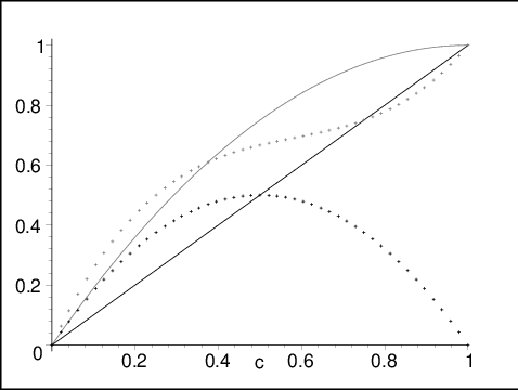
In particular, if m1⩽mm_{1}\leqslant m then λ0,1⩽λ1,0\lambda_{0,1}\leqslant\lambda_{1,0}. Assuming for a while that we are dealing with species of gases with same masses m=m1m=m_{1}, then in the true inelastic case (i.e., e<1e<1) one also has λ1,0>λ0,1\lambda_{1,0}>\lambda_{0,1}. This situation is very particular to inelastic scattering and means that the cooling process of the temperature happens more rapidly than the forcing of the momentum by the background, whereas when κ=1/2\kappa=1/2 these two processes happen at exactly the same speed (λ0,1=λ1,0)(\lambda_{0,1}=\lambda_{1,0}). Note also that, whenever λ0,1>λ1,0\lambda_{0,1}>\lambda_{1,0} (due to the ratio of mass different from 11), the smallest eigenvalue corresponds to the momentum relaxation and not the energy relaxation anymore. This contrasts very much with the linearized case (see [7]). Note also that the first eigenvalues are ordered as illustrated in Fig. 1.

The above result can be summarized in the following where the last statement follows from the fact that ℒ𝗆𝖺𝗑+Id\mathcal{L}_{\mathsf{max}}+\mbox{Id} is a self-adjoint compact operator of L2​(ℳ−1)L^{2}(\mathcal{M}^{-1}).

Theorem 3.2.

The operator −ℒ𝗆𝖺𝗑-\mathcal{L}_{\mathsf{max}} is a bounded self-adjoint positive operator of L2​(ℳ−1)L^{2}(\mathcal{M}^{-1}) whose spectrum is composed of an essential part {+1}\{+1\} plus the following discrete part:

𝔖p​(−ℒ𝗆𝖺𝗑)={λn,ℓ;n,ℓ∈ℕ}⊂[0,1)\mathfrak{S}_{p}(-\mathcal{L}_{\mathsf{max}})=\left\{\lambda_{n,\ell}\,;\,n,\,\ell\in\mathbb{N}\right\}\subset[0,1)

where λn,ℓ\lambda_{n,\ell} is given by (3.5). Moreover, λ0,0=0\lambda_{0,0}=0 is a simple eigenvalue of ℒ𝗆𝖺𝗑\mathcal{L}_{\mathsf{max}} associated to the eigenvector ℳ\mathcal{M} and −ℒ𝗆𝖺𝗑-\mathcal{L}_{\mathsf{max}} admits a positive spectral gap

μ𝗆𝖺𝗑=min⁡{λ1,0;λ0,1}=min⁡{κ;2​κ​(1−κ)}.\mu_{\mathsf{max}}=\min\{\lambda_{1,0};\lambda_{0,1}\}=\min\{\kappa;2\kappa(1-\kappa)\}.

Finally, there exists a Hilbert basis of L2​(ℳ−1)L^{2}(\mathcal{M}^{-1}) made of eigenvectors of −ℒ𝗆𝖺𝗑.-\mathcal{L}_{\mathsf{max}}.

Refer to caption
Figure 1. Evolution of λ0,1\lambda_{0,1} (black solid line), λ1,0\lambda_{1,0} (black dotted line), λ1,1\lambda_{1,1} (grey dotted line) and λ0,2\lambda_{0,2} (grey solid line) as functions of c∈[0,1]c\in[0,1]

3.2. Entropy estimate for Maxwell molecules

The result of the above section allows to provide a quantitative version of the HH-Theorem. Precisely, for any f∈L2​(ℳ−1)f\in L^{2}(\mathcal{M}^{-1}) orthogonal to ℳ\mathcal{M}, using the decomposition of both ℒ𝗆𝖺𝗑​f\mathcal{L}_{\mathsf{max}}f and ff on the Hilbert basis of L2​(ℳ−1)L^{2}(\mathcal{M}^{-1}) made of eigenvectors of −ℒ𝗆𝖺𝗑-\mathcal{L}_{\mathsf{max}} (see Theorem 3.2), it is easily proved that:

𝒟𝗆𝖺𝗑(f):=−∫ℝv3ℒ𝗆𝖺𝗑(f)fℳ−1dv⩾μ𝗆𝖺𝗑∥f∥L2​(ℳ−1)2,∀f⊥Span(ℳ).\mathcal{D}_{\mathsf{max}}(f):=-\int_{{\mathbb{R}}_{v}^{3}}\mathcal{L}_{\mathsf{max}}(f)\,f\,\mathcal{M}^{-1}\,\,\mathrm{d}{v}\geqslant\mu_{\mathsf{max}}\,\|f\|_{L^{2}(\mathcal{M}^{-1})}^{2},\qquad\forall f\bot\,\mathrm{Span}(\mathcal{M}). (3.7)

It is well-known that such a coercivity estimate allows to obtain an exponential relaxation rate to equilibrium for the solution to the space homogeneous Boltzmann equation. Namely, given f0​(v)∈L2​(ℝ3,ℳ−1​(v)​d​v)f_{0}({v})\in L^{2}({\mathbb{R}}^{3},\mathcal{M}^{-1}({v})\,\mathrm{d}{v}) with unit mass

∫ℝ3f0​(v)​𝑑v=1,\int_{{\mathbb{R}}^{3}}f_{0}(v)\,\mathrm{d}v=1,

let ftf_{t} be the unique solution of (1.1) with initial condition ft=0=f0.f_{t=0}=f_{0}. According to the conservation of mass, it is clear that (ft−ℳ)(f_{t}-\mathcal{M}) is orthogonal to ℳ\mathcal{M} (for the L2​(ℝv3,ℳ−1​(v)​d​v)L^{2}({\mathbb{R}}_{v}^{3},\mathcal{M}^{-1}({v})\,\mathrm{d}{v}) scalar product) and, within the entropy language:

dd​t​HΦ​(ft|ℳ)=−2​𝒟𝗆𝖺𝗑​(ft)⩽−2​μ𝗆𝖺𝗑​HΦ​(ft|ℳ)\frac{\,\mathrm{d}}{\,\mathrm{d}t}H_{\Phi}(f_{t}|\mathcal{M})=-2\mathcal{D}_{\mathsf{max}}(f_{t})\leqslant-2\mu_{\mathsf{max}}\,H_{\Phi}(f_{t}|\mathcal{M})

for Φ⁡(x)=(x−1)2\Phi(x)=(x-1)^{2} or equivalently,

(∫ℝ3(ft−ℳ)2​ℳ−1​𝑑v)1/2⩽(∫ℝ3(f0−ℳ)2​ℳ−1​𝑑v)1/2​exp⁡(−μ𝗆𝖺𝗑​t),∀t⩾0.\left(\int_{{\mathbb{R}}^{3}}(f_{t}-\mathcal{M})^{2}\,\mathcal{M}^{-1}\,\,\mathrm{d}{v}\right)^{1/2}\leqslant\left(\int_{{\mathbb{R}}^{3}}(f_{0}-\mathcal{M})^{2}\,\mathcal{M}^{-1}\,\,\mathrm{d}{v}\right)^{1/2}\,\exp\left(-\mu_{\mathsf{max}}t\right),\qquad\forall t\geqslant 0.

We obtain in this way an explicit exponential relaxation rate towards equilibrium for the solution to the space homogeneous linear Boltzmann equation which is valid for granular gases of Maxwell molecules and generalizes a well-known result for classical gases [11]. More interesting is the fact that the knowledge of the spectral gap of ℒ𝗆𝖺𝗑\mathcal{L}_{\mathsf{max}} allows to recover an explicit estimate of the spectral gap of the linear Boltzmann operator for hard-spheres ℒ𝗁𝗌\mathcal{L}_{\mathsf{hs}} through a suitable comparison of the entropy production functionals 𝒟𝗁𝗌\mathcal{D}_{{\mathsf{hs}}} and 𝒟𝗆𝖺𝗑\mathcal{D}_{{\mathsf{max}}}. This is the subject of the following section.

3.3. Entropy estimate for hard-spheres

The goal of this subsection is to show that the entropy production functional 𝒟𝗁𝗌\mathcal{D}_{{\mathsf{hs}}} for hard-spheres relates to the one for Maxwell molecules 𝒟𝗆𝖺𝗑\mathcal{D}_{\mathsf{max}}. More precisely we shall show that

Proposition 3.3.

The entropy production functionals 𝒟𝗁𝗌\mathcal{D}_{\mathsf{hs}} and 𝒟𝗆𝖺𝗑\mathcal{D}_{\mathsf{max}} are related by:

𝒟𝗁𝗌​(f)⩾C⋆​𝒟𝗆𝖺𝗑​(f),∀f∈𝒟⁡(ℒ𝗁𝗌)\mathcal{D}_{{\mathsf{hs}}}(f)\geqslant C^{\star}\,\mathcal{D}_{\mathsf{max}}(f),\qquad\forall f\in\mathscr{D}(\mathcal{L}_{\mathsf{hs}})

for some explicit constant C⋆C^{\star} depending only on α\alpha and β\beta.

Remark 3.4.

The idea of searching for such an inequality was already present in [2], but here the method of proof is different and simpler: one does not need any triangular inequality between collisions, and the proof reduces to a careful study of a convolution integral.

Remark 3.5.

Note that in the hard-spheres case, the operator ℒ𝗁𝗌\mathcal{L}_{\mathsf{hs}} is unbounded. For a careful study of its properties (compactness of the non-local part, definition of the associated C0C^{0}-semigroup of contraction in the Hilbert space L2​(ℳ−1)L^{2}(\mathcal{M}^{-1})) we refer to [1].

Proof.

Let f∈𝒟⁡(ℒ𝗁𝗌)f\in\mathscr{D}(\mathcal{L}_{\mathsf{hs}}). We set u1=0u_{1}=0 in this proof without restriction since this only amounts to a space translation.

We introduce the following parametrization, for fixed n∈𝕊2n\in{\mathbb{S}}^{2}, v=r​n+v¯{v}=rn+\bar{v}, v⋆=r⋆​n+v¯{v}^{\star}=r^{\star}n+\bar{v}, w=rw​n+w¯{w}=r_{w}n+\bar{w}, w⋆=rw⋆​n+w¯{w}^{\star}=r_{{w}^{\star}}n+\bar{w}, where r,r⋆,rwr,r^{\star},r_{w} and rw⋆r_{{w}^{\star}} are real numbers and v¯,w¯\bar{v},\bar{w} are orthogonal to nn. Simple computations show that

rw=r⋆2​α​(1−β)+(1−12​α​(1−β))​r,r_{w}=\frac{r^{\star}}{2\alpha(1-\beta)}+\left(1-\frac{1}{2\alpha(1-\beta)}\right)r,

while

rw⋆=(12​α​(1−β)−1−αα)​r⋆+(1α−12​α​(1−β))​r.r_{{w}^{\star}}=\left(\frac{1}{2\alpha(1-\beta)}-\frac{1-\alpha}{\alpha}\right)r^{\star}+\left(\frac{1}{\alpha}-\frac{1}{2\alpha(1-\beta)}\right)r.

Therefore, rwr_{w} and rw⋆r_{{w}^{\star}} only depend on rr and r⋆r^{\star}. Then if we denote θ\theta the angle between q~\widetilde{q} and nn, we get from Prop. 2.3, where we set g=fℳg=\frac{f}{\mathcal{M}},

𝒟𝗁𝗌​(f)=12​π​∫𝕊2∫r,r⋆∈ℝ∫v¯,w¯∈n⊥|q|​cos⁡θ​[g⁡(r⋆​n+v¯)−g⁡(r​n+v¯)]2ℳ1​(rw​n+w¯)​ℳ​(r​n+v¯)​d​v¯​d​w¯​d​r​d​r⋆​d​n\mathcal{D}_{{\mathsf{hs}}}(f)=\frac{1}{2\pi}\,\int_{{\mathbb{S}}^{2}}\int_{r,r^{\star}\in{\mathbb{R}}}\int_{\bar{v},\bar{w}\in n^{\bot}}|q|\,\cos\theta\,\Big[g(r^{\star}n+\bar{v})-g(rn+\bar{v})\Big]^{2}\\ \mathcal{M}_{1}(r_{w}n+\bar{w})\,\mathcal{M}(rn+\bar{v})\,\mathrm{d}\bar{v}\,\,\mathrm{d}\bar{w}\,\,\mathrm{d}r\,\,\mathrm{d}r^{\star}\,\,\mathrm{d}n

with

|q|=(|v¯−w¯|2+(2​κ)−2​|r⋆−r|2)1/2|q|=\Big(|\bar{v}-\bar{w}|^{2}+(2\kappa)^{-2}|r^{\star}-r|^{2}\Big)^{1/2}

and

cos⁡θ=(2​κ)−1​|r⋆−r|(|v¯−w¯|2+(2​κ)−2​|r⋆−r|2)1/2,\cos\theta=\frac{(2\kappa)^{-1}|r^{\star}-r|}{\left(|\bar{v}-\bar{w}|^{2}+(2\kappa)^{-2}|r^{\star}-r|^{2}\right)^{1/2}},

where we recall that κ=α⁡(1−β)\kappa=\alpha(1-\beta). We split the integral into two parts according to |r⋆−r|⩾ϱ0>0|r^{\star}-r|\geqslant\varrho_{0}>0 or |r⋆−r|⩽ϱ0|r^{\star}-r|\leqslant\varrho_{0} where ϱ0\varrho_{0} is a positive parameter to be determine latter. Using the fact that |q|⩾|r⋆−r|/2​κ|q|\geqslant|r^{\star}-r|/2\kappa, one has the following estimate for the first part of the integral

12​π∫𝕊2dn∫{|r⋆−r|⩾ϱ0}drdr⋆∫v¯,w¯∈n⊥|q|cosθℳ(rn+v¯)ℳ1(rwn+w¯)[g⁡(r⋆​n+v¯)−g⁡(r​n+v¯)]2​d​v¯​d​w¯⩾(2​κ)−1​ϱ02​π∫𝕊2dn∫{|r⋆−r|⩾ϱ0}drdr⋆∫v¯,w¯∈n⊥cos⁡θ​ℳ​(r​n+v¯)​ℳ1​(rw​n+w¯)​[g⁡(r⋆​n+v¯)−g⁡(r​n+v¯)]2​dv¯​dw¯\begin{split}\frac{1}{2\pi}\,&\int_{{\mathbb{S}}^{2}}\,\mathrm{d}n\int_{\{|r^{\star}-r|\geqslant\varrho_{0}\}}\,\mathrm{d}r\,\,\mathrm{d}r^{\star}\int_{\bar{v},\bar{w}\in n^{\bot}}|q|\,\cos\theta\,\mathcal{M}(rn+\bar{v})\,\mathcal{M}_{1}(r_{w}n+\bar{w})\\ &\phantom{+++++++++++++}\Big[g(r^{\star}n+\bar{v})-g(rn+\bar{v})\Big]^{2}\,\,\mathrm{d}\bar{v}\,\,\mathrm{d}\bar{w}\\ &\geqslant\frac{(2\kappa)^{-1}\,\varrho_{0}}{2\pi}\,\int_{{\mathbb{S}}^{2}}\,\mathrm{d}n\int_{\{|r^{\star}-r|\geqslant\varrho_{0}\}}\,\,\mathrm{d}r\,\,\mathrm{d}r^{\star}\\ &\int_{\bar{v},\bar{w}\in n^{\bot}}\cos\theta\,\mathcal{M}(rn+\bar{v})\,\mathcal{M}_{1}(r_{w}n+\bar{w})\Big[g(r^{\star}n+\bar{v})-g(rn+\bar{v})\Big]^{2}\,\,\mathrm{d}\bar{v}\,\,\mathrm{d}\bar{w}\end{split}

which corresponds (up to the multiplicative factor (2​κ)−1​ϱ0(2\kappa)^{-1}\,\varrho_{0}) to the integral for |r−r⋆|⩾ϱ0|r-r^{\star}|\geqslant\varrho_{0} corresponding to Maxwell molecules, i.e.,

−∫ℝ3χ{|r−r⋆|⩾ϱ0}ℒ𝗁𝗌(f)fℳ−1dv⩾−ϱ02​κ∫ℝ3χ{|r−r⋆|⩾ϱ0}ℒ𝗆𝖺𝗑(f)fℳ−1dv.-\int_{{\mathbb{R}}^{3}}\chi_{\{|r-r^{\star}|\geqslant\varrho_{0}\}}\mathcal{L}_{\mathsf{hs}}(f)f\mathcal{M}^{-1}\,\mathrm{d}{v}\geqslant-\frac{\varrho_{0}}{2\kappa}\int_{{\mathbb{R}}^{3}}\chi_{\{|r-r^{\star}|\geqslant\varrho_{0}\}}\mathcal{L}_{\mathsf{max}}(f)f\mathcal{M}^{-1}\,\mathrm{d}{v}. (3.8)

Concerning now the second part of the integral (corresponding to |r⋆−r|⩽ϱ0|r^{\star}-r|\leqslant\varrho_{0}), we use that |q|⩾|v¯−w¯||q|\geqslant|\bar{v}-\bar{w}| and we isolate the integration over w¯\bar{w}:

−∫ℝ3χ{|r−r⋆|⩽ϱ0}ℒ𝗁𝗌(f)fℳ−1dv⩾12​π∫𝕊2dn∫{|r⋆−r|⩽ϱ0}drdr⋆|r⋆−r|∫v¯∈n⊥(2κ)−1(m12​π​Θ1)−3/2(∫w¯∈n⊥|v¯−w¯|​ℳ1​(w¯)(|v¯−w¯|2+(2​κ)−2​|r⋆−r|2)1/2dw¯)ℳ⁡(r​n+v¯)​ℳ1​(rw​n)​[g⁡(r⋆​n+v¯)−g⁡(r​n+v¯)]2​d​v¯\begin{split}-\int_{{\mathbb{R}}^{3}}\,&\chi_{\{|r-r^{\star}|\leqslant\varrho_{0}\}}\mathcal{L}_{\mathsf{hs}}(f)f\mathcal{M}^{-1}\,\mathrm{d}{v}\geqslant\frac{1}{2\pi}\,\int_{{\mathbb{S}}^{2}}\,\mathrm{d}n\int_{\{|r^{\star}-r|\leqslant\varrho_{0}\}}\,\mathrm{d}r\,\,\mathrm{d}r^{\star}\,|r^{\star}-r|\\ &\int_{\bar{v}\in n^{\bot}}(2\kappa)^{-1}\left(\frac{m_{1}}{2\pi\Theta_{1}}\right)^{-3/2}\left(\int_{\bar{w}\in n^{\bot}}\frac{|\bar{v}-\bar{w}|\,\mathcal{M}_{1}(\bar{w})}{\left(|\bar{v}-\bar{w}|^{2}+(2\kappa)^{-2}|r^{\star}-r|^{2}\right)^{1/2}}\,\,\mathrm{d}\bar{w}\right)\\ &\phantom{+++++}\mathcal{M}(rn+\bar{v})\,\mathcal{M}_{1}(r_{w}n)\,\Big[g(r^{\star}n+\bar{v})-g(rn+\bar{v})\Big]^{2}\,\,\mathrm{d}\bar{v}\end{split}

where we used the fact that, since w¯\bar{w} is orthogonal to nn,

ℳ1(rwn+w¯)=(m12​π​Θ1)−3/2ℳ1(w¯)ℳ1(rwn).\mathcal{M}_{1}(r_{w}n+\bar{w})=\left(\frac{m_{1}}{2\pi\Theta_{1}}\right)^{-3/2}\mathcal{M}_{1}(\bar{w})\mathcal{M}_{1}(r_{w}n).

Setting ξ=|r⋆−r|/2​κ\xi=|r^{\star}-r|/2\kappa, if one were able to prove that there is a constant CC such that

∫ℝ2|v¯−w¯|​ℳ1​(w¯)(|v¯−w¯|2+ξ2)1/2​𝑑w¯⩾C​∫ℝ2ℳ1​(w¯)(|v¯−w¯|2+ξ2)1/2​𝑑w¯\int_{{\mathbb{R}}^{2}}\frac{|\bar{v}-\bar{w}|\,\mathcal{M}_{1}(\bar{w})}{\left(|\bar{v}-\bar{w}|^{2}+\xi^{2}\right)^{1/2}}\,\,\mathrm{d}\bar{w}\geqslant C\,\int_{{\mathbb{R}}^{2}}\frac{\mathcal{M}_{1}(\bar{w})}{\left(|\bar{v}-\bar{w}|^{2}+\xi^{2}\right)^{1/2}}\,\,\mathrm{d}\bar{w} (3.9)

uniformly for v¯∈ℝ2\bar{v}\in{\mathbb{R}}^{2} and ξ∈[0,ϱ0/2​κ]\xi\in[0,\varrho_{0}/2\kappa], then one would obtain the desired estimate (by doing all the previous transformations backward):

−∫ℝ3χ{|r−r⋆|⩽ϱ0}ℒ𝗁𝗌(f)fℳ−1dv⩾−C∫ℝ3χ{|r−r⋆|⩽ϱ0}ℒ𝗆𝖺𝗑(f)fℳ−1dv.-\int_{{\mathbb{R}}^{3}}\chi_{\{|r-r^{\star}|\leqslant\varrho_{0}\}}\mathcal{L}_{\mathsf{hs}}(f)f\mathcal{M}^{-1}\,\mathrm{d}{v}\geqslant-C\int_{{\mathbb{R}}^{3}}\chi_{\{|r-r^{\star}|\leqslant\varrho_{0}\}}\mathcal{L}_{\mathsf{max}}(f)f\mathcal{M}^{-1}\,\mathrm{d}{v}.

To study the convolution integral of (3.9), we make a second splitting between |w¯−v¯|⩾ϱ1>0|\bar{w}-\bar{v}|\geqslant\varrho_{1}>0 and |w¯−v¯|⩽ϱ1|\bar{w}-\bar{v}|\leqslant\varrho_{1} (for some ϱ1>0\varrho_{1}>0). It gives

∫w¯∈ℝ2|v¯−w¯|​ℳ1​(w¯)(|v¯−w¯|2+ξ2)1/2​dw¯⩾∫{|w¯−v¯|⩾ϱ1}|v¯−w¯|​ℳ1​(w¯)(|v¯−w¯|2+ξ2)1/2dw¯⩾ϱ1∫{|w¯−v¯|⩾ϱ1}ℳ1​(w¯)(|v¯−w¯|2+ξ2)1/2dw¯⩾ϱ1(∫ℝ2ℳ1​(w¯)(|v¯−w¯|2+ξ2)1/2dw¯−∫{|w¯−v¯|⩽ϱ1}ℳ1​(w¯)(|v¯−w¯|2+ξ2)1/2dw¯).\int_{\bar{w}\in{\mathbb{R}}^{2}}\frac{|\bar{v}-\bar{w}|\,\mathcal{M}_{1}(\bar{w})}{\left(|\bar{v}-\bar{w}|^{2}+\xi^{2}\right)^{1/2}}\,\,\mathrm{d}\bar{w}\\ \geqslant\int_{\{|\bar{w}-\bar{v}|\geqslant\varrho_{1}\}}\frac{|\bar{v}-\bar{w}|\,\mathcal{M}_{1}(\bar{w})}{\left(|\bar{v}-\bar{w}|^{2}+\xi^{2}\right)^{1/2}}\,\,\mathrm{d}\bar{w}\geqslant\varrho_{1}\,\int_{\{|\bar{w}-\bar{v}|\geqslant\varrho_{1}\}}\frac{\mathcal{M}_{1}(\bar{w})}{\left(|\bar{v}-\bar{w}|^{2}+\xi^{2}\right)^{1/2}}\,\,\mathrm{d}\bar{w}\\ \geqslant\varrho_{1}\,\Bigg(\int_{{\mathbb{R}}^{2}}\frac{\mathcal{M}_{1}(\bar{w})}{\left(|\bar{v}-\bar{w}|^{2}+\xi^{2}\right)^{1/2}}\,\,\mathrm{d}\bar{w}-\int_{\{|\bar{w}-\bar{v}|\leqslant\varrho_{1}\}}\frac{\mathcal{M}_{1}(\bar{w})}{\left(|\bar{v}-\bar{w}|^{2}+\xi^{2}\right)^{1/2}}\,\,\mathrm{d}\bar{w}\Bigg).

Then we use the obvious estimates

∀v¯∈ℝ2,∀ξ∈[0,ϱ0/2​κ],∫ℝ2ℳ1​(w¯)(|v¯−w¯|2+ξ2)1/2​𝑑w¯⩾C⁡(κ,ϱ0)1+|v¯|\forall\,\bar{v}\in{\mathbb{R}}^{2},\ \forall\,\xi\in[0,\varrho_{0}/2\kappa],\int_{{\mathbb{R}}^{2}}\frac{\mathcal{M}_{1}(\bar{w})}{\left(|\bar{v}-\bar{w}|^{2}+\xi^{2}\right)^{1/2}}\,\,\mathrm{d}\bar{w}\geqslant\frac{C(\kappa,\varrho_{0})}{1+|\bar{v}|}

for an explicit constant C⁡(κ,ϱ0)>0C(\kappa,\varrho_{0})>0 depending only on κ,ϱ0\kappa,\varrho_{0}, and

∀v¯∈ℝ2,∀ξ∈[0,ϱ0/2κ],∫{|w¯−v¯|⩽ϱ1}ℳ1​(w¯)(|v¯−w¯|2+ξ2)1/2dw¯⩽C(κ,ϱ1)e−|v¯|2.\forall\,\bar{v}\in{\mathbb{R}}^{2},\ \forall\,\xi\in[0,\varrho_{0}/2\kappa],\int_{\{|\bar{w}-\bar{v}|\leqslant\varrho_{1}\}}\frac{\mathcal{M}_{1}(\bar{w})}{\left(|\bar{v}-\bar{w}|^{2}+\xi^{2}\right)^{1/2}}\,\,\mathrm{d}\bar{w}\leqslant C(\kappa,\varrho_{1})\,e^{-|\bar{v}|^{2}}.

for an explicit constant C⁡(κ,ϱ1)>0C(\kappa,\varrho_{1})>0 going to 00 as ϱ1\varrho_{1} goes to 00. It yields for ϱ1\varrho_{1} small enough (depending on ϱ0\varrho_{0})

∫{|w¯−v¯|⩽ϱ1}ℳ1​(w¯)(|v¯−w¯|2+ξ2)1/2dw¯⩽12∫ℝ2ℳ1​(w¯)(|v¯−w¯|2+ξ2)1/2dw¯.\int_{\{|\bar{w}-\bar{v}|\leqslant\varrho_{1}\}}\frac{\mathcal{M}_{1}(\bar{w})}{\left(|\bar{v}-\bar{w}|^{2}+\xi^{2}\right)^{1/2}}\,\,\mathrm{d}\bar{w}\leqslant\frac{1}{2}\,\int_{{\mathbb{R}}^{2}}\frac{\mathcal{M}_{1}(\bar{w})}{\left(|\bar{v}-\bar{w}|^{2}+\xi^{2}\right)^{1/2}}\,\,\mathrm{d}\bar{w}. (3.10)

for any v¯∈ℝ2,ξ∈[0,ϱ0/2​κ]\bar{v}\in{\mathbb{R}}^{2},\xi\in[0,\varrho_{0}/2\kappa] (we also refer to the Appendix A of this paper for a construction of the parameter ϱ1\varrho_{1}). Consequently, for this choice of ϱ1\varrho_{1} we obtain (3.9) with C=ϱ1/2C=\varrho_{1}/2, i.e.,

−∫ℝ3χ{|r−r⋆|⩽ϱ0}ℒ𝗁𝗌(f)fℳ−1dv⩾−ϱ12∫ℝ3χ{|r−r⋆|⩽ϱ0}ℒ𝗆𝖺𝗑(f)fℳ−1dv.-\int_{{\mathbb{R}}^{3}}\chi_{\{|r-r^{\star}|\leqslant\varrho_{0}\}}\mathcal{L}_{\mathsf{hs}}(f)f\mathcal{M}^{-1}\,\mathrm{d}{v}\geqslant-\frac{\varrho_{1}}{2}\int_{{\mathbb{R}}^{3}}\chi_{\{|r-r^{\star}|\leqslant\varrho_{0}\}}\mathcal{L}_{\mathsf{max}}(f)f\mathcal{M}^{-1}\,\mathrm{d}{v}.

This, together with estimate (3.8), yield

𝒟𝗁𝗌​(f)⩾min⁡{ϱ02​κ,ϱ12}​𝒟𝗆𝖺𝗑​(f)\mathcal{D}_{{\mathsf{hs}}}(f)\geqslant\min\left\{\frac{\varrho_{0}}{2\kappa},\frac{\varrho_{1}}{2}\right\}\,\mathcal{D}_{\mathsf{max}}(f)

which concludes the proof. ∎

Remark 3.6.

The constant C⋆C^{\star} from the proof can be optimized according to the parameter ϱ0\varrho_{0}, by expliciting ϱ1\varrho_{1} as a function of ϱ0\varrho_{0}. Precisely, making use of Lemma A.1 given in the Appendix,

C⋆=min⁡{ϱ02​κ,ϱ12}⩾η5C^{\star}=\min\left\{\frac{\varrho_{0}}{2\kappa},\frac{\varrho_{1}}{2}\right\}\geqslant\dfrac{\eta}{\sqrt{5}}

with η=2​Θ1m1​erf−1​(12)\eta=\sqrt{\frac{2\Theta_{1}}{m_{1}}}\,\mathrm{erf}^{-1}\left(\frac{1}{2}\right) where erf−1\mathrm{erf}^{-1} denotes the inverse error function, erf−1​(12)≃0.4769.\mathrm{erf}^{-1}(\frac{1}{2})\simeq 0.4769. Notice that this lower bound for C⋆C^{\star} does not depend on the parameters α,β\alpha,\beta.

Remark 3.7.

The above Proposition provides an estimate of the spectral gap of ℒ𝗁𝗌\mathcal{L}_{\mathsf{hs}} in L2​(ℳ−1)L^{2}(\mathcal{M}^{-1}). Precisely, we recall from [1] that the spectrum of ℒ𝗁𝗌\mathcal{L}_{\mathsf{hs}} is made of continuous (essential) spectrum {λ∈ℝ;λ⩽−ν0}\{\lambda\in\mathbb{R}\,;\,\lambda\leqslant-\nu_{0}\} where ν0=infv∈ℝ3σ𝗁𝗌​(v)>0\nu_{0}=\inf_{{v}\in{\mathbb{R}}^{3}}\sigma_{\mathsf{hs}}({v})>0 and a decreasing sequence of real eigenvalues with finite algebraic multiplicities which unique possible cluster point is −ν0-\nu_{0}. Then, since 00 is an eigenvalue of ℒ𝗁𝗌\mathcal{L}_{\mathsf{hs}} associated to ℳ\mathcal{M}, one sees from the above Proposition that the spectral gap μ𝗁𝗌\mu_{\mathsf{hs}} of ℒ𝗁𝗌\mathcal{L}_{\mathsf{hs}} satisfies

μ𝗁𝗌:=min{λ:−λ∈(−ν0,0),−λ∈𝔖(ℒ𝗁𝗌)∖{0}}⩾C⋆μ𝗆𝖺𝗑⩾η​min⁡{κ,2​κ​(1−κ)}5.\mu_{\mathsf{hs}}:=\min\bigg\{\lambda:-\lambda\in(-\nu_{0},0),-\lambda\in\mathfrak{S}(\mathcal{L}_{\mathsf{hs}})\setminus\{0\}\bigg\}\geqslant C^{\star}\mu_{\mathsf{max}}\geqslant\frac{\eta\min\{\kappa,2\kappa(1-\kappa)\}}{\sqrt{5}}.

To summarize, one gets the following coercivity estimate for the Dirichlet form:

Theorem 3.8.

For 𝒬=ℒ𝗁𝗌\mathcal{Q}=\mathcal{L}_{\mathsf{hs}} or ℒ𝗆𝖺𝗑\mathcal{L}_{\mathsf{max}}, one has the following:

−∫ℝ3𝒬(f)(v)f(v)ℳ−1(v)dv⩾μ∥f−ϱfℳ∥L2​(ℳ−1)2,∀f∈𝒟(𝒬)-\int_{{\mathbb{R}}^{3}}\mathcal{Q}(f)({v})f({v})\mathcal{M}^{-1}({v})\,\mathrm{d}{v}\geqslant\mu\|f-\varrho_{f}\mathcal{M}\|_{L^{2}(\mathcal{M}^{-1})}^{2},\qquad\forall f\in\mathscr{D}(\mathcal{Q})

where, ϱf=∫ℝ3f⁡(v)​𝑑v,\varrho_{f}=\displaystyle\int_{{\mathbb{R}}^{3}}f({v})\,\mathrm{d}{v}, and μ=μ𝗆𝖺𝗑\mu=\mu_{\mathsf{max}} whenever 𝒬=ℒ𝗆𝖺𝗑\mathcal{Q}=\mathcal{L}_{\mathsf{max}} while, for hard-spheres interactions, i.e., 𝒬=ℒ𝗁𝗌\mathcal{Q}=\mathcal{L}_{\mathsf{hs}}, one has μ⩾C⋆​μ𝗆𝖺𝗑\mu\geqslant C^{\star}\mu_{\mathsf{max}}.

Proof.

If ϱf=0\varrho_{f}=0, the proof follows directly from Proposition 3.3 and (3.7). Now, if ff is a given function with non-zero mean ϱf\varrho_{f}, set h=f−ϱf​ℳh=f-\varrho_{f}\mathcal{M}. Then, ϱh=0\varrho_{h}=0 so that

−∫ℝ3𝒬(h)(v)h(v)ℳ−1(v)dv⩾μ∥h∥L2​(ℳ−1)2.-\int_{{\mathbb{R}}^{3}}\mathcal{Q}(h)({v})h({v})\mathcal{M}^{-1}({v})\,\mathrm{d}{v}\geqslant\mu\|h\|_{L^{2}(\mathcal{M}^{-1})}^{2}.

This leads to the result since 𝒬⁡(h)=𝒬⁡(f)\mathcal{Q}(h)=\mathcal{Q}(f) and ∫ℝ3𝒬⁡(f)​𝑑v=0\displaystyle\int_{{\mathbb{R}}^{3}}\mathcal{Q}(f)\,\mathrm{d}{v}=0. ∎

Adopting now the entropy language, one obtains the following relaxation rate, which is also new in the context of linear Boltzmann equation:

Corollary 3.9.

Let f0​(v)∈L2​(ℝv3,ℳ−1​(v)​d​v)f_{0}({v})\in L^{2}({\mathbb{R}}_{v}^{3},\mathcal{M}^{-1}({v})\,\mathrm{d}{v}) be given and let f⁡(t)f(t) be the unique solution of (1.1) with initial condition f⁡(t=0)=f0.f(t=0)=f_{0}. Then, for any t⩾0,t\geqslant 0, one has the following

‖f⁡(t)−ℳ‖L2​(ℳ−1)⩽exp⁡(−μ​t)​‖f0−ℳ‖L2​(ℳ−1),∀t⩾0,\left\|f(t)-\mathcal{M}\right\|_{L^{2}(\mathcal{M}^{-1})}\leqslant\exp(-\mu t)\left\|f_{0}-\mathcal{M}\right\|_{L^{2}(\mathcal{M}^{-1})},\qquad\forall t\geqslant 0,

where μ=μ𝗆𝖺𝗑\mu=\mu_{\mathsf{max}} when 𝒬=𝒬𝗆𝖺𝗑\mathcal{Q}=\mathcal{Q}_{\mathsf{max}} while, for hard-spheres interactions, i.e., 𝒬=𝒬𝗁𝗌\mathcal{Q}=\mathcal{Q}_{\mathsf{hs}}, one has μ⩾C⋆​μ𝗆𝖺𝗑\mu\geqslant C^{\star}\mu_{\mathsf{max}}.

We state another corollary of the above Theorem 3.8 in which we strengthen the coercivity estimate:

Corollary 3.10.

For 𝒬=ℒ𝗁𝗌\mathcal{Q}=\mathcal{L}_{\mathsf{hs}} or ℒ𝗆𝖺𝗑\mathcal{L}_{\mathsf{max}}, there exists cσ>0c_{\sigma}>0 such that

−∫ℝ3𝒬(f)(v)f(v)ℳ−1(v)dv⩾cσ∥(f−ϱfℳ)σ∥L2​(ℳ−1)2∀f∈𝒟(𝒬)-\int_{{\mathbb{R}}^{3}}\mathcal{Q}(f)({v})f({v})\mathcal{M}^{-1}({v})\,\mathrm{d}{v}\geqslant c_{\sigma}\|(f-\varrho_{f}\mathcal{M})\sqrt{\sigma}\|_{L^{2}(\mathcal{M}^{-1})}^{2}\qquad\qquad\forall f\in\mathscr{D}(\mathcal{Q})

where, ϱf=∫ℝ3f⁡(v)​𝑑v\varrho_{f}=\displaystyle\int_{{\mathbb{R}}^{3}}f({v})\,\mathrm{d}{v} and σ⁡(v)\sigma(v) is the collision frequency associated to 𝒬\mathcal{Q}.

Proof.

If 𝒬=ℒ𝗆𝖺𝗑\mathcal{Q}=\mathcal{L}_{\mathsf{max}}, since σ𝗆𝖺𝗑​(v)=1\sigma_{\mathsf{max}}(v)=1 the estimate is nothing but Theorem 3.8. Let us consider now the hard-spheres case, 𝒬=ℒ𝗁𝗌.\mathcal{Q}=\mathcal{L}_{\mathsf{hs}}. Arguing as in the proof of Theorem 3.8, it suffices to prove the result for f⊥ℳf\bot\,\mathcal{M}, i.e., whenever ϱf=0\varrho_{f}=0. We recall from [1] that ℒ𝗁𝗌\mathcal{L}_{\mathsf{hs}} splits as

ℒ𝗁𝗌​f=𝒦​f−σ𝗁𝗌​f,f∈𝒟⁡(ℒ𝗁𝗌)\mathcal{L}_{\mathsf{hs}}f=\mathscr{K}f-\sigma_{\mathsf{hs}}f,\quad f\in\mathscr{D}(\mathcal{L}_{\mathsf{hs}})

where 𝒦\mathscr{K} is a bounded (and compact) operator in L2​(ℳ−1)L^{2}(\mathcal{M}^{-1}). We then have

‖f​σ𝗁𝗌‖L2​(ℳ−1)2=∫ℝv3𝒦⁡(f)​f​ℳ−1​𝑑v−∫ℝv3ℒ𝗁𝗌​(f)​f​ℳ−1​𝑑v⩽‖𝒦‖​‖f‖L2​(ℳ−1)2+𝒟𝗁𝗌​(f)⩽(‖𝒦‖μ𝗆𝖺𝗑​C⋆+1)​𝒟𝗁𝗌​(f)\begin{split}\|f\sqrt{\sigma_{\mathsf{hs}}}\|^{2}_{L^{2}(\mathcal{M}^{-1})}&=\int_{{\mathbb{R}}^{3}_{v}}\mathscr{K}(f)\,f\,\mathcal{M}^{-1}\,\mathrm{d}{v}-\int_{{\mathbb{R}}^{3}_{v}}\mathcal{L}_{\mathsf{hs}}(f)\,f\,\mathcal{M}^{-1}\,\mathrm{d}{v}\\ &\leqslant\|\mathscr{K}\|\|f\|^{2}_{L^{2}(\mathcal{M}^{-1})}+\mathscr{D}_{\mathsf{hs}}(f)\leqslant\bigg(\frac{\|\mathscr{K}\|}{\mu_{\mathsf{max}}C^{\star}}+1\bigg)\mathscr{D}_{\mathsf{hs}}(f)\end{split}

where ‖𝒦‖\|\mathscr{K}\| stands for the norm of 𝒦\mathscr{K} as a bounded operator on L2​(ℳ−1)L^{2}(\mathcal{M}^{-1}) and we used Theorem 3.8. The corollary follows with

cσ=C⋆​μ𝗆𝖺𝗑‖𝒦‖+C⋆​μ𝗆𝖺𝗑.c_{\sigma}=\frac{C^{\star}\mu_{\mathsf{max}}}{\|\mathscr{K}\|+C^{\star}\mu_{\mathsf{max}}}.

∎

Remark 3.11.

Here again, as in Prop. 3.3, the constant cσ>0c_{\sigma}>0 can be quantitatively estimated using for instance the estimate‖𝒦‖⩽2​π(1+τ)2​π​Θ1m1\|\mathscr{K}\|\leqslant\frac{2\pi}{(1+\tau)^{2}}\sqrt{\frac{\pi\Theta_{1}}{m_{1}}} that can be deduced without major difficulty from the explicit expression of 𝒦\mathscr{K} provided in [1] with τ=(1−2​κ)/κ>0\tau=(1-2\kappa)/\kappa>0.

Remark 3.12.

Recalling that σ𝗁𝗌\sigma_{\mathsf{hs}} behaves like (1+|v|)(1+|v|), the above corollary allows to control from below the entropy production functional by the weighted L2​((1+|v|)​ℳ−1,d​v)L^{2}((1+|v|)\mathcal{M}^{-1},\,\mathrm{d}{v}) norm. Such a weighted estimate shall be very useful for the diffusion approximation.

4. Diffusion Approximation

We shall assume again in this whole section that u1=0u_{1}=0. From the results of the previous section, it is possible to derive some exact convergence results for the solution of the re-scaled linear kinetic Boltzmann equation

ε​∂tfε​(t,x,v)+v⋅∇xfε​(t,x,v)=1ε​𝒬​(fε)​(t,x,v),\varepsilon\partial_{t}f_{\varepsilon}(t,x,{v})+v\cdot\nabla_{x}f_{\varepsilon}(t,x,{v})=\dfrac{1}{\varepsilon}\mathcal{Q}(f_{\varepsilon})(t,x,{v}), (4.1)

with initial condition fε​(x,v,0)=f0​(x,v)⩾0f_{\varepsilon}(x,{v},0)=f_{0}(x,{v})\geqslant 0, with (x,v)∈ℝ3×ℝ3(x,v)\in{\mathbb{R}}^{3}\times{\mathbb{R}}^{3}. Note that all the analysis we perform here is also valid if the spatial domain denotes the three-dimensional torus 𝕋x3\mathbb{T}^{3}_{x}. One shall prove that fεf_{\varepsilon} converges, as ε→0\varepsilon\to 0, to ℳ⁡(v)​ϱ\mathcal{M}(v)\varrho where ϱ=ϱ⁡(t,x)\varrho=\varrho(t,x) is the solution to the (parabolic) diffusion equation:

{∂tϱ(t,x)=∇x⋅(𝖣∇xϱ(t,x)+u1ρ),t⩾0,x∈ℝ3,ϱ⁡(0,x)=ϱ0​(x)=∫ℝv3f0​(x,v)​𝑑v\begin{cases}\partial_{t}\varrho(t,x)=\nabla_{x}\cdot\left(\mathsf{D}\nabla_{x}\varrho(t,x)+u_{1}\,\rho\right),\qquad\qquad t\geqslant 0,\>x\in{\mathbb{R}}^{3},\\ \varrho(0,x)=\varrho_{0}(x)=\displaystyle\int_{{\mathbb{R}}_{v}^{3}}f_{0}(x,{v})\,\mathrm{d}{v}\end{cases} (4.2)

where the diffusion coefficient 𝖣\mathsf{D} depends on the model we investigate (hard-sphere interactions or Maxwell molecules). One shall adopt here the strategy of [12, 14]. Namely, to prove the convergence of the solution to (4.1) towards the solution ϱ\varrho of (4.2), the idea is to use the a priori estimate given by the production of entropy, as in [14] where this idea was applied to discrete velocity models of the Boltzmann equation. Let us define the number density and the current vector

ϱε​(t,x)=∫ℝv3fε​(t,x,v)​𝑑v,jε​(t,x)=1ε​∫ℝv3fε​(t,x,v)​v​𝑑v.\varrho_{\varepsilon}(t,x)=\int_{{\mathbb{R}}_{v}^{3}}f_{\varepsilon}(t,x,{v})\,\mathrm{d}{v},\qquad j_{\varepsilon}(t,x)=\frac{1}{\varepsilon}\,\int_{{\mathbb{R}}_{v}^{3}}f_{\varepsilon}(t,x,{v})\,v\,\,\,\mathrm{d}{v}.

We also define hεh_{\varepsilon} as

hε​(t,x,v)=1ε​(fε​(t,x,v)−ϱε​(t,x)​ℳ​(v)).h_{\varepsilon}(t,x,{v})=\dfrac{1}{\varepsilon}\bigg(f_{\varepsilon}(t,x,{v})-\varrho_{\varepsilon}(t,x)\mathcal{M}({v})\bigg).

Integrating (4.1) with respect to xx and v{v} and using the fact that the mean of 𝒬⁡(fε)\mathcal{Q}(f_{\varepsilon}) is zero, one gets the mass conservation identity

∫ℝx3×ℝv3fε​(x,v,t)​𝑑x​𝑑v=∫ℝx3×ℝv3f0​(x,v)​𝑑x​𝑑v,\int_{{\mathbb{R}}^{3}_{x}\times{\mathbb{R}}_{v}^{3}}f_{\varepsilon}(x,{v},t)\,\mathrm{d}x\,\mathrm{d}{v}=\int_{{\mathbb{R}}^{3}_{x}\times{\mathbb{R}}_{v}^{3}}f_{0}(x,{v})\,\mathrm{d}x\,\mathrm{d}{v}, (4.3)

which means (using the fact that the equation preserves non-negativity) that, for any T>0T>0, the sequence ϱε​(x,t)\varrho_{\varepsilon}(x,t) is bounded in L∞​(0,T,L1​(ℝx3)).L^{\infty}(0,T;L^{1}({\mathbb{R}}^{3}_{x})). Now, multiplying (4.1) by fε​ℳ−1f_{\varepsilon}\mathcal{M}^{-1} and integrating over ℝx3×ℝv3{\mathbb{R}}^{3}_{x}\times{\mathbb{R}}_{v}^{3}, we get

12​dd​t​∫ℝx3×ℝv3fε 2​(t,x,v)​ℳ−1​(v)​𝑑x​𝑑v+12​ε​∫ℝx3×ℝv3divx​(v​fε 2​(t,x,v))​ℳ−1​(v)​𝑑x​𝑑v−1ε2∫ℝx3×ℝv3fε𝒬(fε)ℳ−1dxdv=0.\dfrac{1}{2}\dfrac{\,\mathrm{d}}{\,\mathrm{d}t}\int_{{\mathbb{R}}^{3}_{x}\times{\mathbb{R}}_{v}^{3}}f^{\,2}_{\varepsilon}(t,x,{v})\mathcal{M}^{-1}({v})\,\mathrm{d}x\,\mathrm{d}{v}+\dfrac{1}{2\varepsilon}\int_{{\mathbb{R}}^{3}_{x}\times{\mathbb{R}}_{v}^{3}}\mathrm{div}_{x}\left({v}f^{\,2}_{\varepsilon}(t,x,{v})\right)\mathcal{M}^{-1}({v})\,\mathrm{d}x\,\mathrm{d}{v}\\ -\dfrac{1}{\varepsilon^{2}}\int_{{\mathbb{R}}^{3}_{x}\times{\mathbb{R}}_{v}^{3}}f_{\varepsilon}\,\mathcal{Q}(f_{\varepsilon})\mathcal{M}^{-1}\,\mathrm{d}x\,\mathrm{d}{v}=0. (4.4)

Now, because of the divergence form of the integrand, one sees that the second term in (4.4) is zero while, because of Corollary 3.10,

−1ε2​∫ℝx3×ℝv3fε​𝒬​(fε)​ℳ−1​𝑑x​𝑑v⩾cσε2∫ℝx3∥fε(t,x,⋅)−ϱε(t,x)ℳ∥L2​(ℝv3,σ⁡(v)​ℳ−1​(v)​d​v)2dx=cσ​∫ℝx3×ℝv3hε 2​(t,x,v)​ℳ−1​(v)​σ​(v)​dx​dv.\begin{split}-&\dfrac{1}{\varepsilon^{2}}\int_{{\mathbb{R}}^{3}_{x}\times{\mathbb{R}}_{v}^{3}}f_{\varepsilon}\,\mathcal{Q}(f_{\varepsilon})\mathcal{M}^{-1}\,\mathrm{d}x\,\mathrm{d}{v}\\ &\geqslant\dfrac{c_{\sigma}}{\varepsilon^{2}}\int_{{\mathbb{R}}^{3}_{x}}\|f_{\varepsilon}(t,x,\cdot)-\varrho_{\varepsilon}(t,x)\mathcal{M}\|_{L^{2}({\mathbb{R}}_{v}^{3},\sigma(v)\mathcal{M}^{-1}(v)\,\mathrm{d}v)}^{2}\,\mathrm{d}x\\ &=c_{\sigma}\int_{{\mathbb{R}}^{3}_{x}\times{\mathbb{R}}_{v}^{3}}h^{\,2}_{\varepsilon}(t,x,{v})\mathcal{M}^{-1}({v})\sigma(v)\,\mathrm{d}x\,\mathrm{d}{v}.\end{split} (4.5)

Consequently, Eq. (4.4), together with (4.5), leads to

12dd​t∫ℝx3×ℝv3fε2(x,v,t)ℳ−1(v)dxdv⩽−cσ∫ℝx3×ℝv3hε2(x,v,t)σ(v)ℳ−1(v)dxdv.\dfrac{1}{2}\dfrac{\,\mathrm{d}}{\,\mathrm{d}t}\int_{{\mathbb{R}}^{3}_{x}\times{\mathbb{R}}_{v}^{3}}f^{2}_{\varepsilon}(x,{v},t)\mathcal{M}^{-1}({v})\,\mathrm{d}x\,\mathrm{d}{v}\leqslant-c_{\sigma}\int_{{\mathbb{R}}^{3}_{x}\times{\mathbb{R}}_{v}^{3}}h^{2}_{\varepsilon}(x,{v},t)\sigma(v)\mathcal{M}^{-1}({v})\,\mathrm{d}x\,\mathrm{d}{v}.

Defining therefore the following Hilbert space:

ℋ=L2​(ℝx3×ℝv3,ℳ−1​(v)​d​x​d​v)\mathcal{H}=L^{2}({\mathbb{R}}^{3}_{x}\times{\mathbb{R}}_{v}^{3},\mathcal{M}^{-1}({v})\,\mathrm{d}x\,\mathrm{d}{v})

endowed with its natural norm ∥⋅∥ℋ\|\cdot\|_{\mathcal{H}}, one has

‖fε​(t)‖ℋ2+2​cσ​∫0t‖hε​(s)​σ‖ℋ2​𝑑s⩽‖f0‖ℋ2,∀t⩾0.\left\|f_{\varepsilon}(t)\right\|_{\mathcal{H}}^{2}+2c_{\sigma}\int_{0}^{t}\left\|h_{\varepsilon}(s)\sqrt{\sigma}\right\|_{\mathcal{H}}^{2}\,\mathrm{d}s\leqslant\left\|f_{0}\right\|_{\mathcal{H}}^{2},\qquad\forall t\geqslant 0. (4.6)

We obtain the following a priori bounds:

Proposition 4.1.

For any ε>0\varepsilon>0, let fε​(t)f_{\varepsilon}(t) denotes the unique solution to (4.1) with f0∈ℋf_{0}\in\mathcal{H}, f0⩾0f_{0}\geqslant 0. Then, for any 0⩽T<∞0\leqslant T<\infty

  1. (1)

    The sequence (fε)ε(f_{\varepsilon})_{\varepsilon} is bounded in L∞​(0,T,ℋ),L^{\infty}\left(0,T\,;\,\mathcal{H}\right),

  2. (2)

    the sequence (σ​hε)ε(\sqrt{\sigma}h_{\varepsilon})_{\varepsilon} is bounded in L2​(0,T,ℋ),L^{2}\left(0,T;\mathcal{H}\right),

  3. (3)

    the density sequence (ϱε)ε(\varrho_{\varepsilon})_{\varepsilon} is bounded in L∞​(0,T,L1​(ℝx3)∩L2​(ℝx3)),L^{\infty}(0,T\,;\,L^{1}({\mathbb{R}}^{3}_{x})\cap L^{2}({\mathbb{R}}^{3}_{x})),

  4. (4)

    the current sequence (jε)ε(j_{\varepsilon})_{\varepsilon} is bounded in [L2​((0,T)×ℝx3)]3.\left[L^{2}((0,T)\times{\mathbb{R}}^{3}_{x})\right]^{3}.

Proof.

The first two points are direct consequences of (4.6) with

supε>0‖fε‖L∞​(0,T,ℋ)⩽‖f0‖x,v,supε>0‖σhε‖L2​(0,T,ℋ)⩽(2cσ)−1/2‖f0‖x,v.\sup_{\varepsilon>0}\left\|f_{\varepsilon}\right\|_{L^{\infty}\left(0,T\,;\,\mathcal{H}\right)}\leqslant\left\|f_{0}\right\|_{x,{v}},\qquad\sup_{\varepsilon>0}\left\|\sqrt{\sigma}h_{\varepsilon}\right\|_{L^{2}\left(0,T\,;\,\mathcal{H}\right)}\leqslant(2c_{\sigma})^{-1/2}\left\|f_{0}\right\|_{x,{v}}.

Now, Eq. (4.3) proves that the number density sequence (ϱε)ε(\varrho_{\varepsilon})_{\varepsilon} is bounded in L∞​(0,T,L1​(ℝx3))L^{\infty}(0,T\,;\,L^{1}({\mathbb{R}}^{3}_{x})) and, according to Cauchy-Schwarz inequality,

0⩽ϱε​(t,x)⩽(∫ℝv3fε 2​(t,x,v)​ℳ−1​(v)​𝑑v)1/20\leqslant\varrho_{\varepsilon}(t,x)\leqslant\bigg(\int_{{\mathbb{R}}_{v}^{3}}f^{\,2}_{\varepsilon}(t,x,{v})\mathcal{M}^{-1}({v})\,\mathrm{d}{v}\bigg)^{1/2}

we see from point (1) that (ϱε)ε(\varrho_{\varepsilon})_{\varepsilon} is also bounded in L∞​(0,T,L2​(ℝx3))L^{\infty}(0,T\,;\,L^{2}({\mathbb{R}}^{3}_{x})). Finally, since fε=ϱε​ℳ+ε​hεf_{\varepsilon}=\varrho_{\varepsilon}\mathcal{M}+\varepsilon h_{\varepsilon} and ∫ℝv3v​ℳ​(v)​𝑑v=0\int_{{\mathbb{R}}_{v}^{3}}{v}\mathcal{M}({v})\,\mathrm{d}{v}=0, one has

∫0Td​t​∫ℝx3|jε​(t,x)|2​𝑑x=∫0Td​t​∫ℝx3d​x​|∫ℝv3v​hε​(t,x,v)​𝑑v|2\int_{0}^{T}\,\mathrm{d}t\int_{{\mathbb{R}}^{3}_{x}}\left|j_{\varepsilon}(t,x)\right|^{2}\,\mathrm{d}x=\int_{0}^{T}\,\mathrm{d}t\int_{{\mathbb{R}}^{3}_{x}}\,\mathrm{d}x\left|\int_{{\mathbb{R}}_{v}^{3}}vh_{\varepsilon}(t,x,{v})\,\mathrm{d}{v}\right|^{2}

while, from Cauchy-Schwarz inequality and the fact that σ\sigma is bounded from below

|∫ℝv3v​hε​(t,x,v)​𝑑v|2⩽(∫ℝv3|v|2​ℳ​(v)​𝑑v)​(∫ℝv3hε 2​ℳ−1​𝑑v)\left|\int_{{\mathbb{R}}_{v}^{3}}vh_{\varepsilon}(t,x,{v})\,\mathrm{d}{v}\right|^{2}\leqslant\bigg(\int_{{\mathbb{R}}_{v}^{3}}|{v}|^{2}\mathcal{M}({v})\,\mathrm{d}{v}\bigg)\bigg(\int_{{\mathbb{R}}_{v}^{3}}h^{\,2}_{\varepsilon}\mathcal{M}^{-1}\,\mathrm{d}{v}\bigg)

so that

∫0Td​t​∫ℝx3|jε​(t,x)|2​𝑑x⩽3​Θ#m​∫0T‖hε​(t)‖x,v2​𝑑t\int_{0}^{T}\,\mathrm{d}t\int_{{\mathbb{R}}^{3}_{x}}\left|j_{\varepsilon}(t,x)\right|^{2}\,\mathrm{d}x\leqslant\frac{3\Theta^{\#}}{m}\int_{0}^{T}\left\|h_{\varepsilon}(t)\right\|_{x,{v}}^{2}\,\mathrm{d}t

and the conclusion follows from point (2).∎

Remark 4.2.

Since fε=ε​hε+ϱε​ℳ,f_{\varepsilon}=\varepsilon h_{\varepsilon}+\varrho_{\varepsilon}\mathcal{M}, noticing that ∫ℝv3σ⁡(v)​ℳ​(v)​𝑑v<∞\int_{{\mathbb{R}}^{3}_{v}}\sigma(v)\mathcal{M}(v)\,\mathrm{d}v<\infty, one deduces from the above points (2) and (3) and that the sequence (σ​fε)ε(\sqrt{\sigma}f_{\varepsilon})_{\varepsilon} is bounded in L2​(0,T,ℋ).L^{2}\left(0,T;\mathcal{H}\right).

For any T>0T>0, we define

𝛀T=(0,T)×ℝv3×ℝx3 and d​μT=d​x​d​v​d​t.\mathbf{\Omega}_{T}=(0,T)\times{\mathbb{R}}^{3}_{v}\times{\mathbb{R}}^{3}_{x}\quad\text{ and }\quad\,\mathrm{d}\mu_{T}=\,\mathrm{d}x\,\mathrm{d}v\,\mathrm{d}t.

The bounds provided by Prop. 4.1 allows to assume that, up to a subsequence,

fε⇀f in L2​(𝛀T,σ​ℳ−1​d​μT),hε⇀h in L2​(𝛀T,σ​ℳ−1​d​μT);f_{\varepsilon}\rightharpoonup f\quad\text{ in }\quad L^{2}(\mathbf{\Omega}_{T}\,;\,\sigma\mathcal{M}^{-1}\,\mathrm{d}\mu_{T}),\qquad\qquad h_{\varepsilon}\rightharpoonup h\quad\text{ in }\quad L^{2}(\mathbf{\Omega}_{T}\,;\,\sigma\mathcal{M}^{-1}\,\mathrm{d}\mu_{T});
ϱε⇀ϱ in L2((0,T)×ℝx3),jε⇀j in [L2((0,T)×ℝx3)]3.\varrho_{\varepsilon}\rightharpoonup\varrho\quad\text{ in }\quad L^{2}((0,T)\times{\mathbb{R}}^{3}_{x}),\qquad\qquad j_{\varepsilon}\rightharpoonup j\quad\text{ in }\quad\left[L^{2}((0,T)\times{\mathbb{R}}^{3}_{x})\right]^{3}.

Let Ψ∈L2​(𝛀T,σ−1​ℳ​d​μT)=[L2​(𝛀T,σ​ℳ−1​d​μT)]⋆\Psi\in L^{2}(\mathbf{\Omega}_{T},\sigma^{-1}\mathcal{M}\,\mathrm{d}\mu_{T})=\left[L^{2}(\mathbf{\Omega}_{T},\sigma\mathcal{M}^{-1}\,\mathrm{d}\mu_{T})\right]^{\star} be given. Since σ=σ𝗆𝖺𝗑\sigma=\sigma_{\mathsf{max}} is constant while σ=σ𝗁𝗌\sigma=\sigma_{\mathsf{hs}} behaves asymptotically like (1+|v|)(1+|{v}|), one easily has from Cauchy-Schwarz

φ⁡(t,x)=∫ℝv3ℳ⁡(v)​Ψ​(t,x,v)​𝑑v∈L2​((0,T)×ℝx3),\varphi(t,x)=\int_{{\mathbb{R}}_{v}^{3}}\mathcal{M}(v)\Psi(t,x,v)\,\mathrm{d}{v}\in L^{2}((0,T)\times{\mathbb{R}}^{3}_{x}),

and therefore

limε→0∫0Td​t​∫ℝx3ϱε​(t,x)​φ​(t,x)​𝑑x=∫0Td​t​∫ℝx3ϱ⁡(t,x)​φ​(t,x)​𝑑x.\lim_{\varepsilon\to 0}\int_{0}^{T}\,\mathrm{d}t\int_{{\mathbb{R}}^{3}_{x}}\varrho_{\varepsilon}(t,x)\varphi(t,x)\,\mathrm{d}x=\int_{0}^{T}\,\mathrm{d}t\int_{{\mathbb{R}}^{3}_{x}}\varrho(t,x)\varphi(t,x)\,\mathrm{d}x.

Thus, writing fε=ϱε​ℳ+ε​hεf_{\varepsilon}=\varrho_{\varepsilon}\mathcal{M}+\varepsilon h_{\varepsilon}, one checks that

limε→0∫𝛀Tfε​Ψ​d​μT=∫0Td​t​∫ℝx3ϱ⁡(t,x)​φ​(t,x)​𝑑x=∫𝛀Tϱ​ℳ​Ψ​d​μT,\lim_{\varepsilon\to 0}\int_{\mathbf{\Omega}_{T}}f_{\varepsilon}\Psi\,\mathrm{d}\mu_{T}=\int_{0}^{T}\,\mathrm{d}t\int_{{\mathbb{R}}^{3}_{x}}\varrho(t,x)\varphi(t,x)\,\mathrm{d}x=\int_{\mathbf{\Omega}_{T}}\varrho\mathcal{M}\Psi\,\mathrm{d}\mu_{T},

i.e., fε⇀ϱ​ℳf_{\varepsilon}\rightharpoonup\varrho\mathcal{M} in L2​(𝛀T,σ​ℳ−1​d​μT)L^{2}(\mathbf{\Omega}_{T},\sigma\mathcal{M}^{-1}\,\mathrm{d}\mu_{T}). In particular, f⁡(t,x,v)=ϱ⁡(t,x)​ℳ​(v).f(t,x,v)=\varrho(t,x)\mathcal{M}(v). Moreover,

limε→0∫𝛀Thε​Ψ​d​μT=∫𝛀Th​Ψ​d​μT.\lim_{\varepsilon\to 0}\int_{\mathbf{\Omega}_{T}}h_{\varepsilon}\Psi\,\mathrm{d}\mu_{T}=\int_{\mathbf{\Omega}_{T}}h\Psi\,\mathrm{d}\mu_{T}. (4.7)

for any Ψ=Ψ⁡(t,x,v)∈L2​(𝛀T,σ−1​ℳ​d​μT)\Psi=\Psi(t,x,v)\in L^{2}(\mathbf{\Omega}_{T},\sigma^{-1}\mathcal{M}\,\mathrm{d}\mu_{T}). Now, choosing Ψ\Psi independent of vv, one sees that

∫ℝv3h⁡(t,x,v)​𝑑v=0,∀t>0,x∈ℝx3.\int_{{\mathbb{R}}^{3}_{v}}h(t,x,v)\,\mathrm{d}v=0,\qquad\forall t>0,\quad x\in{\mathbb{R}}^{3}_{x}.

Finally, using in (4.7) a test function Ψ⁡(t,x,v)=v​φ​(t,x)\Psi(t,x,v)=v\varphi(t,x) with φ∈L2​((0,T)×ℝx3)\varphi\in L^{2}((0,T)\times{\mathbb{R}}^{3}_{x}), we deduces from the weak convergence of jεj_{\varepsilon} to jj that

j⁡(t,x)=∫ℝv3v​h​(t,x,v)​𝑑v.j(t,x)=\int_{{\mathbb{R}}^{3}_{v}}vh(t,x,v)\,\mathrm{d}{v}.

Finally, integrating equation (4.1) over ℝv3{\mathbb{R}}_{v}^{3} leads to the continuity equation

∂tϱε​(t,x)+divx​jε​(t,x)=0,∀ε>0.\partial_{t}\varrho_{\varepsilon}(t,x)+\mathrm{div}_{x}j_{\varepsilon}(t,x)=0,\qquad\qquad\forall\varepsilon>0. (4.8)

We deduce at the limit that

∂tϱ⁡(t,x)+divx​j​(t,x)=0,t>0,x∈𝕋x3\partial_{t}\varrho(t,x)+\mathrm{div}_{x}j(t,x)=0,\qquad\qquad t>0,\quad x\in\mathbb{T}_{x}^{3} (4.9)

in the distributional sense. We summarize these first results in the following:

Proposition 4.3.

Under the assumptions of Proposition 4.1, for any T>0T>0, up to a subsequence,

  1. i)

    (ϱε)(\varrho_{\varepsilon}) converges weakly in L2​((0,T)×ℝx3)L^{2}((0,T)\times{\mathbb{R}}^{3}_{x}) to some ϱ;\varrho;

  2. ii)

    (hε)(h_{\varepsilon}) converges weakly in L2​(𝛀T,σ​ℳ−1​d​μT)L^{2}(\mathbf{\Omega}_{T},\sigma\mathcal{M}^{-1}\,\mathrm{d}\mu_{T}) to some function hh with        ∫ℝv3h⁡(t,x,v)​𝑑v=0\displaystyle\int_{{\mathbb{R}}^{3}_{v}}h(t,x,v)\,\mathrm{d}v=0;

  3. iii)

    (fε)(f_{\varepsilon}) converges weakly to ϱ​ℳ\varrho\mathcal{M} in L2​(𝛀T,σ​ℳ−1​d​μT)L^{2}(\mathbf{\Omega}_{T},\sigma\mathcal{M}^{-1}\,\mathrm{d}\mu_{T});

  4. iv)

    (jε)(j_{\varepsilon}) converges weakly to j⁡(t,x)=∫ℝv3v​h​(t,x,v)​𝑑vj(t,x)=\displaystyle\int_{{\mathbb{R}}^{3}_{v}}vh(t,x,v)\,\mathrm{d}v in [L2​((0,T)×ℝx3)]3.\left[L^{2}((0,T)\times{\mathbb{R}}^{3}_{x})\right]^{3}.

where ϱ\varrho and jj are related by (4.9).

The problem of the diffusion approximation is then reduced to the one of finding a suitable relation, similar to the classical Fick’s law, linking the current j⁡(t,x)j(t,x) to the gradient of the density ϱ⁡(t,x)\varrho(t,x). Such a Fick’s law (and the corresponding coefficient) shall depend heavily on the collision kernel.

4.1. Maxwell molecules

When dealing with Maxwell molecules, i.e., whenever 𝒬=ℒ𝗆𝖺𝗑\mathcal{Q}=\mathcal{L}_{\mathsf{max}}, it is possible to obtain an explicit expression for the diffusion coefficient. Precisely, multiplying equation (4.1) by vv and integrating over ℝv3{\mathbb{R}}_{v}^{3} gives

ε2​∂tjε​(t,x)+(∫ℝv3(v⊗v):∇xfε​(t,x,v)​𝑑v)=1ε​∫ℝv3ℒ𝗆𝖺𝗑​(fε)​v​𝑑v\varepsilon^{2}\,\partial_{t}j_{\varepsilon}(t,x)+\left(\int_{{\mathbb{R}}_{v}^{3}}(v\otimes{v}):\nabla_{x}f_{\varepsilon}(t,x,v)\,\mathrm{d}v\right)=\frac{1}{\varepsilon}\,\int_{{\mathbb{R}}_{v}^{3}}\mathcal{L}_{\mathsf{max}}(f_{\varepsilon})\,v\,\mathrm{d}{v} (4.10)

Now, as we already saw it (see (3.2)):

∫ℝv3ℒ𝗆𝖺𝗑​(fε)​v​𝑑v=−α⁡(1−β)​ε​jε=−λ0,1​ε​jε.\int_{{\mathbb{R}}_{v}^{3}}\mathcal{L}_{\mathsf{max}}(f_{\varepsilon})\,v\,\mathrm{d}{v}=-\alpha(1-\beta)\varepsilon j_{\varepsilon}=-\lambda_{0,1}\varepsilon j_{\varepsilon}.

Then, recalling that fε​(t,x,v)=ϱε​(t,x)​ℳ​(v)+ε​hε​(t,x,v)f_{\varepsilon}(t,x,v)=\varrho_{\varepsilon}(t,x)\mathcal{M}(v)+\varepsilon h_{\varepsilon}(t,x,v), Eq. (4.10) becomes

ε2​∂tjε​(t,x)+𝐀:∇xϱε​(t,x)+ε⁡(∫ℝv3(v⊗v):∇xhε​(t,x,v)​𝑑v)=−λ0,1​jε\varepsilon^{2}\,\partial_{t}j_{\varepsilon}(t,x)+\mathbf{A}:\nabla_{x}\varrho_{\varepsilon}(t,x)+\varepsilon\left(\int_{{\mathbb{R}}_{v}^{3}}(v\otimes{v}):\nabla_{x}h_{\varepsilon}(t,x,v)\,\mathrm{d}v\right)=-{\lambda}_{0,1}\>j_{\varepsilon} (4.11)

where 𝐀\mathbf{A} is the matrix of directional temperatures associated to the distribution ℳ\mathcal{M}:

𝐀=∫ℝv3(v⊗v)​ℳ​(v)​𝑑v=Θ#m​𝐈𝐝=diag⁡(Θ#m,Θ#m,Θ#m).\mathbf{A}=\int_{{\mathbb{R}}_{v}^{3}}(v\otimes{v})\,\mathcal{M}({v})\,\,\mathrm{d}{v}=\dfrac{\Theta^{\#}}{m}\mathbf{Id}=\mathrm{diag}\left(\dfrac{\Theta^{\#}}{m}\,;\dfrac{\Theta^{\#}}{m}\,;\dfrac{\Theta^{\#}}{m}\right).

One may rewrite (4.11) as

Θ#m∇xϱε(t,x)+λ0,1jε(t,x)=−ε2∂tjε(t,x)−ε(∫ℝv3(v⊗v):∇xhε(t,x,v)dv).\dfrac{\Theta^{\#}}{m}\nabla_{x}\varrho_{\varepsilon}(t,x)+\lambda_{0,1}j_{\varepsilon}(t,x)=-\varepsilon^{2}\,\partial_{t}j_{\varepsilon}(t,x)-\varepsilon\left(\int_{{\mathbb{R}}_{v}^{3}}(v\otimes{v}):\nabla_{x}h_{\varepsilon}(t,x,v)\,\mathrm{d}v\right).

Choosing a test-function ψ∈𝒞c∞​((0,T)×ℝx3)\psi\in\mathscr{C}^{\infty}_{c}((0,T)\times{\mathbb{R}}^{3}_{x}), the above equation reads in its distributional form:

Θ#m​∫0Td​t​∫ℝx3∇xψ​(t,x)​ϱε​(t,x)​dx−λ0,1​∫0Td​t​∫ℝx3ψ⁡(t,x)​jε​(t,x)​dt=−ε2∫0Tdt∫ℝx3∂tψ(t,x)jε(t,x)dx−ε∫𝛀Thε(t,x,v)(v⊗v):∇xψ(t,x)dμT\dfrac{\Theta^{\#}}{m}\int_{0}^{T}\,\mathrm{d}t\int_{{\mathbb{R}}^{3}_{x}}\nabla_{x}\psi(t,x)\varrho_{\varepsilon}(t,x)\,\mathrm{d}x-\lambda_{0,1}\int_{0}^{T}\,\mathrm{d}t\int_{{\mathbb{R}}^{3}_{x}}\psi(t,x)j_{\varepsilon}(t,x)\,\mathrm{d}t=\\ -\varepsilon^{2}\,\int_{0}^{T}\,\mathrm{d}t\int_{{\mathbb{R}}^{3}_{x}}\partial_{t}\psi(t,x)j_{\varepsilon}(t,x)\,\mathrm{d}x-\varepsilon\int_{\mathbf{\Omega}_{T}}h_{\varepsilon}(t,x,v)(v\otimes{v}):\nabla_{x}\psi(t,x)\,\mathrm{d}\mu_{T}

and, by virtue of the bounds in Prop. 4.1, the right-hand side converges to zero as ε→0\varepsilon\to 0 and one gets at the limit:

j⁡(t,x)=−Θ#m​λ0,1​∇xϱ​(t,x)j(t,x)=-\dfrac{\Theta^{\#}}{m\lambda_{0,1}}\nabla_{x}\varrho(t,x) (4.12)

in the distributional sense. The above formula provides the so-called Fick’s law for Maxwell’s molecules. One deduces the following Theorem:

Theorem 4.4.

Let f0∈ℋf_{0}\in\mathcal{H} and, for any ε>0\varepsilon>0, let fε​(t,x,v)f_{\varepsilon}(t,x,v) denotes the solution to (4.1). Then, for any T>0T>0, up to a sequence, fεf_{\varepsilon} converges strongly in Lloc2​(𝛀T,ℳ−1​d​μT)L^{2}_{\mathrm{loc}}(\mathbf{\Omega}_{T}\,;\,\mathcal{M}^{-1}\,\mathrm{d}\mu_{T}) towards ϱ⁡(t,x)​ℳ​(v)\varrho(t,x)\mathcal{M}(v), where ϱ⁡(t,x)\varrho(t,x) is the solution to the diffusion equation

∂tϱ=∇x⋅(Θ#m​λ0,1​∇xϱ​(t,x)),ϱ⁡(t=0,x)=∫ℝv3f0​(x,v)​𝑑v.\partial_{t}\varrho=\nabla_{x}\cdot\left(\dfrac{\Theta^{\#}}{m\lambda_{0,1}}\nabla_{x}\varrho(t,x)\right),\qquad\varrho(t=0,x)=\displaystyle\int_{{\mathbb{R}}_{v}^{3}}f_{0}(x,v)\,\mathrm{d}v. (4.13)
Proof.

We already proved that fεf_{\varepsilon} converges weakly to ϱ​ℳ\varrho\mathcal{M} in L2​((0,T),ℋ)L^{2}((0,T)\,;\,\mathcal{H}). To prove the strong convergence, since

∫0T‖fε​(t)−ϱε​(t,x)​ℳ‖ℋ2=ε2​∫0T‖hε​(t)‖ℋ2→0\int_{0}^{T}\|f_{\varepsilon}(t)-\varrho_{\varepsilon}(t,x)\mathcal{M}\|_{\mathcal{H}}^{2}=\varepsilon^{2}\int_{0}^{T}\|h_{\varepsilon}(t)\|^{2}_{\mathcal{H}}\to 0

it suffices to prove that ϱε​ℳ\varrho_{\varepsilon}\mathcal{M} converges strongly to ϱ​ℳ\varrho\mathcal{M} in ℋ\mathcal{H}. This is equivalent to prove that ϱε\varrho_{\varepsilon} converges strongly to ϱ\varrho in L2​(0,T,Lloc2​(ℝx3))L^{2}(0,T\,;\,L^{2}_{\mathrm{loc}}({\mathbb{R}}^{3}_{x})). This is done in the spirit of [14] and [12] by using a compensated-compactness argument. Precisely, let us define the following vectors of ℝx3×ℝt+:{\mathbb{R}}^{3}_{x}\times{\mathbb{R}}^{+}_{t}: 𝐔ε=(jε,ϱε)\mathbf{U}_{\varepsilon}=(j_{\varepsilon},\varrho_{\varepsilon}) and 𝐕ε=(0,ϱε).\mathbf{V}_{\varepsilon}=(0,\varrho_{\varepsilon}). From (4.8), one sees that divx,t​𝐔ε=0\mathrm{div}_{x,t}\mathbf{U}_{\varepsilon}=0, in particular (divx,t​𝐔ε)ε(\mathrm{div}_{x,t}\mathbf{U}_{\varepsilon})_{\varepsilon} is bounded in L2​(ℝx3×ℝt+)L^{2}({\mathbb{R}}^{3}_{x}\times{\mathbb{R}}^{+}_{t}). Now, from (4.11), one sees that 𝐀:∇xϱε\mathbf{A}:\nabla_{x}\varrho_{\varepsilon} is a bounded family in L2​((0,T)×ℝx3)L^{2}((0,T)\times{\mathbb{R}}^{3}_{x}). Since 𝐀=Θ#m​𝐈𝐝\mathbf{A}=\frac{\Theta^{\#}}{m}\mathbf{Id}, it is clear that

curl​𝐕ε=(0−T∇xϱε∇xϱε0)\mathrm{curl}\,\mathbf{V}_{\varepsilon}=\left(\begin{array}[]{cc}0&-^{T}\nabla_{x}\varrho_{\varepsilon}\\ \nabla_{x}\varrho_{\varepsilon}&0\\ \end{array}\right)

is bounded in [Lloc2​((0,T)×ℝx3)]4×4[L^{2}_{\mathrm{loc}}((0,T)\times{\mathbb{R}}^{3}_{x})]^{4\times 4}. Now, from the div-curl Lemma [17, 22], 𝐔ε⋅𝐕ε=ϱε2\mathbf{U}_{\varepsilon}\cdot\mathbf{V}_{\varepsilon}=\varrho^{2}_{\varepsilon} converges to ϱ2\varrho^{2} in 𝒟′​((0,T)×ℝx3)\mathcal{D}^{\prime}((0,T)\times{\mathbb{R}}^{3}_{x}).

Moreover, we already saw that ϱε\varrho_{\varepsilon} is bounded in L∞​(0,T,L2​(ℝx3))L^{\infty}(0,T\,;\,L^{2}({\mathbb{R}}^{3}_{x})) from which we deduce the strong convergence of ϱε\varrho_{\varepsilon} to ϱ\varrho in L2​((0,T),Lloc2​(ℝx3))L^{2}((0,T)\,;\,L^{2}_{\mathrm{loc}}({\mathbb{R}}^{3}_{x})).∎

Remark 4.5.

As already pointed out in [21], the dependence of the diffusivity 𝖣𝗆𝖺𝗑:=Θ#/m​λ0,1\mathsf{D}_{\mathsf{max}}:={\Theta^{\#}}/{m\lambda_{0,1}} on the inelasticity parameter β\beta shows that inelasticity tends to slow down the diffusive process.

4.2. Hard spheres

When dealing with hard-spheres interactions, it appears difficult to obtain an explicit expression of the diffusion coefficient. Nevertheless, its existence can be deduced from Theorem 3.8. Indeed, a direct consequence of the Fredholm Alternative is the following:

Proposition 4.6.

For any ​i=1,2,3\hbox{}\ i=1,2,3, the equation

ℒ𝗁𝗌​(χi)=vi​ℳ​(v),v∈ℝ3\mathcal{L}_{\mathsf{hs}}(\chi_{i})=v_{i}\mathcal{M}({v}),\qquad\qquad v\in{\mathbb{R}}^{3}

has a unique solution χi∈L2​(σ⁡(v)​ℳ−1​(v)​d​v)\chi_{i}\in L^{2}(\sigma({v})\mathcal{M}^{-1}({v})\,\mathrm{d}{v}), such that ⟨χi,ℳ⟩=∫ℝv3χi​(v)​𝑑v=0\langle\chi_{i},\mathcal{M}\rangle=\displaystyle\int_{{\mathbb{R}}_{v}^{3}}\chi_{i}(v)dv=0 for any ​i=1,2,3.\hbox{}\ i=1,2,3.

Remark 4.7.

Note that the above Proposition holds true only because we assumed the bulk velocity u1u_{1} to be zero, i.e., ∫ℝv3v​ℳ​𝑑v=0\int_{{\mathbb{R}}^{3}_{v}}{v}\mathcal{M}\,\mathrm{d}{v}=0. If one deals with a non-zero bulk velocity u1u_{1}, then if one denotes a⁡(v)=v−u1a(v)=v-u_{1}, χi\chi_{i} then solves ℒ𝗁𝗌​(χi)=ai​(v)​ℳ​(v)\mathcal{L}_{\mathsf{hs}}(\chi_{i})=a_{i}(v)\mathcal{M}({v}) (see also (4.15)), and moreover the limit diffusion equation includes in this case an additional drift term u1⋅∇xρu_{1}\cdot\nabla_{x}\rho, see Eq. (4.2).

Then, setting χ=(χ1,χ2,χ2)\chi=(\chi_{1},\chi_{2},\chi_{2}) one defines the diffusion matrix:

𝐃:=−∫ℝv3v⊗χ(v)dv∈ℝ3×3.\mathbf{D}:=-\int_{{\mathbb{R}}_{v}^{3}}v\otimes\chi({v})\,\mathrm{d}{v}\in{\mathbb{R}}^{3\times 3}.

Adapting the result of [20], the diffusion matrix is given by 𝐃=diag⁡(𝖣𝗁𝗌,𝖣𝗁𝗌,𝖣𝗁𝗌)\mathbf{D}=\mathrm{diag}(\mathsf{D_{\mathsf{hs}},D_{\mathsf{hs}},D_{\mathsf{hs}}}) for some positive constant 𝖣𝗁𝗌>0\mathsf{D}_{\mathsf{hs}}>0, namely,

𝖣𝗁𝗌=−∫ℝv3v1χ1(v)dv=−∫ℝv3ℒ𝗁𝗌(χ1)χ1ℳ−1dv⩾μ∥χ1∥L2​(ℳ−1)2.\mathsf{D}_{\mathsf{hs}}=-\int_{{\mathbb{R}}_{v}^{3}}v_{1}\chi_{1}({v})\,\mathrm{d}v=-\int_{{\mathbb{R}}_{v}^{3}}\mathcal{L}_{\mathsf{hs}}(\chi_{1})\chi_{1}\mathcal{M}^{-1}\,\mathrm{d}{v}\geqslant\mu\|\chi_{1}\|^{2}_{L^{2}(\mathcal{M}^{-1})}.
Remark 4.8.

Note that, when dealing with Maxwell molecules, for any i=1,2,3,i=1,2,3, the function χi\chi_{i} appearing in Proposition 4.6 is given by χi=−1λ0,1​vi​ℳ\chi_{i}=-\frac{1}{\lambda_{0,1}}{v}_{i}\mathcal{M} and we find again the expression of the diffusion matrix 𝐃=Θ#m​λ0,1​𝐈𝐝.\mathbf{D}=\frac{\Theta^{\#}}{m\lambda_{0,1}}\mathbf{Id}.

Recall that, for any T>0T>0, we defined 𝛀T=(0,T)×ℝv3×ℝx3\mathbf{\Omega}_{T}=(0,T)\times{\mathbb{R}}^{3}_{v}\times{\mathbb{R}}^{3}_{x} and d​μT=d​x​d​v​d​t.\,\mathrm{d}\mu_{T}=\,\mathrm{d}x\,\mathrm{d}v\,\mathrm{d}t. Then, for any ϕ∈L∞​(ℝv3)\phi\in L^{\infty}({\mathbb{R}}^{3}_{v}) and any ψ∈𝒞c∞​((0,T)×ℝx3)\psi\in\mathscr{C}_{c}^{\infty}((0,T)\times{\mathbb{R}}^{3}_{x}), multiplying Eq. (4.1) by ϕ⁡(v)​ψ​(t,x)\phi(v)\psi(t,x) and integrating over 𝛀T\mathbf{\Omega}_{T} one has

∫𝛀Tϱε​(t,x)​ℳ​(v)​(v⋅∇xψ​(t,x))​ϕ​(v)​d​μT+∫𝛀Tℒ𝗁𝗌​(hε)​ϕ​(v)​ψ​(t,x)​d​μT=ε⁡(∫𝛀Tϕ​fε​∂tψ​d​μT+∫𝛀Thε​(v⋅∇xψ)​ϕ​d​μT).\int_{\mathbf{\Omega}_{T}}\varrho_{\varepsilon}(t,x)\mathcal{M}(v)\left(v\cdot\nabla_{x}\psi(t,x)\right)\phi(v)\,\mathrm{d}\mu_{T}+\int_{\mathbf{\Omega}_{T}}\mathcal{L}_{\mathsf{hs}}(h_{\varepsilon})\phi(v)\psi(t,x)\,\mathrm{d}\mu_{T}=\\ \varepsilon\bigg(\int_{\mathbf{\Omega}_{T}}\phi\,f_{\varepsilon}\partial_{t}\psi\,\,\mathrm{d}\mu_{T}+\int_{\mathbf{\Omega}_{T}}h_{\varepsilon}(v\cdot\nabla_{x}\psi)\phi\,\mathrm{d}\mu_{T}\bigg). (4.14)

In particular, by virtue of Propositions 4.1 and 4.3, one sees that

limε→0(∫𝛀Tℳ⁡(v)​ϱε​(t,x)​(v⋅∇xψ​(t,x))​ϕ​(v)​d​μT+∫𝛀Tℒ𝗁𝗌​(hε)​ϕ​(v)​ψ​(t,x)​d​μT)=0.\lim_{\varepsilon\to 0}\bigg(\int_{\mathbf{\Omega}_{T}}\mathcal{M}(v)\varrho_{\varepsilon}(t,x)\left(v\cdot\nabla_{x}\psi(t,x)\right)\phi(v)\,\mathrm{d}\mu_{T}+\int_{\mathbf{\Omega}_{T}}\mathcal{L}_{\mathsf{hs}}(h_{\varepsilon})\phi(v)\psi(t,x)\,\mathrm{d}\mu_{T}\bigg)=0.

Now, one deduces easily as in [12] that

∫𝛀Tϱ(t,x)(v⋅∇xψ(t,x))ℳ(v)ϕ(v)dμT=−∫𝛀Tℒ𝗁𝗌(h)ϕ(v)ψ(t,x)dμT,\int_{\mathbf{\Omega}_{T}}\varrho(t,x)\left(v\cdot\nabla_{x}\psi(t,x)\right)\mathcal{M}(v)\phi(v)\,\mathrm{d}\mu_{T}=-\int_{\mathbf{\Omega}_{T}}\mathcal{L}_{\mathsf{hs}}(h)\phi(v)\psi(t,x)\,\mathrm{d}\mu_{T}, (4.15)

which means that, in the distributional sense,

divx​(v​ℳ​(v)​ϱ​(t,x))=ℒ𝗁𝗌​(h),t>0,x∈ℝx3.\mathrm{div}_{x}(v\mathcal{M}(v)\varrho(t,x))=\mathcal{L}_{\mathsf{hs}}(h),\qquad t>0,x\in{\mathbb{R}}^{3}_{x}.

Since hh is of zero ℝv3{\mathbb{R}}^{3}_{v}–average, Proposition 4.6 asserts that

h(t,x,v)=−χ(v)⋅∇xϱ(t,x)h(t,x,v)=-\chi(v)\cdot\nabla_{x}\varrho(t,x)

and Proposition 4.3 (iv) leads to

j⁡(t,x)=∫ℝv3v​h​(t,x,v)​𝑑v=𝐃:∇xϱ​(t,x).j(t,x)=\int_{{\mathbb{R}}^{3}_{v}}vh(t,x,v)\,\mathrm{d}v=\mathbf{D}:\nabla_{x}\varrho(t,x).

We then obtain the following:

Theorem 4.9.

Let 0⩽f0​(x,v)∈L2​(ℝx3×ℝv3,ℳ−1​d​v)0\leqslant f_{0}(x,v)\in L^{2}({\mathbb{R}}^{3}_{x}\times{\mathbb{R}}^{3}_{v},\mathcal{M}^{-1}\,\mathrm{d}{v}) be given and let fεf_{\varepsilon} be the associated sequence of solution to (4.1) where 𝒬=𝒬𝗁𝗌\mathcal{Q}=\mathcal{Q}_{\mathsf{hs}}. Then, up to a subsequence, fεf_{\varepsilon} converges strongly in Lloc2​(𝛀T,ℳ−1​d​μT)L^{2}_{\mathrm{loc}}(\mathbf{\Omega}_{T},\mathcal{M}^{-1}\,\mathrm{d}\mu_{T}) to ϱ⁡(t,x)​ℳ\varrho(t,x)\mathcal{M} where ϱ⩾0\varrho\geqslant 0 is the solution to the parabolic diffusion equation (4.2) where the diffusion coefficient 𝖣𝗁𝗌\mathsf{D}_{\mathsf{hs}} is given by

𝖣𝗁𝗌:=−∫ℝv3v1χ1(v)dv∈ℝ3×3\mathsf{D}_{\mathsf{hs}}:=-\int_{{\mathbb{R}}_{v}^{3}}{v}_{1}\chi_{1}({v})\,\mathrm{d}{v}\in{\mathbb{R}}^{3\times 3}

with χ1\chi_{1} defined in Prop. 4.6.

Proof.

We already proved that fεf_{\varepsilon} converges weakly to ϱ​ℳ\varrho\mathcal{M} in L2​((0,T),ℋ)L^{2}((0,T),\mathcal{H}) and the strategy to prove the strong convergence is that used in Theorem 4.4. Precisely, we define again 𝐔ε=(jε,ϱε)\mathbf{U}_{\varepsilon}=(j_{\varepsilon},\varrho_{\varepsilon}) and 𝐕ε=(0,ϱε)\mathbf{V}_{\varepsilon}=(0,\varrho_{\varepsilon}) and observes that again (divx,t​𝐔ε)ε(\mathrm{div}_{x,t}\mathbf{U}_{\varepsilon})_{\varepsilon} is bounded in L2​(ℝx3×ℝt+)L^{2}({\mathbb{R}}^{3}_{x}\times{\mathbb{R}}^{+}_{t}). Now, from (4.14), with ϕ⁡(v)=v|v|\phi(v)=\dfrac{v}{|{v}|} and setting Γ=∫ℝv3v⊗v|v|​ℳ​(v)​𝑑v,\Gamma=\displaystyle\int_{{\mathbb{R}}^{3}_{v}}\dfrac{v\otimes v}{|{v}|}\mathcal{M}(v)\,\mathrm{d}v, one sees that ϱε\varrho_{\varepsilon} satisfies:

Γ:∇xϱε=∫ℝv3ℒ𝗁𝗌​(hε)​v|v|​𝑑v−ε⁡(∂t∫ℝv3v|v|​fε​𝑑v+divx​[∫ℝv3v⊗v|v|​hε​𝑑v])\Gamma:\nabla_{x}\varrho_{\varepsilon}=\int_{{\mathbb{R}}^{3}_{v}}\mathcal{L}_{\mathsf{hs}}(h_{\varepsilon})\frac{v}{|v|}\,\mathrm{d}{v}-\varepsilon\bigg(\partial_{t}\int_{{\mathbb{R}}^{3}_{v}}\frac{{v}}{|{v}|}\,f_{\varepsilon}\,\mathrm{d}{v}+\mathrm{div}_{x}\left[\int_{{\mathbb{R}}^{3}_{v}}\dfrac{v\otimes v}{|{v}|}h_{\varepsilon}\,\mathrm{d}{v}\right]\bigg)

so that Γ:∇xϱε{\Gamma}:\nabla_{x}\varrho_{\varepsilon} lies in a bounded subset of Lloc2​((0,T)×ℝx3)L^{2}_{\mathrm{loc}}((0,T)\times{\mathbb{R}}^{3}_{x}). Since Γ\Gamma is invertible, one proceeds as in the proof of Theorem 4.4 that ϱε\varrho_{\varepsilon} converges strongly to ϱ\varrho in Lloc2​((0,T)×ℝx3)L^{2}_{\mathrm{loc}}((0,T)\times{\mathbb{R}}^{3}_{x}).∎

As we saw it, the diffusivity 𝖣𝗁𝗌\mathsf{D}_{\mathsf{hs}} associated to hard-spheres interactions is not explicitly computable, the solution χ\chi not being explicit. It is however possible to obtain a quantitative estimate of 𝖣𝗁𝗌\mathsf{D}_{\mathsf{hs}} in terms of known quantities (i.e., that do not involve χ1\chi_{1}):

Proposition 4.10.

One has the following estimate:

Θ#c𝗁𝗌​m⩽𝖣𝗁𝗌⩽Θ#λ0,1​C⋆​m\dfrac{\Theta^{\#}}{c_{\mathsf{hs}}m}\leqslant\mathsf{D}_{\mathsf{hs}}\leqslant\dfrac{\Theta^{\#}}{\lambda_{0,1}C^{\star}m}

where C⋆C^{\star} is the constant provided by Prop. 3.3 and c𝗁𝗌=−⟨ℒ𝗁𝗌​(v1​ℳ),v1​ℳ⟩‖v1​ℳ‖L2​(ℳ−1)2>0.c_{\mathsf{hs}}=-\dfrac{\langle\mathcal{L}_{\mathsf{hs}}(v_{1}\mathcal{M}),v_{1}\mathcal{M}\rangle}{\|v_{1}\mathcal{M}\|^{2}_{L^{2}(\mathcal{M}^{-1})}}>0.

Proof.

We begin with the lower bound of 𝖣𝗁𝗌\mathsf{D}_{\mathsf{hs}}. For any s∈ℝs\in{\mathbb{R}}, let

P⁡(s)=⟨ℒ𝗁𝗌​(χ1+s​v1​ℳ),χ1+s​v1​ℳ⟩.P(s)=\langle\mathcal{L}_{\mathsf{hs}}(\chi_{1}+sv_{1}\mathcal{M}),\chi_{1}+sv_{1}\mathcal{M}\rangle.

Since ℒ𝗁𝗌\mathcal{L}_{\mathsf{hs}} is negative, one has P⁡(s)⩽0P(s)\leqslant 0 for any s∈ℝs\in{\mathbb{R}}. Moreover,

P⁡(s)=⟨ℒ𝗁𝗌​(χ1),χ1⟩+2​s​⟨ℒ𝗁𝗌​(χ1),v1​ℳ⟩+s2​⟨ℒ𝗁𝗌​(v1​ℳ),v1​ℳ⟩=−𝖣𝗁𝗌+2​s​‖v1​ℳ‖L2​(ℳ−1)2+s2​⟨ℒ𝗁𝗌​(v1​ℳ),v1​ℳ⟩.\begin{split}P(s)&=\langle\mathcal{L}_{\mathsf{hs}}(\chi_{1}),\chi_{1}\rangle+2s\langle\mathcal{L}_{\mathsf{hs}}(\chi_{1}),v_{1}\mathcal{M}\rangle+s^{2}\langle\mathcal{L}_{\mathsf{hs}}(v_{1}\mathcal{M}),v_{1}\mathcal{M}\rangle\\ &=-\mathsf{D}_{\mathsf{hs}}+2s\|v_{1}\mathcal{M}\|^{2}_{L^{2}(\mathcal{M}^{-1})}+s^{2}\langle\mathcal{L}_{\mathsf{hs}}(v_{1}\mathcal{M}),v_{1}\mathcal{M}\rangle.\end{split}

We get therefore that

𝖣𝗁𝗌⩾2​s​‖v1​ℳ‖L2​(ℳ−1)2+s2​⟨ℒ𝗁𝗌​(v1​ℳ),v1​ℳ⟩,∀s∈ℝ.\mathsf{D}_{\mathsf{hs}}\geqslant 2s\|v_{1}\mathcal{M}\|^{2}_{L^{2}(\mathcal{M}^{-1})}+s^{2}\langle\mathcal{L}_{\mathsf{hs}}(v_{1}\mathcal{M}),v_{1}\mathcal{M}\rangle,\qquad\forall s\in{\mathbb{R}}.

With the definition of c𝗁𝗌c_{\mathsf{hs}} (note that c𝗁𝗌>0c_{\mathsf{hs}}>0 since ℒ𝗁𝗌\mathcal{L}_{\mathsf{hs}} is negative and v1​ℳ⊥ℳv_{1}\mathcal{M}\bot\mathcal{M}), we get

𝖣𝗁𝗌⩾(2​s−c𝗁𝗌​s2)​‖v1​ℳ‖L2​(ℳ−1)2,∀s∈ℝ.\mathsf{D}_{\mathsf{hs}}\geqslant\left(2s-c_{\mathsf{hs}}s^{2}\right)\|v_{1}\mathcal{M}\|^{2}_{L^{2}(\mathcal{M}^{-1})},\qquad\forall s\in{\mathbb{R}}.

Optimizing with respect to ss, one sees that

𝖣𝗁𝗌⩾1c𝗁𝗌​‖v1​ℳ‖L2​(ℳ−1)2=Θ#c𝗁𝗌​m.\mathsf{D}_{\mathsf{hs}}\geqslant\dfrac{1}{c_{\mathsf{hs}}}\|v_{1}\mathcal{M}\|^{2}_{L^{2}(\mathcal{M}^{-1})}=\dfrac{\Theta^{\#}}{c_{\mathsf{hs}}m}.

To get an upper bound for 𝖣𝗁𝗌\mathsf{D}_{\mathsf{hs}}, we use the fact that, thanks to (3.2),

𝖣𝗁𝗌=−⟨χ1,v1​ℳ⟩=λ0,1−1​⟨ℒ𝗆𝖺𝗑​(χ1),v1​ℳ⟩.\mathsf{D}_{\mathsf{hs}}=-\langle\chi_{1},v_{1}\mathcal{M}\rangle=\lambda_{0,1}^{-1}\langle\mathcal{L}_{\mathsf{max}}(\chi_{1}),v_{1}\mathcal{M}\rangle.

Now, as above, for any s∈ℝs\in{\mathbb{R}}, define Q⁡(s)=⟨ℒ𝗆𝖺𝗑​(s​χ1+v1​ℳ),s​χ1+v1​ℳ⟩Q(s)=\langle\mathcal{L}_{\mathsf{max}}(s\chi_{1}+v_{1}\mathcal{M}),s\chi_{1}+v_{1}\mathcal{M}\rangle. Here again, Q⁡(s)⩽0Q(s)\leqslant 0 for any s∈ℝs\in{\mathbb{R}} and

Q⁡(s)=s2​⟨ℒ𝗆𝖺𝗑​(χ1),χ1⟩+2​s​⟨ℒ𝗆𝖺𝗑​(χ1),v1​ℳ⟩+⟨ℒ𝗆𝖺𝗑​(v1​ℳ),v1​ℳ⟩=s2​⟨ℒ𝗆𝖺𝗑​(χ1),χ1⟩+2​λ0,1​𝖣𝗁𝗌​s−λ0,1​‖v1​ℳ‖L2​(ℳ−1)2.\begin{split}Q(s)&=s^{2}\langle\mathcal{L}_{\mathsf{max}}(\chi_{1}),\chi_{1}\rangle+2s\langle\mathcal{L}_{\mathsf{max}}(\chi_{1}),v_{1}\mathcal{M}\rangle+\langle\mathcal{L}_{\mathsf{max}}(v_{1}\mathcal{M}),v_{1}\mathcal{M}\rangle\\ &=s^{2}\langle\mathcal{L}_{\mathsf{max}}(\chi_{1}),\chi_{1}\rangle+2\lambda_{0,1}\mathsf{D}_{\mathsf{hs}}s-\lambda_{0,1}\|v_{1}\mathcal{M}\|^{2}_{L^{2}(\mathcal{M}^{-1})}.\end{split}

Now, according to Prop. 3.3, ⟨ℒ𝗆𝖺𝗑(χ1),χ1⟩⩾1C⋆⟨ℒ𝗁𝗌(χ1),χ1⟩=−𝖣𝗁𝗌/C⋆\langle\mathcal{L}_{\mathsf{max}}(\chi_{1}),\chi_{1}\rangle\geqslant\frac{1}{C^{\star}}\langle\mathcal{L}_{\mathsf{hs}}(\chi_{1}),\chi_{1}\rangle=-\mathsf{D}_{\mathsf{hs}}/{C^{\star}} so that

0⩾Q⁡(s)⩾−𝖣𝗁𝗌C⋆​s2+2​λ0,1​𝖣𝗁𝗌​s−λ0,1​‖v1​ℳ‖L2​(ℳ−1)2,∀s∈ℝ.0\geqslant Q(s)\geqslant-\frac{\mathsf{D}_{\mathsf{hs}}}{C^{\star}}s^{2}+2\lambda_{0,1}\mathsf{D}_{\mathsf{hs}}s-\lambda_{0,1}\|v_{1}\mathcal{M}\|^{2}_{L^{2}(\mathcal{M}^{-1})},\qquad\forall s\in{\mathbb{R}}.

Optimizing the right-hand side with respect to s∈ℝs\in{\mathbb{R}}, we get

λ0,1​‖v1​ℳ‖L2​(ℳ−1)2⩾λ0,12​C⋆​𝖣𝗁𝗌\lambda_{0,1}\|v_{1}\mathcal{M}\|^{2}_{L^{2}(\mathcal{M}^{-1})}\geqslant\lambda_{0,1}^{2}C^{\star}\mathsf{D}_{\mathsf{hs}}

which gives the desired upper bound. ∎

Remark 4.11.

It is possible to provide some upper bound for c𝗁𝗌c_{\mathsf{hs}}. Namely, using the fact that there exists ν1>0\nu_{1}>0 such that σ⁡(v)⩽ν1​(1+|v|)\sigma(v)\leqslant\nu_{1}(1+|{v}|), it is easy to see that

c𝗁𝗌⩽1‖v1​ℳ‖L2​(ℳ−1)2​∫ℝ3σ​(v)2​v12​ℳ​(v)​𝑑v⩽m​ν1Θ#​∫ℝ3(1+|v|)4​ℳ​(v)​𝑑v.c_{\mathsf{hs}}\leqslant\frac{1}{\|v_{1}\mathcal{M}\|^{2}_{L^{2}(\mathcal{M}^{-1})}}\int_{{\mathbb{R}}^{3}}\sigma(v)^{2}v_{1}^{2}\mathcal{M}(v)\,\mathrm{d}{v}\leqslant\frac{m\nu_{1}}{\Theta^{\#}}\int_{{\mathbb{R}}^{3}}(1+|v|)^{4}\mathcal{M}(v)\,\mathrm{d}{v}.

This very rough estimate could certainly be strengthened. Note also that the upper bound for 𝖣𝗁𝗌\mathsf{D}_{\mathsf{hs}} reads as

𝖣𝗁𝗌⩽τ​(1−α)​(1−β)α⁡(1−β)​(1−α⁡(1−β))​m1​Θ1m\mathsf{D}_{\mathsf{hs}}\leqslant\dfrac{\tau(1-\alpha)(1-\beta)}{\alpha(1-\beta)(1-\alpha(1-\beta))}\dfrac{\sqrt{m_{1}\Theta_{1}}}{m}

where τ=5erf−1​(1/2)​2≃3.3154\tau=\dfrac{\sqrt{5}}{\mathrm{erf}^{-1}(1/2)\sqrt{2}}\simeq 3.3154 is a numerical constant and we used the lower bound of C⋆C^{\star} provided by Remark 3.6.

Appendix A

We provide here a constructive proof of the coefficient ϱ1\varrho_{1} appearing in Proposition 3.3 with the aim of finding quantitative estimates for the coefficient C⋆C^{\star} in Prop. 3.3. Namely, recalling that κ=α⁡(1−β)\kappa=\alpha(1-\beta), one has

Lemma A.1.

Given ϱ0>0\varrho_{0}>0, there exists ϱ1>0\varrho_{1}>0 such that

∫{|w¯−v¯|⩽ϱ1}ℳ1​(w¯)(|v¯−w¯|2+ξ2)1/2dw¯⩽12∫ℝ2ℳ1​(w¯)(|v¯−w¯|2+ξ2)1/2dw¯.\int_{\{|\bar{w}-\bar{v}|\leqslant\varrho_{1}\}}\frac{\mathcal{M}_{1}(\bar{w})}{\left(|\bar{v}-\bar{w}|^{2}+\xi^{2}\right)^{1/2}}\,\,\mathrm{d}\bar{w}\leqslant\frac{1}{2}\,\int_{{\mathbb{R}}^{2}}\frac{\mathcal{M}_{1}(\bar{w})}{\left(|\bar{v}-\bar{w}|^{2}+\xi^{2}\right)^{1/2}}\,\,\mathrm{d}\bar{w}. (A.1)

for any v¯∈ℝ2,ξ∈[0,ϱ0/2​κ]\bar{v}\in{\mathbb{R}}^{2},\xi\in[0,\varrho_{0}/2\kappa]. Moreover, setting η=2​Θ1m1​erf−1​(12),\eta=\sqrt{\frac{2\Theta_{1}}{m_{1}}}\mathrm{erf}^{-1}(\frac{1}{2}), where erf−1\mathrm{erf}^{-1} is the inverse error function, one has

ϱ1⩾(η2−ϱ024​κ2)1/2,∀0<ϱ0<2​κ​η.\varrho_{1}\geqslant\left(\eta^{2}-\frac{\varrho_{0}^{2}}{4\kappa^{2}}\right)^{1/2},\qquad\forall 0<\varrho_{0}<2\kappa\eta.
Proof.

We assume without loss of generality that u1=0u_{1}=0. Let ϱ0>0\varrho_{0}>0 be given. Let us fix v¯=(v¯1,v¯2)∈ℝ2\bar{v}=(\bar{v}_{1},\bar{v}_{2})\in\mathbb{R}^{2} and ξ∈[0,ϱ0/2​κ]\xi\in[0,\varrho_{0}/2\kappa]. Using polar coordinates, it is clear that

(m12​π​Θ1)−3/2∫{|w¯−v¯|⩽ϱ1}ℳ1​(w¯)(|v¯−w¯|2+ξ2)1/2dw¯=exp⁡(−a​|v¯|2)​∫0ϱ1r​exp⁡(−a​r2)r2+ξ2​𝑑r​∫02​πexp⁡(−2​a​r​(v1​cos⁡θ+v2​sin⁡θ))​𝑑θ\left(\frac{m_{1}}{2\pi\Theta_{1}}\right)^{-3/2}\,\int_{\{|\bar{w}-\bar{v}|\leqslant\varrho_{1}\}}\frac{\mathcal{M}_{1}(\bar{w})}{\left(|\bar{v}-\bar{w}|^{2}+\xi^{2}\right)^{1/2}}\,\,\mathrm{d}\bar{w}=\\ \exp(-a|\bar{v}|^{2})\int_{0}^{\varrho_{1}}\dfrac{r\exp(-ar^{2})}{\sqrt{r^{2}+\xi^{2}}}\,\mathrm{d}r\int_{0}^{2\pi}\exp\Big(-2ar(v_{1}\cos\theta+v_{2}\sin\theta)\Big)\,\mathrm{d}\theta

where a=m1/(2​Θ1)a=m_{1}/(2\Theta_{1}). Therefore, a sufficient condition (independent of v¯\bar{v}) for (A.1) to hold is that

∫0ϱ1r​exp⁡(−a​r2)r2+ξ2​𝑑r⩽12​∫0∞r​exp⁡(−a​r2)r2+ξ2​𝑑r,∀ξ∈[0,ϱ0/2​κ].\int_{0}^{\varrho_{1}}\dfrac{r\exp(-ar^{2})}{\sqrt{r^{2}+\xi^{2}}}\,\mathrm{d}r\leqslant\dfrac{1}{2}\int_{0}^{\infty}\dfrac{r\exp(-ar^{2})}{\sqrt{r^{2}+\xi^{2}}}\,\mathrm{d}r,\qquad\forall\xi\in[0,\varrho_{0}/2\kappa].

It is not difficult to see that this is equivalent to

erf⁡(a⁡(ϱ12+ξ2))−erf⁡(a​ξ)⩽12−12​erf​(a​ξ),∀ξ∈[0,ϱ0/2​κ]\mathrm{erf}\left(\sqrt{a(\varrho_{1}^{2}+\xi^{2})}\right)-\mathrm{erf}(\sqrt{a}\xi)\leqslant\dfrac{1}{2}-\dfrac{1}{2}\mathrm{erf}(\sqrt{a}\xi),\qquad\forall\xi\in[0,\varrho_{0}/2\kappa]

where erf\mathrm{erf} is the error function erf⁡(x)=2π​∫0xexp⁡(−t2)​𝑑t,\mathrm{erf}(x)=\frac{2}{\sqrt{\pi}}\displaystyle\int_{0}^{x}\exp(-t^{2})\,\mathrm{d}t, x⩾0.x\geqslant 0. This allows to define a function:

z:ξ∈ℝ+↦z⁡(ξ)z:\>\xi\in{\mathbb{R}}_{+}\mapsto z(\xi)

where z⁡(ξ)z(\xi) is the nonnegative solution to the identity

a⁡(z2+ξ2)=erf−1​(12+12​erf​(a​ξ))\sqrt{a(z^{2}+\xi^{2})}=\mathrm{erf}^{-1}\left(\frac{1}{2}+\frac{1}{2}\mathrm{erf}(\sqrt{a}\xi)\right) (A.2)

where erf−1\mathrm{erf}^{-1} is the inverse error function. Clearly the Lemma is proven provided

ϱ1:=min⁡{z⁡(ξ),ξ∈[0,ϱ0/2​κ]}>0.\varrho_{1}:=\min\{z(\xi),\;\xi\in[0,\varrho_{0}/2\kappa]\}>0.

Note that, according to (A.2), the function z⁡(⋅)z(\cdot) is continuously differentiable and there is some ζ∈[0,ϱ0/2​κ]\zeta\in[0,\varrho_{0}/2\kappa] such that min⁡{z⁡(ξ),ξ∈[0,ϱ0/2​κ]}=z⁡(ζ).\min\{z(\xi),\;\xi\in[0,\varrho_{0}/2\kappa]\}=z(\zeta). In particular z′​(ζ)=0z^{\prime}(\zeta)=0 and one checks, thanks to (A.2), that

z′​(ξ)=12​z2+ξ2​exp⁡(a​z2)−ξ,∀ξ⩾0.z^{\prime}(\xi)=\frac{1}{2}\sqrt{z^{2}+\xi^{2}}\exp(az^{2})-\xi,\qquad\forall\xi\geqslant 0.

In particular, z′​(ζ)=0z^{\prime}(\zeta)=0 is equivalent to

4​ζ2​exp⁡(−a​z2​(ζ))=z2​(ζ)+ζ2,4\zeta^{2}\exp(-az^{2}(\zeta))=z^{2}(\zeta)+\zeta^{2}, (A.3)

and one sees that z2​(ζ)=0z^{2}(\zeta)=0 should imply ζ=0\zeta=0 whereas, according to (A.2), z⁡(0)≠0z(0)\neq 0. Consequently, all the local extrema of zz are positive. Therefore,

ϱ1=z(ζ)=min{z(ξ), 0⩽ξ⩽ϱ0/2κ}>0\varrho_{1}=z(\zeta)=\min\{z(\xi),\;0\leqslant\xi\leqslant\varrho_{0}/2\kappa\}>0

which achieves to prove that (A.1) holds true for some ϱ1>0\varrho_{1}>0. It remains now to provide some estimate for ϱ1.\varrho_{1}. Precisely, defining

η=1a​erf−1​(12),\eta=\dfrac{1}{\sqrt{a}}\mathrm{erf}^{-1}\left(\frac{1}{2}\right),

we see from (A.2) that z2​(ξ)+ξ2⩾η2,z^{2}(\xi)+\xi^{2}\geqslant\eta^{2}, for any ξ⩾0\xi\geqslant 0, so that ϱ12⩾η2−ϱ024​κ2\varrho_{1}^{2}\geqslant\eta^{2}-\frac{\varrho_{0}^{2}}{4\kappa^{2}} for any ϱ0∈(0,2​κ​η)\varrho_{0}\in(0,2\kappa\eta), which achieves to prove the lemma. ∎

Remark A.1.

According to the above Lemma, with the choice of ϱ0=2​κ​η5\varrho_{0}=\frac{2\kappa\eta}{\sqrt{5}}, one obtains that min⁡(ϱ02​κ,ϱ12)⩾η5.\min\left(\frac{\varrho_{0}}{2\kappa},\frac{\varrho_{1}}{2}\right)\geqslant\frac{\eta}{\sqrt{5}}.

References

  • [1] (2351415) L. Arlotti and B. Lods, Integral representation of the linear Boltzmann operator for granular gas dynamics with applications. J. Stat. Phys. 129 (2007), 517–536
  • [2] (2231011) C. Baranger and C. Mouhot, Explicit spectral gap estimates for the linearized Boltzmann and Landau operators with hard potentials. Rev. Mat. Iberoamericana 21 (2005), 819–841.
  • [3] A. Baskaran, J.J. Brey and J.W. Dufty, Transport Coefficients for the Hard Sphere Granular Fluid. Preprint: arXiv:cond-mat/0612409.
  • [4] (2186774) M. Bisi and G. Spiga, Fluid-dynamic equations for granular particles in a host-medium. J. Math. Phys. 46 (2005), 113301 (1–20).
  • [5] (2105021) M. Bisi, G. Spiga and G. Toscani, Grad’s equations and hydrodynamics for weakly inelastic granular flows. Phys. Fluids 16 (2004), 4235.
  • [6] (1128328) A.V. Bobylev, The theory of the nonlinear spatially uniform Boltzmann equation for Mawellian molecules. Sov. Sci. Rev. C 7 (1988), 111–233.
  • [7] (1749231) A.V. Bobylev, J.A. Carrillo and I. Gamba, On some properties of Kinetic and Hydrodynamic Equations for Inelastic Interactions. J. Statist. Phys. 98 (2000), 743–774.
  • [8] J.J. Brey and J.W. Dufty, Hydrodynamic modes for a granular gas from kinetic theory, Phys. Rev. E 72 (2005), 011303.
  • [9] N.V. Brilliantov and T. Pöschel, “Kinetic theory of granular gases.” Oxford University Press, 2004.
  • [10] (2221508) S. Brull and L. Pareschi, Dissipative hydrodynamic models for the diffusion of impurities in a gas, Appl. Math. Lett. 19 (2006), 516–521.
  • [11] (1313028) C. Cercignani, “The Boltzmann equation and its applications.” Springer-Verlag, New York, 1988.
  • [12] (1803225) P. Degond, T. Goudon and F. Poupaud, Diffusion limit for non-homogeneous and non-micro-reversible processes, Indiana Math. J. 49 (2000), 1175–1198.
  • [13] E. Ferrari and L. Pareschi, Modelling and numerical methods for the diffusion of impurities in a gas, Int. J. Numer. Meth. Fluids, to appear.
  • [14] (1617393) P.-L. Lions and G. Toscani, Diffusive limit for finite velocity Boltzmann kinetic models. Rev. Mat. Iberoamericana 13 (1997), 473–513.
  • [15] (2099731) B. Lods and G. Toscani, The dissipative linear Boltzmann equation for hard spheres. J. Statist. Phys. 117 (2004), 635–664.
  • [16] P.A. Martin and J. Piaceski, Thermalization of a particle by dissipative collisions, Europhys. Lett. 46 (1999), 613–616.
  • [17] (0506997) F. Murat, Compacité par compensation. Annali Scuola Norm. Sup. Pisa, 5 (1978), 489–507.
  • [18] (1233035) R. Pettersson, On weak and strong convergence to equilibrium for solutions to the linear Boltzmann equation. J. Statist. Phys. 72 (1993), 355–380.
  • [19] (2141902) R. Pettersson, On solutions to the linear Boltzmann equation for granular gases. Transp. Theory Statist. Phys. 33 (2004), 527–543.
  • [20] (1127004) F. Poupaud, Diffusion approximation of the linear semiconductor Boltzmann equation: analysis of boundary layers, Asympt. Anal. 4 (1991), 293–317.
  • [21] (2044039) G. Spiga and G. Toscani, The dissipative linear Boltzmann equation. Appl. Math. Lett. 17 (2004), 295–301.
  • [22] (0584398) L. Tartar, Compensated compactness and applications to partial differential equations. In “Nonlinear analysis and mechanics: Heriot-Watt Symposium.”, Vol. IV, Res. Notes in Math. Vol. 39, p. 136–212. Pitman, 1979.
  • [23] (2065028) G. Toscani, Kinetic and hydrodinamic models of nearly elastic granular flows, Monatsch. Math. 142 (1-2) (2004) 179–192