Lagrangian reconstruction of cosmic velocity fields

Guilhem Lavaux Email: lavaux@iap.fr URL: http://www.iap.fr/users/lavaux/ Affiliation: Institut d’Astrophysique de Paris, 98bis Bd Arago, 75015 PARIS, FRANCE Affiliation: Université Paris 6 Affiliation: Université Paris 11

Abstract

We discuss a Lagrangian reconstruction method of the velocity field from galaxy redshift catalog that takes its root in the Euler equation. This results in a “functional” of the velocity field which must be minimized. This is helped by an algorithm solving the minimization of cost-flow problems. The results obtained by applying this method to cosmological problems are shown and boundary effects happening in real observational cases are then discussed. Finally, a statistical model of the errors made by the reconstruction method is proposed.

pacs

47.10.A-,47.15.km,47.11.Fg,95.35.+d,98.62.Py

I Introduction

Cosmologists are highly interested in studying galaxy peculiar velocities. Indeed, their study is a direct way to measure the dynamical state of a system and would thus permit to better understand dark matter distribution in our local Universe. The main difficulty is that measured velocities are only available sparsely and hence does not provide a good probe of the matter distribution. One must then devise an algorithm that is able to predict, under fair hypotheses, galaxy peculiar velocities from their present positions, which are their sky coordinates and their redshift, and compare the result to the measurement. Jim Peebles [1] first tried to do full orbit reconstruction by evolving the present system back in time. This method proved to be quite accurate for very small volume and number of objects. However, whenever one tries to reconstruct orbits of a large number of galaxies, the method fails because the number of plausible solution is blowing up. A simplification of this problem is presented: 3D galaxy positions are assumed to be known and a simpler gravitational dynamic model is going to be assumed. We will also assume that the dynamics of galaxies is mostly driven by collisionless dark matter particles.

This proceeding is organized as follows. In § II, we recall the principal result of the reconstruction method developed by [2] (see also the companion paper Mohayaee & Sobolevskii, hereafter MS). The method requests the using of a special fast algorithm to solve the problem. This algorithm is presented in § III. The method is then applied to a dark matter distribution obtained from a cosmological simulation and the reconstructed velocities are checked against the simulated ones (§ IV). Finally, a discussion on problems with bad boundary conditions, as usually met in observational cosmology, is quickly discussed in § V.

II Velocity reconstruction theory

The theory of velocity reconstruction in cosmology is detailed by MS. We recall here the main results. To reconstruct the peculiar velocity field one must first compute the displacement field of dark matter particles by solving a Monge-Ampère equation [Eq.(16) of MS]. We achieve that by minimizing Eq.(17) of MS in its simplified form using the “Auction” algorithm, with $\sigma$ the pairing map and $\mu$ the mass of each particles of the mesh:

S_{\sigma}=\mu\sum\limits_{i=0}^{N}\left({\bf x}_{i}-{\bf q}_{\sigma(i)}\right)^{2},

(1)

The minimization is conducted over $\sigma$ . We recall also the Zel’dovich approximation [Eq.(12) of MS] for the velocity field is taking the following form

{\bf v}({\bf x}_{i})=\beta\left({\bf x}_{i}-{\bf q}_{i}\right)

(2)

where $\beta$ is the linear growth factor, which is well approximated by $\beta\simeq\Omega_{\text{m}}^{9/5}$ when it is computed at redshift $z=0$ .

III Minimization algorithm

Direct minimization of Eq. (1) is a computationally difficult problem [time complexity $O(N!)$ ]. Fortunately, there exist better alternatives that have been developped for solving minimal cost flow problems which can be adapted to our minimal transportation problem. In particular, we are going to use the “Auction” algorithm developed in [3]. The time complexity of this algorithm is of the order of $O(n^{2.25})$ by direct performance measurement, with $n$ the particle density¹¹ 1 This number is obtained for a given simulation, and particles randomly until the desired average density is obtained. The worst case of this algorithm is actually $O(N^{3})$ , if one makes a dense search on purely random data.. The exact constant hidden in $O(n^{2.25})$ depends a lot on the difficulty of the assignment problem, which means it is catalog dependent.

Refer to caption — Figure 1: Application to Cosmology – Top left: A slice of the density field of the $\Lambda$ CDM simulation that is used for the tests (shades of gray indicates logarithm of the mass density). Top right: Adaptively smoothed line-of-sight component of the velocity field in the same slice. Bottom right: MAK reconstructed line-of-sight component of the velocity field of the same slice. Linear color scale: dark blue=-1000 km s^-1, white=+1000 km s^-1. Bottom left: Scatter plot between reconstructed and simulated velocities for objects identified in the simulation. Shades of grey show levels of the logarithm of the point density.

III.1 Auction algorithm

The algorithm tries to evolve the pairing map $\sigma$ between ${\bf x}_{i}$ and ${\bf q}_{j}$ such that when the function is stationary between two consequent iteration it corresponds to minimizing the given total association cost. Particles locate at different Eulerian positions $x_{i}$ compete against each other for Lagrangian positions $q_{j}$ . Minimization of the total association cost $S_{\sigma}$ is achieved by studying the dual problem of minimization of association penalities $p_{j}$ . In [3] it is shown that

\mathop{\text{min}}_{\sigma}S_{\sigma}=\mathop{\text{max}}_{p_{j};j=1,\ldots,n}\left\{\sum_{j}p_{j}+\sum_{i}r_{i}\right\},

(3)

with $a_{i,j}=\mu({\bf x}_{i}-{\bf q}_{j})^{2}$ , the cost of associating ${\bf x}_{i}$ to ${\bf q}_{j}$ and $r_{i}=\text{min}_{j}(a_{i,j}+p_{j})$ . Once the set $\{p_{j}\}$ is determined by the above maximization, the map $\sigma$ is simply given by:

\sigma(i)=\text{arg}\,\mathop{\text{min}}_{j}\left\{a_{i,j}+p_{j}\right\}.

(4)

Effectively, $\{p_{j}\}$ is computed iteratively by the algorithm. Each iteration is composed of two parts. During the first one, we obtain a set of best assignment $\mathcal{A}(j)$ for each particle ${\bf q}_{j}$ by minimizing all possible $r_{i}$ . Then, we link ${\bf x}_{i^{*}_{j}}$ to ${\bf q}_{j}$ with $i^{*}_{j}$ being the particle having the minimal $r_{i^{*}_{j}}$ in the set $\mathcal{A}(j)$ . We also have a reverse mapping for this link that we write $j^{*}_{i}$ . Finally, the penality $p_{j}$ is updated such that

p_{j}\rightarrow\tilde{p}_{j}=a_{i^{*}_{j},j}+w_{i^{*}_{j}}-\epsilon,

(5)

with $\epsilon>0$ and

w_{i}=\mathop{\text{min}}_{j\neq j^{*}_{i}}\left(a_{i,j}+p_{j}\right).

(6)

The solution found is the same as for $\epsilon=0$ provided $\epsilon<\epsilon_{0}/N$ , with

\epsilon_{0}=\mathop{\text{min}}_{\{i,j\}/a_{i,j}\neq 0}a_{i,j}.

(7)

The time complexity depends quite a lot on the way $\epsilon$ is scaled down from its initial value to the $\epsilon_{0}/N$ . Numerical experiments have shown that trying to converge in about 5 iterations and starting from $\epsilon/\epsilon_{0}\simeq N/2$ seems to give a faster convergence.

III.2 Implementation

We developped a C++ multithreaded (shared memory parallelism) and MPI version of the “Auction” algorithm, it will be available later as a multi-purpose library for cost-flow problems at the address http://www.iap.fr/users/lavaux/. Besides doing a full minimization over all ${\bf q}_{j}$ for a given ${\bf x}_{i}$ (“dense” mode). It also supports a “sparse” mode that solves a partial minimization problem: for a given ${\bf x}_{i}$ , it only minimizes over a subset of $\{{\bf q}_{j}\}$ such that $||{\bf x}_{i}-{\bf q}_{j}||_{\infty}<R$ , where $R$ is a parameter given at the initialization to the algorithm. This allows to reduce drastically the computing time while giving the same result provided that $R$ is not too small (typically $R=40$ $h^{-1}$ Mpc for a $\Lambda$ CDM Universe). On a Dual-core AMD Athlon64 4800+, the SMP implementation (dense mode) takes 50 mins to assigning 79,000 particles. It has successfully reconstructed a 128³ dense mesh in a month in sparse mode. The MPI version of the corresponding algorithm is only performant for larger number of particles (typically $N\gtrsim 500,000$ ). Most of the time is, at the moment, spent at computing $\mathop{\text{min}}_{j}\left(a_{i,j}+p_{j}\right)$ as the cost values are only kept in a minimalistic cache. Precomputing the costs is also not feasible because of the excessive amount of memory that would be needed to store all costs for all $(i,j)$ pairs. We also consider to implement a general purpose totally asynchronous implementation in the near future.

IV Application to cosmology: test on cosmological simulation

To check that the dark matter dynamical model is working, we are testing it against a 128³ $N$ -body sample [4] which was generated with the public version of the $N$ -body code HYDRA [5] to simulate collisionless structure formation in a standard $\Lambda$ CDM cosmology. The volume of the simulation is $200^{3}$ $h^{-3}$ Mpc³. The mean matter density is $\Omega_{\text{m}}=0.30$ and the cosmological constant is $\Omega_{\Lambda}=0.70$ . The Hubble constant is $H_{0}=65$ km s^-1 Mpcand the normalization of the density fluctuations in a sphere of radius 8 $h^{-1}$ Mpc is $\sigma_{8}=0.99$ .

Haloes of dark matter particles are identified using a friend-of-friend algorithm with a traditional value of the linking parameter $l=0.2$ times the mean particle separation. A limit of 5 linked particles is put to bind particles into a halo. The particles left unbound by this criterion were kept in a set called the “background field”. All objects are kept in a mock catalogue called FullMock. We have run a reconstruction on FullMock using a MAK mesh with $128^{3}$ elements. Each object of FullMock was given a number of elements ${\bf x}_{i}$ equal to the number of particles of the original simulation which has been bound into this object. We distributed the ${\bf q}_{j}$ mesh elements regularly on a cubic grid of the same physical size as the simulation box. Finally we computed the convex mapping $\sigma$ corresponding to the MAK problem with the help of the algorithm described in § III. The velocities for each particle were computed using the Zel’dovich approximation Eq. (2), using the same cosmology as the simulation to compute $\dot{D}(t)$ .

Fig. 1 summarizes the results obtained using the MAK method on the reconstructed velocities. The individual object velocities, in the bottom-left panel, are exceptionally well reconstructed. Visual inspection of the line-of-sight component of the velocity field in the two right panels show nearly no discrepancy except in regions with really high velocities. In these regions, the dynamics is highly non-linear, which means that the convex hypothesis is not valid anymore. This problem arises on a typical cosmological scale of at most a few Mpc around large clusters. Indeed, in those regions the fluid description of dark matter particles completely fail because the mass tracers may have already crossed the center of the gravitational attractor and are currently falling back to the center, as illustrated Fig. 2. This renders the displacement field reconstruction dubious in those cases.

V Application to Cosmology: boundary problems

One does not necessarily know the Lagrangian domain ${\bf q}$ on which the MAK reconstruction must be computed. This is the case for real cosmological observations and one must use some empirical prescription to attenuate the boundary effects on reconstructed velocities. This scheme is helped by the overall homogeneity of the Universe above scales larger than 200 $h^{-1}$ Mpc. We propose thus to check two schemes to handle boundary effects:

-

A naive approach would be to assume that the piece of Universe considered has not changed its volume sufficiently between initial time and the current time. This means that we may assume that if we select a ball of matter, in the Universe, centered on us, all the mass that is inside this ball is coming from the same homogeneous ball in the Universe as it was at decoupling time. We call this approach NaiveDom. It is equivalent to say that tidal field effects are totally negligible on the considered scale.
-

An alternative approach is not to make an assumption on the exact shape but on the low amount of fluctuation on the boundary. Consequently, if one selects the same ball of matter in the present Universe, it is fair under this approximation to pad the matter distribution using homogeneously distributed particles. One may then build the mapping between the “padded piece of Universe” and an initial completely homogeneous set of particles. We call this approach PaddedDom.

These two ways of handling boundary effects are illustrated Fig. 3 and the results are presented in Fig. 4.

As expected, boundaries are badly reconstructed in PaddedDom and NaiveDom. However at the center of the spherical cut, the velocity field seems correctly reconstructed by visual comparison to the velocity field computed from the simulation. Looking carefully at the result using NaiveDom indicates that there is likely a systematic error near the center (the blue region is darker and more extended than in the two other figures). This is probably due to stronger boundary effects that are not correctly attenuated by the NaiveDom scheme (a detailed quantitative analysis of boundary artefacts are given in [6]). Empirically, we found that a buffer zone of, at least, about 20 $h^{-1}$ Mpc is needed to reduce boundary effects with a PaddedDom reconstruction scheme.

VI Statistical analysis of errors in the reconstruction

The measurement of the slope between velocities and reconstructed displacements should give an estimation of $\Omega_{\text{m}}$ . However, building a reliable estimator of this slope without the statistical model of errors made both at the observation and the reconstruction level may produce unaccepable bias. We propose to show how to use models on reconstruction errors to make a bayesian analysis of the reconstructed velocities. We will focus here on errors made during a reconstruction and assume that the observed peculiar velocities $v$ are equal to their true velocities. A more detailed discussion can be found in [6].

Using simulations, we have measured the distribution of reconstruction errors, for each object $i$ of a catalog of galaxy, $\{e_{i}\}$ defined as

e=v_{\text{r}}-\beta\psi_{\text{r,rec}}\;,

(8)

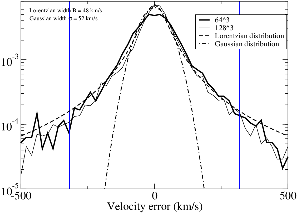
with $\beta=0.51$ for the studied simulation (corresponding to $\Omega_{m}=0.30$ ), $v_{\text{r}}$ the line-of-sight component of the simulated velocity of the considered, $\psi_{\text{r,rec}}$ the reconstructed radial displacement. The result is given in Fig. 5. We have tried to fit an histogram of the errors $\{e_{i}\}$ by both a Gaussian function of width $B$

f_{G}(e)\propto\exp\left(-\frac{e^{2}}{B^{2}}\right)

(9)

and a Lorentzian function

f_{L}(e)\propto\frac{1}{1+\frac{e^{2}}{B^{2}}}\;.

(10)

We obtained approximately the same width $B$ for the two fits (which is expected from the second order development of both functions), however it is striking that $f_{L}$ is a much better approximation than $f_{G}$ to the observed error distribution.

We equate the probability of getting an error $e$ on the true velocity $v_{\text{r}}$ for an object of the catalog to $f_{L}(e)$ . We also assume now that the distribution of velocities in the object sample is, for a sufficiently large volume, Gaussian with a width $\sigma_{v}$ :

P(v_{\text{r}}|\sigma_{v})\propto\exp\left(-\frac{v_{\text{r}}^{2}}{2\sigma_{v}^{2}}\right)\;.

(11)

Now we can build the joint probability of getting $v_{\text{r}}$ , $\psi_{\text{r,rec}}$ and $\beta$ :

P(v_{\text{r}},\psi_{\text{r,rec}},\beta|B,\sigma_{v})\\ \propto P(e(v_{\text{r}},\psi_{\text{r,rec}})|B,\sigma_{v})P(v_{\text{r}}|B,\sigma_{v})P(\psi_{\text{r,rec}}|B,\sigma_{v})\\ \propto P(\psi_{\text{r,rec}}|B,\sigma_{v})\frac{\exp\left(-\frac{v_{\text{r}}^{2}}{2\sigma_{v}^{2}}\right)}{1+\left(\frac{v_{\text{r}}-\beta\psi_{\text{r,rec}}}{B}\right)^{2}}\;,

(12)

where the constant of proportionality eventually depends on $B$ , $\sigma_{v}$ and $\beta$ . Using the theorem of Bayes, it is now possible to compute the conditional probability that the true velocity of some object is $v_{\text{r}}$ given that the reconstructed displacement is $\psi_{\text{r,rec}}$ :

P(v_{\text{r}}|\psi_{\text{r,rec}},\beta,B,\sigma_{v})\\ =\frac{\mathrm{e}^{-\frac{v_{r}^{2}}{2\sigma^{2}_{v}}}\left(1+\left(\frac{\beta_{*}\psi_{r}-\alpha_{*}v_{r}+\gamma_{*}}{B_{v}}\right)^{2}\right)^{-1}}{\int_{v=-\infty}^{+\infty}\mathrm{e}^{-\frac{v^{2}}{2\sigma^{2}_{v}}}\left(1+\left(\frac{\beta_{*}\psi_{r}-\alpha_{*}v+\gamma_{*}}{B_{v}}\right)^{2}\right)^{-1}\;\text{d}v}\;.

(13)

To obtain the total likelihood $\mathfrak{L}(\beta)$ to observe true velocities $\{v_{i,\text{r}}\}$ given that the reconstructed displacements are $\{\psi_{i,\text{r,rec}}\}$ , one may assume the statistical independence of the $(v_{i,\text{r}},\psi_{i,\text{r,rec}})$ duets. With this assumption, $\mathfrak{L}$ is simply

\mathfrak{L}(\beta)=\prod_{i}P(v_{i,\text{r}}|\psi_{i,\text{r,rec},\beta,B,\sigma_{v}})

(14)

Using that approach we have made measurements in finite volume mock catalogs. For example, with a PaddedDom reconstruction, one measure $\Omega_{\text{m}}=0.34$ with this approach (for an effective $\Omega_{\text{m}}=0.35$ in this catalog), whereas a naive measurement would yield $\Omega_{\text{m}}\leq 0.26$ .

VII Conclusion

We presented a method to predict velocities of galaxies from their current position. To solve this problem, we implemented a fast algorithm invented by Dimitri Bertsekas [3] and applied the method to a pure dark matter simulation. It happens that the reconstructed velocities are impressively accurate on large-scales (§ IV). However, the solution is only approximate in regions where multi-streaming occurs.

We proposed two methods for partially correcting boundary effects (§ V) and showed how boundary effects affect the reconstructed velocity field. We preferred the PaddedDom reconstruction scheme as it seems to give overall better results. Empirically we found that a buffer zone of 20 $h^{-1}$ Mpc is needed before obtaining a reconstructed velocity field correlated with the one given by the simulation.

At last, we proposed a bayesian model (§ VI) to account for reconstruction errors while estimating the slope between the reconstructed displacements and the true velocities of objects in a galaxy catalogs.

We would like to continue this work by improving the padding schemes to have even less boundary effects and make full use of available data in astronomy. We are also working on an improved algorithm that is able to take into account in a better way the non-linearities that are introduced in the velocity field due to gravitational effects occuring along particle trajectories. This new algorithm will try to fully solve the Euler-Poisson problem.²² 2 G. Lavaux & G. Loeper, work in progress.

This work is partially supported by the ANR grant BLAN07-2_183172 (project OTARIE).

References

[1] P. J. E. Peebles, Tracing galaxy orbits back in time, ApJL 344 (1989) L53–L56.
[2] Y. Brenier, U. Frisch, M. Hénon, G. Loeper, S. Matarrese, R. Mohayaee, A. Sobolevskiĭ, Reconstruction of the early Universe as a convex optimization problem, MNRAS 346 (2003) 501–524.
[3] D. P. Bertsekas, A Distributed Algorithm for the Assignment Problem, MIT Press, Cambridge, MA, 1979.
[4] R. Mohayaee, H. Mathis, S. Colombi, J. Silk, Reconstruction of primordial density fields, MNRAS 365 (2006) 939–959.
[5] H. M. P. Couchman, P. A. Thomas, F. R. Pearce, Hydra: an Adaptive-Mesh Implementation of P 3M-SPH, ApJ 452 (1995) 797–+.
[6] G. Lavaux, R. Mohayaee, S. Colombi, R. B. Tully, F. Bernardeau, J. Silk, Observational biases in Lagrangian reconstructions of cosmic velocity fields, ArXiv e-prints 707.