Continuous-time quantum walks on one-dimension regular networks
Abstract
In this paper, we consider continuous-time quantum walks (CTQWs) on one-dimension ring lattice of nodes in which every node is connected to its nearest neighbors ( on either side). In the framework of Bloch function ansatz, we calculate the spacetime transition probabilities between two nodes of the lattice. We find that the transport of CTQWs between two different nodes is faster than that of the classical continuous-time random walk (CTRWs). The transport speed, which is defined by the ratio of the shortest path length and propagating time, increases with the connectivity parameter for both the CTQWs and CTRWs. For fixed parameter , the transport of CTRWs gets slow with the increase of the shortest distance while the transport (speed) of CTQWs turns out to be a constant value. In the long time limit, depending on the network size and connectivity parameter , the limiting probability distributions of CTQWs show various patterns. When the network size is an even number, the probability of being at the original node differs from that of being at the opposite node, which also depends on the precise value of parameter .
pacs
05.60.Gg, 03.67.-a, 05.40.-aI Introduction
Quantum walks have important applications in various fields of solid-state physics, polymer chemistry, biology, astronomy, mathematics and computer science [1, 2, 3, 4, 5, 6]. A quantum random walk (QRW) is a natural extension to the quantum world of the ubiquitous classical random walk. It was first introduced in [7] and extensively investigated recently in connection with possible applications to quantum algorithms [8]. The behavior of quantum walks differs from that of the classical random walks in several striking ways, due to the fact that quantum walks exhibit interference patterns whereas the classical random walks do not. For instance, the mixing times, hitting times and exit probabilities of quantum walks can differ significantly from analogously defined random walks [9, 10, 11]. In recent years, two types of quantum walks exist in the literature: the discrete-time quantum coined walks and continuous-time quantum walks [12, 13]. Although both the two types of quantum walks have efficient quantum algorithms with respect to their classical counterparts, quantum walks show some advantages in dealing with decoherence processes compared to the discrete-time quantum algorithms, which are very sensitive to environmental quantum noise [14].
Here, we focus on continuous-time quantum walks (CTQWs). Most of previous studies consider CTQWs on simple structures, such as, the line [15, 16], cycle [17, 18], hypercube [19], Cayley tree [20], dendrimers [21] and other regular networks with simple topology. Although CTQWs have received much attention and there has been some work about CTQWs on general graphs, many questions about CTQWs appear to be quite difficult to answer at the present time. For simple structures these quantum walks are analytical solvable and directly related to the well-known problems in solid state physics. Recently, Oliver Mülken et al have studied the spacetime structures of CTQWs on one-dimensional and two-dimensional lattices with periodic boundary conditions [22, 23]. The topology of the lattices they considered is oversimplified, i.e., each node is only connected to its two nearest neighbors. For regular graphs with symmetrical structure, the dynamics of the quantum transport is determined by the topology of the network. To this end, it is natural to consider quantum transport on general lattices with more connectivity.
In this paper, we study CTQWs on one-dimension ring lattice of nodes in which every node is connected to its nearest neighbors ( on either side). This generalized regular network has broad applications in various coupled dynamical systems, including biological oscillators [24], Josephson junction arrays [25], neural networks [26], synchronization [27], small-world networks [28] and many other self-organizing systems. We analyze quantum walks on such general network with periodic boundary conditions using the Bloch function approach [29], which is commonly used in solid state physics. We derive analytical expressions for the transition probabilities between two nodes of the networks, and compare them with the results of CTRWs.
The paper is structured as follows: In Sec. II we review the properties of CTQWs presented in Ref.[30] and give the exact solutions to the transition probabilities on the general ring network. Section III presents the time evolution of the probabilities. In Sec. IV, we consider the distributions of long time limiting probabilities. Conclusions and discussions are given in the last part, Sec. V.
II Continuous-time quantum walks
Keeping in line with previous results on quantum walks, we study continuous-time quantum walk on networks and compare the results with the classical counterparts.
II.1 Continuous-time quantum walks on general networks
We consider a walk on a general graph, which is a collection of connected nodes and simple links without weight and directions. The topology of such simple graphs can be described by the corresponding Laplace matrix . The nondiagonal elements equal to if nodes and are connected and otherwise. The diagonal elements equal the number of total links connected to node , i.e., equals to the degree of node . Classically, the evolution of continuous-time random walk is governed by the master equation [3]
| (1) |
Where is the conditional probability to find the CTRW at time at node when starting at node . Matrix is the transfer matrix of the walk, and relates to the Laplace matrix by . Here, for the sake of simplicity, we assume the transmission rate for all connections to be equal. Then the solution of the above equation is
| (2) |
Quantum mechanically, the dynamical evolution equation of continuous-time quantum walks is obtained by replacing the Hamiltonian of the system by the classical transfer matrix, [9, 10]. The states endowed with the nodes of the network form a complete, ortho-normalised basis set, which span the whole accessible Hilbert space, i.e., , . The time evolution of state is given by the Schrodinger Equation (SE)
| (3) |
Where the mass and is assumed in the above equation. Starting at time from the state , the evolution equation of the state is , where is the quantum mechanical time evolution operator. The transition amplitude from state at time to state at time is
| (4) |
Combining Eq. (3), we have
| (5) |
We note that the different normalization for CTRWs and CTQWs. For CTRWs, and quantum mechanically holds.
To get the exact solution of Eqs. (1) and (5), all the eigenvalues and eigenvectors of the transfer operator and Hamiltonian are required. We use to represent the th eigenvalue of and denote the orthonormalized eigenstate of Hamiltonian by , such that . The classical transition probability between two nodes is given by
| (6) |
And the quantum mechanical transition probability between and is
| (7) |
For finite networks, do not decay ad infinitum but at some time fluctuates about a constant value. This value is determined by the long time average of
| (8) |
II.2 Continuous-time quantum walks on 1D ring lattice and Bloch ansatz solutions
In the subsequent calculation, we restrict our attention on CTQWs on the general one-dimension ring lattices with periodic boundary conditions. The network organizes in a very regular manner, i.e., each node of the lattice is connected to its nearest neighbors ( on either side), thus the Laplace matrix takes the following form,
| (9) |
The Hamiltonian of the system is given by . For simplicity of analytical treatment, we set in further calculations. The Hamiltonian acting on the state can be written as
| (10) |
The above Equation is the discrete version of the Hamiltonian for a free particle moving on the lattice. Using the Bloch function approach [29] for the periodic system in solid state physics, the time independent SE reads
| (11) |
The Bloch states can be expanded as a linear combination of the states localized at node ,
| (12) |
Substituting Eqs. (10) and (12) into Eq. (11), we obtain the eigenvalues (or energy) of the system,
| (13) |
The periodic boundary condition for the network requires that the projection of on the state equals to that on the state , thus with integer and . Replacing by the Bloch states in Eqs. (6), (7), we can get the classical and quantum transition probability
| (14) |
| (15) |
For infinite networks, i.e., , Eqs. (14) and (15) translates to
| (16) |
| (17) |
Particularly, when , the network corresponds to a cycle graph where each node has exact two nearest neighbors. The limiting transition probability can be rewritten as and , where is the Bessel function of the first kind [31]. This is consistent with the result in Ref. [23]. The difference between finite and infinite network is that, for infinite networks the interference of quantum transport is weak compared to finite networks. For larger value of , the above analytical expression could not be further simplified. We can calculate the transition probabilities straightly using the integrations for the infinite networks. We will show that there is some difference of the transition probabilities between finite and infinite networks at long time scale.
Finally, the long time averaged probability between two nodes yields
| (18) |
Interestingly, the long time averaged probability is related to the spectral of the networks, in contrast to the classical transport where there is a uniform probability () to find the walker at every node. The time limiting probabilities depend on the degeneracies of the eigenvalues, which result in odd, unexpected patterns of limiting probability distributions.
III Time evolution of the probabilities
In this section, we analyze the time dependent probabilities of the theoretical calculations. The numerical determination of the eigenvalues, eigenvectors and integration is done using the software Mathematica. Specifically, we perform our calculations on infinite and finite () networks with different connectivity .
III.1 Return probabilities
The probability to be still or again at the initial node is a good measure to quantify the efficiency of the transport [32]. Classically, according to Eq. (14), the probability of being at the original node is
| (19) |
Which only depends on the eigenvalues. The quantum-mechanical probability of finding the walker at the initial node is given by Eq. (15),
| (20) |
Which also dependents on the eigenvalues of the system. The return probability is independent on the position of the initial excitation nodes because of the symmetry of network topology. Analogously, employing the relation of , we can calculate the return probabilities on infinite networks according to Eqs (16) and (17).
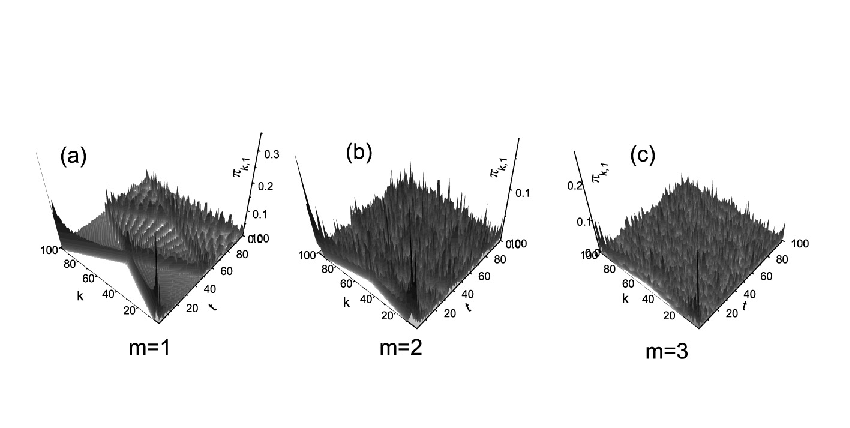
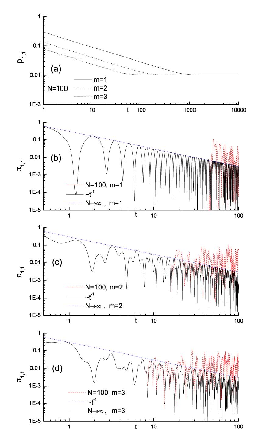
Fig.1 shows the return probabilities for CTRWs and CTQWs. Consider a CTRW on a network of size and assume the initial excitation starts at node . Fig.1 (a) depicts the temporal behavior of return probability with different values of . There is a power law decay () at the beginning of the transport, but after some time reaches a constant value. This time is determined by the time when reaches the equipartitioned probability . The time becomes small when the parameter increases, this indicates that it takes less time for the return probability to reach the equipartitioned probability on networks with high connectivity. Fig.1 (b), (c) and (d) shows the quantum mechanical return probabilities for , , and , respectively. The dashed curves show the results on network of and the black solid curves show the results on infinite network according to Eq. (17). The dashed lines indicate the scaling behavior . We note that the return probabilities of finite and infinite networks agree with each other in small time scales. At later times waves propagating on the finite networks start to interferer, this leads to the probabilities differ and the deviation happens at earlier times on highly connected networks (with larger value of ). Furthermore, the return probabilities oscillate frequently on highly connected networks and there are more peaks compared to networks with small value of . Such a behavior may be attributed to the fact that the interferences on networks with high connectivity are stronger than on those with small connectivity.
III.2 Transition probabilities and transport velocity
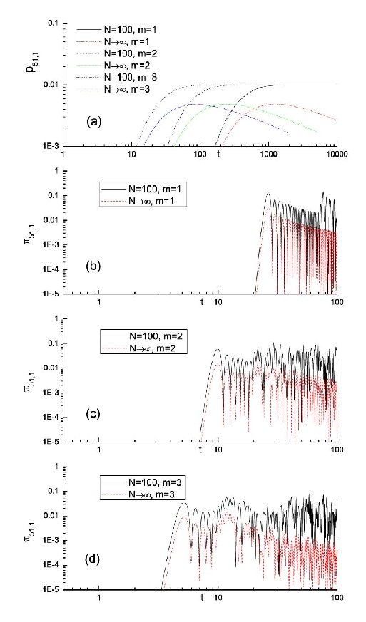
The transition probabilities between two different nodes provide us more information about the transport process over the whole network. For a finite network of , we consider the probability of finding the walker at the opposite node. Fig. 2 shows the transition probabilities for CTRWs and CTQWs. In Figure 2, (a) shows the classical transition probabilities on infinite and finite networks of size with different values of . As we can see, the transition probabilities on finite networks with more connectivity approach to the equipartitioned probability quicker than those on network with less connectivity. For infinite network, the transition probabilities increase with time in the first period, and then reach the maxima and decrease in the large scale time. Quantum mechanically, the transition probabilities for , , and are shown in Fig. 2 (b), (c) and (d). The dashed curves are the results for network of , solid curves are the corresponding results for infinite networks. The transition probabilities on infinite networks are smaller than those on finite networks at the same time. Interestingly, for the same connectivity parameter , the character time when the first maximum of the probabilities occur on finite networks equals to that on infinite networks, i.e., the character time is independent on the size of the networks.
The probabilities to go from a starting node to all other nodes in time on a network of size with different values of are plotted in Fig. 3. The starting excitation is located at node , and we can see the time propagating to the opposite node becomes small on networks with large value of . In addition, the structure is quite regular when . As increases, the pattern becomes irregular.
In order to compare the transport speed on different networks, we define the character time as the time when the first maximum of the probabilities occur on infinite networks. Such definition is held both for the classical and quantum transport. For the classical transport, there is only one maximal value and the character time corresponds to the time when the equipartitioned probability is reached on finite networks. Now it is natural to ask the question : Does the transport take equal time between two nodes of the same shortest path length? To address this question, we calculate the transition probabilities between two nodes having the same value of shortest path length on infinite networks. Fig. 4 (a) shows the classical transition probabilities , and for , and . The shortest path lengths of the two nodes for the three infinite networks equal to , but the character time is small for highly connected networks. This indicates that the transport is quick on networks with high connectivity for CTRWs. For CTQWs, the same conclusion is also true, as confirmed by the corresponding plot in Fig. 4 (b). The character time for the quantum transport is much smaller than that of the classical one, this supports the fact that the quantum walks have efficient quantum algorithms with respect to their classical counterparts [33].
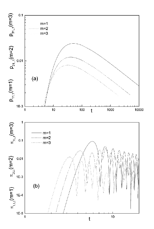
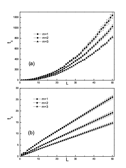
Fig. 5 shows the character time versus the shortest path length on networks with different values of . For classical transport (Fig. 5 (a)), grows faster than the shortest path length . It is found that the relationship between the character time and the shortest path length can be well described by quadratic equation: , where the parameter can be obtained by fitting the data. Defining the transport speed as the ratio of and , we find that the classical transport speed gets slow for large while the quantum transport speed turns out to be a constant values. We note that the transport speed is large on highly connected networks even the two nodes are located at the same distance . By fitting the linear relation between and , the quantum transport velocities are estimated to be about , and for , and respectively. The different behavior of the transport velocities between CTRQs and CTQWs is a striking characteristic that distinguishes the classical and quantum transport processes.
IV Long time limiting probabilities
Now, we consider the long time averaged probabilities. Classically, the long time liming probabilities equal to the equipartitioned probability [23]. Quantum mechanically, the limiting probabilities are determined by Eq. (18) but the situation is more complex for different network parameters. For , the spectral (or energy) of the system is , where , . If the network size is an even number, there are two nondegenerate eigenvalues, and , and other eigenvalues have degeneracy 2. The limiting probabilities can be written as
| (21) |
If the network size is an odd number, there are one nondegenerate eigenvalues , and the other eigenvalues have degeneracy . The limiting probabilities can be summarized as
| (22) |
Which confirms the results in Ref. [30].
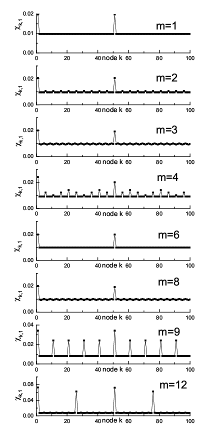
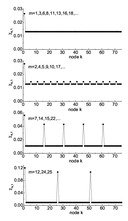
For other values of , the limiting probability distributions can also be determined according to the degeneracy distribution of the eigenvalues, but such process is complicated for large values of . Here, we report the limiting probabilities numerically obtained using the Eq. (18). In Fig. 6, we display the limiting probabilities on the network of size with the starting node . As we can see, the probabilities for and are the same as and . After a careful examination, we find that and have the same degeneracy distribution of eigenvalues, and and have the same degenerate eigenvalue distribution. Particularly, for all the values of , there is a large probability to be still or again at the initial node and at the opposite node . For some values of , the probabilities at the two positions are extremely high, for instance, when , the return probabilities exceed . For odd number of network size, there is a higher probability to find the walker at the initial node than that at other nodes. For networks of size and , the limiting probability distribution shows the same pattern described as Eq.(22). One may conjecture that the pattern of does not change when increasing parameter on odd-numbered networks, but this is not true for some values of network size . For instance, on networks of size with some particular values of , the limiting probability distribution differs from the pattern of Eq.(22) (See Fig. 7). It is interesting to note that the patterns of are the same for some values of , this feature can be explained by the identical degeneracy distribution of the eigenvalues for different values of .
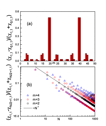
As we have shown, if the network size is an even number, there are high probabilities to find the walker at the initial node and the opposite node. For some values of , we find that the probability of being at the initial node equals to the probability of being at the opposite node. However, for some other values of , this is not true. In Ref. [30], the authors find asymmetry of the probabilities for the starting node and its mirror node, their definition of mirror node is based on geometry symmetry of the network. In this paper, we define the mirror node of a given node to be its opposite node, i.e., . We find asymmetry of the probabilities of being at the initial node and at the opposite node (mirror node) for some particular network parameters and . Such asymmetry is small and not easy to be observed in Fig. 6. For a network of size and assuming the initial exciton starts at node , we find that asymmetries occur at …. The asymmetrical limiting probabilities are particularly characterized by the difference between and , thus we use the quantity to detect the asymmetry of the probabilities. In Fig. 8 (a), we present as a function of parameter . There are distinct values of having asymmetrical probabilities, which is indicated by the nonzero value of .
To reveal a general dependence of the asymmetry on the network parameters, we plot the quantity as a function of the network size for different values of , which are shown in Fig. 8 (b). For , the probabilities are symmetrical for all the network size , thus we only show the asymmetry for , , and . We find that the points break into several clusters, whereas some clusters decreases with the network size as a power law: .
Except for the asymmetrical probabilities between the initial node and the opposite node (mirror node), we also find asymmetrical probabilities between other nodes and their mirror nodes. In our calculations, we find that such asymmetries can be different from the asymmetry of the probability of being at the initial node and being at its opposite node. For instance, considering a CTQW on a network of size and assuming the initial excitation starts at node , there are asymmetries between and ( is an even number) for some values of . The discrete values of for different asymmetries can differ from each other, depending on the precise value of and . This situation is even more complex and requires a further study.
V Conclusions and Discussions
In summary, we have studied continuous-time quantum walks on one-dimension ring lattice of nodes in which each node is connected to its nearest neighbors ( on either side). Using the Bloch function approach, we calculate transition probabilities between two nodes of the lattice, and compare the results with the classical counterpart. It is found that the transport of CTQW is faster than that of the classical continuous-time random walk. We define the transport velocity as the ratio of the shortest path length and spreading time between two nodes. For network of a given parameter , the transport of CTRWs gets slow with the increase of the shortest distance while the transport of CTQWs spreads the network constantly. In the long time limit, depending on the network parameters and , the limiting probability distributions of CTQWs show various patterns. When the network size is an even number, the probability of being at the original node differs from that of being at the opposite node, which also depends on the precise value of parameter . Asymmetrical probabilities between other nodes and their mirror nodes also exist for some particular network parameters.
The asymmetry of the limiting probabilities of being at a node and being at its mirror node is a novel phenomenon, which does not exist in the cycle graph with . However, we are unable to predict which particular parameters of and are related to such asymmetry. Furthermore, in our calculations, we find a large value of the limiting return probability for some special network topology, for instance, on a complete graph in which each pair of nodes is connected, the long time averaged return probabilities equal to while the other transition probabilities are (). This is a striking feature of CTQWs which differs from the classical counterpart.
Acknowledgements.
The authors would like to thank Zhu Kai for converting the mathematical package used in the calculations. This work is supported by the Cai Xu Foundation for Research and Creation (CFRC), National Natural Science Foundation of China under projects 10575042, 10775058 and MOE of China under contract number IRT0624 (CCNU).References
- [1] T. Odagaki and M. Lax, Phys. Rev. B 24, 5284 (1981).
- [2] T. Odagaki and M. Lax, Phys. Rev. B 26, 6480 (1982).
- [3] G. H. Weiss, Aspect and Applications of the Random Walk (North-Holland, Amsterdam, 1994).
- [4] J. Kempe, Contemp. Phys. 44, 307 (2002).
- [5] D. Supriyo, Quantum Transport: Atom to Transistor (Cambridge University Press, London, 2005).
- [6] A. Ambainis, Quantum search algorithms (New York, USA , 2004).
- [7] Y. Aharonov, L. Davidovich, and N. Zagury, Phys. Rev. A 48, 1687 (1993).
- [8] N. Shenvi, J. Kempe, and K. Brigitta Whaley, Phys. Rev. A 67, 052307 (2003).
- [9] E. Farhi and S. Gutmann, Phys. Rev. A 58, 915 (1998).
- [10] A. M. Childs, E. Farhi, and S. Gutmann, Quant. Inf. Proc. 1, 35 (2002).
- [11] H. Gerhardt and J. Watrous, quant-ph/0305182.
- [12] N. Konno, Phys. Rev. E 72, 026113 (2005).
- [13] A. Ambainis, J. Kempe and A. Rivosh,Coins make quantum walks faster (Philadelphia, USA, 2005).
- [14] D. Shapira, O. Biham, A. J. Bracken, and M. Hackett, Phys. Rev. A 68, 062315 (2003)
- [15] N. Ashwin and V. Ashvin, quant-ph/0010117.
- [16] G. Abal, R. Siri, A. Romanelli, et al., Phys. Rev. A 73, 042302 (2006)
- [17] D. Solenov and L. Fedichkin, Phys. Rev. A 73, 012313 (2003)
- [18] F. Sorrentino, M. di Bernardo, G. H. Cuéllar, and S. Boccaletti, Physica D 224, 123 (2006).
- [19] H. Krovi and T. A. Brun, Phys. Rev. A 73, 032341 (2006).
- [20] O. Mülken and A. Blumen, Phys. Rev. E 71, 016101 (2005).
- [21] O. Mülken, V. Bierbaum and A. Blumen, J. Chem. Phys 124, 124905 (2006).
- [22] O. Mülken and A. Blumen, Phys. Rev. E 71, 036128 (2005).
- [23] A. Volta, O. Mülken and A. Blumen, J. Phys. A 39, 14997 (2006).
- [24] S. H. Strogatz, and I. Stewart, Sci. Am. 269, 102 (1993).
- [25] K. Wiesenfeld, Physica B 222, 315 (1996).
- [26] L. F. Abbott and C. V. Vreeswijk, Phys. Rev. E 48, 1483 (1993).
- [27] I.V. Belykh, V.N. Belykh and M. Hasler, Physica D 195, 159 (2004).
- [28] D. J. Watts and S. H. Strogatz, Nature 393, 440 (1998).
- [29] C. Kittel, Introduction to solid state physics (Wiley, New York, 1986).
- [30] O. Mülken, A. Volta and A. Blumen, Phys. Rev. A 72, 042334 (2005)
- [31] G. E. Andrews, R. Askey and R. Roy, Special functions (Tsinghua Univ, China, 2004).
- [32] O. Mülken and A. Blumen, Phys. Rev. E 73, 066117 (2006).
- [33] P. C. Richter, Phys. Rev. A 76, 042306 (2007).