Impact of Electric Current Fluctuations
Arising from Power Supplies and Space Charge
on Charged-Particle Beams:
A Measurement-Based Stochastic Noise Model of Fermilab’s Booster Synchrotron
Abstract
Electric current fluctuations are one type of unavoidable machine imperfections and induce magnetic-field perturbation as a source of instabilities in accelerators. This paper presents the measurement-based modeling methodology of fluctuating electric current arising from the power system of Fermilab’s Booster synchrotron to discuss the ramifications of the presence of ripple current and space-charge defocusing effects. We also present the method of generating stochastic noise and the measurement and analysis methods of ripple current and offending electromagnetic interferences residing in the Booster power system. This stochastic noise model, accompanied by a suite of beam diagnostic calculations, manifests that the fluctuating power-supply current, when coupled to space charge and impinging upon a beam, can substantially enhance beam degradation phenomena—such as emittance growth and halo formation—during the Booster injection period. With idealized and uniform charge-density distribution, the fractional growth of rms emittances due to ripple current under space charge turn out to be about in both transverse planes over the injection period of 2.2 ms prior to beam acceleration.
Keywords:
accelerator physics; accelerator modeling; beam injection; cyclic accelerators; stochastic noise; space charge; power supplypacs
05.40.-a, 07.05.Tp, 29.20.D-, 43.50.Yw, 43.60.Cg, 47.75.-i, 77.22.Jp, 84.30.JcI INTRODUCTION AND MOTIVATION
As is common in other natural systems, subtle fluctuations are ubiquitous and inevitable in particle accelerator systems. An ensemble of charged particles is defined as a system, and all the beamline components (magnets, power supplies, RF cavities, beam position monitors, etc.) for accelerating, guiding, and diagnosing particle beams as environment, or surroundings. The system of a charged-particle beam perceives the environment of beamline components as a source of noise as illustrated by FIG. 1.

External noise is intrinsic to particle accelerators of all types due to unavoidable machine imperfections; e.g., ripple current from power supplies, ground vibration motion, etc. After being motivated by earlier findings from an idealized and simplified theoretical model [1], we speculated that the adverse influence of power-supply current fluctuations possibly account for beam loss phenomena observed during the injection process of the Booster. Hence, an independent and novel approach has been made to build a realistic stochastic noise model, based upon a series of power-supply noise11 1 In the present context, we will use the terms (power-supply) noise and current fluctuations and ripple current interchangeably. measurements, to investigate and explore the impact of current fluctuations on charged-particle beams of the Booster at injection energy of 400 MeV.
II MODELING METHODOLOGY
For investigations of the impact of power-supply current fluctuations on charged-particle beams in an accelerator lattice structure, we began with building a preliminary noise model. As a first step, we designed and added a new physics module for generating stochastic noise to the existing ORBIT-FNAL package [2]. The new noise module is capable of generating a wide spectrum of stochastic noise employing the Ornstein-Uhlenebck stochastic process [3] that is governed by a Langevin-like stochastic differential equation [4].
Prior to detailed experimental measurements, we corroborated with the preliminary noise model using a linear lattice that non-white, or colored noise could possibly enhance beam degradation process of our interest. These preliminary findings are consistent with earlier findings from the theoretical model of collective space-charge modes coupled with dynamic noise [1]. As a next step, in addition to adding the new noise module to the ORBIT-FNAL, the existing TeaPot module was upgraded to establish Fermilab’s Booster ring using a TEAPOT-style [5] Booster lattice, and the Diagnostic module with new parallelized beam diagnostic calculations: actions, halo amplitudes, etc.


As confirmed with the preliminary model, we proceeded to devise methods for direct measurements of common-mode and differential-mode voltages, and ripples in the electric current. Repeated measurements and Fourier analysis confirm that a substantial amount of noise, which can be transmitted to the magnet system, is indeed present in the power system. Moreover, we performed equivalent-circuit simulations to investigate any offending resonances that can float around the magnet system. Based upon the measurement data and the results of Fourier analysis, stochastic parameterization of Booster ripple current is performed by means of matching power spectral densities between measured ripple currents and modeled Ornstein-Uhlenbeck (O-U) noise [3]. While translating modeled O-U noise to induced magnetic-field fluctuations, we tracked macroparticles in the presence of 3-D space-charge effects.
The following FIG. 2 and FIG. 3 illustrate the multi-stage approach to the stochastic noise modeling. For the purpose of the stochastic parameterization of ripple current, mapping from an experimental signature space to a stochastic parameter space was done; the preliminary model was faithfully tuned up with the power-supply noise measurements. As a consequence, we managed to match FFT power spectral densities between physical noise and modeled O-U noise.
III CLASSIFICATIONS OF NOISE
In general, noise can be categorized into two types: external noise and internal noise. In our stochastic noise model, ripple current arising from Gradient Magnet Power Supply (GMPS) units of the Booster are regarded to be fluctuating external influences acting on the Booster beam (see FIG. 1).
III.1 External Noise
External noise is originated from a source outside of the system; that is, beamline components. Since the effects of external noise can be described by a stochastic differential equation (SDE)22 2 A stochastic differential equation is a differential equation (DE) in which the coefficients are random functions of the independent variable, which is usually time., we chose Langevin Equation (LE) as SDE for indeterministic current fluctuations arising from each GMPS unit33 3 The Booster power supply will be frequently referred to as GMPS.. It should be noticed that power-supply ripple currents are considered indeterministic, or random, or aperiodic, in the sense that it never exactly repeats itself.
III.2 Electromagnetic Interferences
Electromagnetic-Interference (EMI) noise [7, 8] results from rapid changes in voltage and current in a power supply. Transmissions of EMI noise are characterized as either radiative, or conductive. Conductive EMI noise, such as differential-mode (DM) and common-mode (CM) noise, is usually several orders of magnitude higher than the radiative EMI, and can be more harmful to the system. Given impedance () as a function of frequency , fluctuations in common-mode voltage () create common-mode current (), in addition to the inherent ripple current arising from sudden potential changes in the power-supply system. The EMI problem is thereby worsened and could result in larger current fluctuations, or common-mode current, or severe system damage.
IV STOCHASTIC PROCESS
Of several different stochastic processes44 4 In this paper, we use terms stochastic process, stochastic function, random process, random function and process interchangeably., such as Poisson process, Wiener process, etc., we chose the Ornstein-Uhlenbeck process to represent electrical current fluctuations as classified in the preceding subsection.
IV.1 Langevin Equation
In 1908, after the formulation of the Brownian movement by Einstein and Smoluchowski [9, 10], P. Langevin introduced the concept of the equation of motion of a stochastic variable (i.e., the position coordinate of a Brownian particle) [11]. Langevin Equation (LE) is considered to be the first example of a Stochastic Differential Equation (SDE)55 5 A stochastic differential equation is a differential equation with a stochastic (random) term. Therefore, its solution is also a random function.. Langevin wrote the equation of motion for a Brownian particle according to Newton’s second law under the assumption that a Brownian particle is subject to two forces: damping force () and fluctuating force ()
| (1) |
| (2) |
Here, , , , and represent the total force, particle mass, displacement, and the friction coefficient, respectively. The first term (66 6 The notations, and , denote and , respectively.) on the right-hand side of Eqn. (2) represents the viscous drag as a function of time, or dynamic friction. The second term represents fluctuations which could be from white noise77 7 White noise is noise with a flat frequency spectrum. or non-white noise. The form of Eqn. (2) can be transformed to Eqn. (3) of first order. For modeling physical noise of the Booster power system, we employed non-white noise, or off-white noise in our investigations.
| (3) |
where is a stochastic driving force, and represents /. The following assumptions are made about the fluctuation part :
- (1)
is a function of time only, and independent of .
- (2)
zero-mean distribution;
(4) - (3)
The variation rate of is much faster than the velocity of a Brownian particle, . Hence, the autocorrelation function is of Dirac- function; i.e.,
| (5) |
The expressions above define the statistical properties of . There is a great advantage in using LE instead of using Fokker-Planck Equation (FPE) of mathematical complex. The Langevin’s method is much easier to understand than the FPE since it is based upon the time evolution of a stochastic variable, whereas the FPE applies to the time evolution of the probability distribution. As such, LE allows us to dispense with the calculation of the diffusion coefficient, thus reducing associated mathematical complications. As a consequence, we built an effective but far more simplified model of stochastic noise.
IV.2 Ornstein-Uhlenbeck Process
As in Eqn. (3), LE for Brownian motion is given as,
| (6) |
As explained in the preceding subsection,
LE is associated with -correlated
Gaussian stochastic forces
of statistical properties.
This stochastic process is referred to as an O-U process.
Note that the noise strength
does not dependent upon the variables .
Since the O-U stochastic process
is inherently to represent the velocity of a Brownian particle,
it is the appropriate choice of stochastic process
for modeling electric noise, or current fluctuations [3];
i.e., a time-derivative of electric charge ().
Both position () and velocity () describe
Langevin’s Brownian motion.
However, by utilizing the O-U process of
the velocity of a Brownian particle,
LE can be reduced to a -order
linear stochastic differential equation
that is derived from Newton’s law.
As a result,
LE as a -order SDE
is straightforward to find solutions.
The O-U process is associated with an exponentially-decreasing
autocorrelation function [12]
and a finite autocorrelation time [3]88
8
The autocorrelation function
determines the property of a stochastic process of interest..
| (7) | ||||
in which , , and are a stochastic function, an autocorrelation frequency, and a constant noise strength, respectively. O-U processes are associated with the following probability density function:
| (8) |
According to the Doob’s theorem [13], the O-U process is the only stochastic process with all of the following properties: (1) stationary process, (2) Gaussian process, (3) Markovian process. In particular, if a process is invariant to translations in time (e.g. a shift in time ()) then the process is called a stationary process [14, 4]. For a stationary process, we can make the following simplifications:
| (9) |
where is the stochastic function and is the statistical average. The form of Eqn. (9) implies the followings:
- (1)
Since the underlying mechanisms causing the fluctuations do not change with time, the stochastic properties of a stationary process are conserved.
- (2)
The important parameter in the O-U process is relative time and not the absolute time.
(10) Therefore, the autocorrelation function for a stationary process is a function of only.
- (3)
The ensemble average and the time average are the same, which leads to the ergodic property.
IV.3 Markov Process
Markov processes involve the use of conditional probability.
| (11) |
The Markov process is therefore defined as follows [4]:
| (12) |
The form of Eqn. (12) implies that all the for can be derived, when only is known. In other words,
Only the present condition determines the future condition.
In order to avoid unnecessary mathematical complexity in building a stochastic noise model, we exploited the Markovian property. This is another reason why, of all the stochastic processes, the O-U process is the most convenient choice for modeling the Booster ripple current.
V NON-WHITE NOISE GENERATION
V.1 Stochastic Properties
Langevin Equation governs an O-U process. Hence, if we use an O-U process to model GMPS current fluctuations, we need to solve LE. By solving the convenient -order linear LE, we were able to extract more statistical properties of the O-U process besides Eqns. (4), (5), and (8).
Let us first consider a -order SDE of the form of LE.
| (13) |
Here is non-white Gaussian noise with the autocorrelation function :
| (14) |
Non-white noise is governed by LE with a white-noise driving force of :
| (15) |
The autocorrelation function is -correlated with a strength :
| (16) |
Ornstein and Uhlenbeck [3], Doob [13], and van Kampen [4] use the integration method to find the statistical properties of non-white noise, or colored noise from LE. We, on the other hand, solve LE as a 1st-order DE. The general solution of a 1st-order inhomogeneous DE is a linear superposition of a homogeneous solution () and a particular solution (). Hence,
| (17) |
From Eqn. (17), the stochastic process at the next time step can be obtained.
| (18) |
Let be the second term of Eqn. (18).
| (19) |
By transforming the variables of integration, we can obtain
| (20) |
By squaring Eqn. (20), we arrive at
| (21) |
The statistical properties of a random variable can be investigated by the calculations of various moments. We calculate the first and the second central moments99 9 When a mean value of a variable is included in the moment calculation, it is referred to as central moment. by averaging Eqns. (20) and (21) over an ensemble of particles. The first two moments determine the complete statistical properties of the O-U noise because it is a zero-mean Gaussian process. For zero-mean Gaussian, the moment vanishes.
| (22) |
Accordingly, keeping in mind that the O-U process is a stationary process, the moments boil down to
| (23) |
The second moments of can be expanded in a closed form as in Eqn. (24).
| (24) | ||||
with being . What determines the is , which is time step in units of autocorrelation time , not autocorrelation time, or time step by itself. This module is designed to generate O-U stochastic noise that is to be applied to macroparticles in the form of magnetic-field perturbation: autocorrelation time (), time step (), and noise strength ().
V.2 Box-Muller-Like Transformation
The Box-Muller (BM) transformation [15, 16] is intrinsically for generating independent Gaussian white noise —which is a limiting case of physical noise— from independent uniform random deviates. In order to generate exponentially-driven Gaussian stochastic noise, an exponential factor, is first multiplied by the stochastic noise at present time . Then, a root-mean-square (rms) value of is added to compute the noise at the next time step .
| (25) | ||||
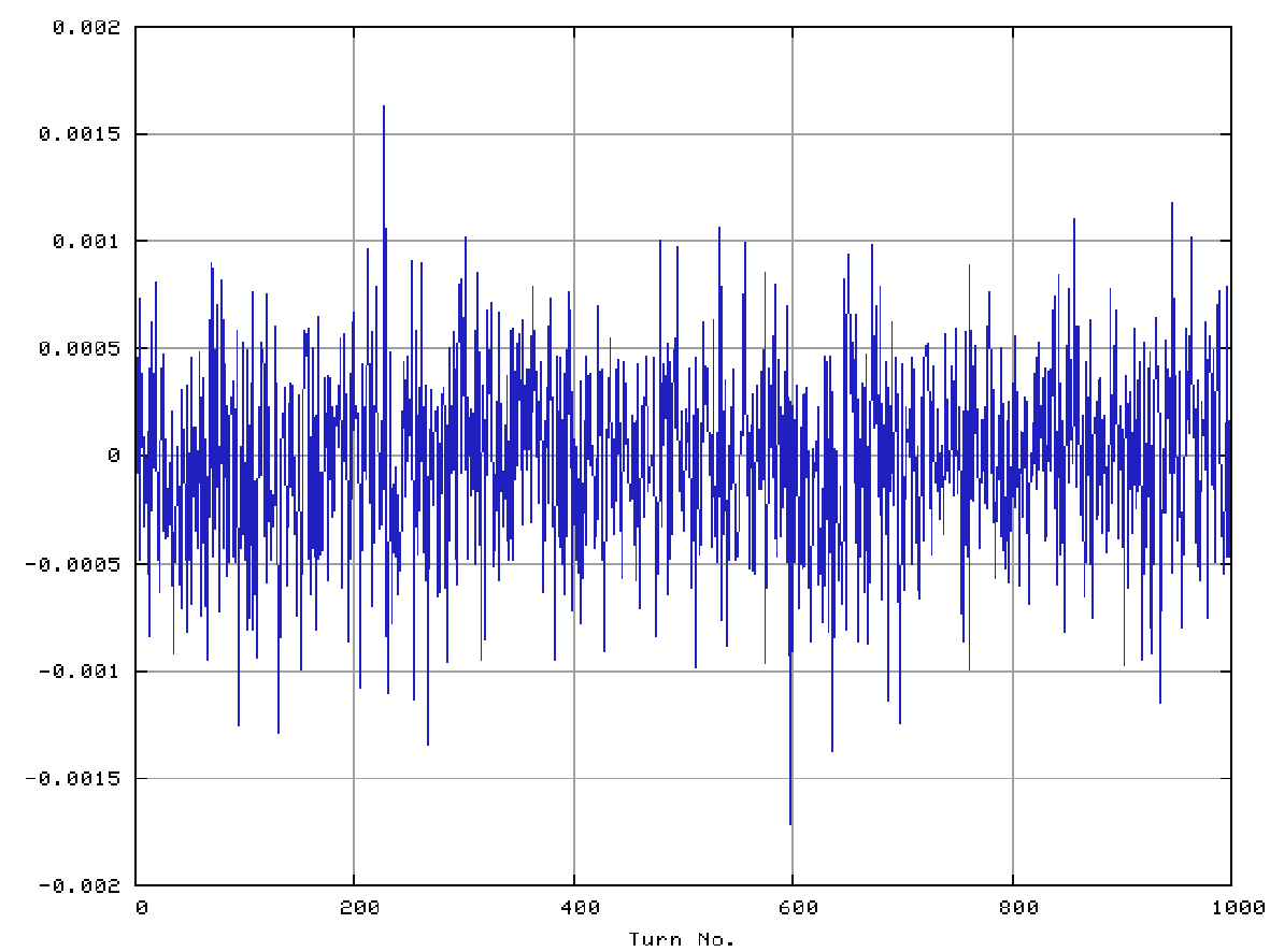
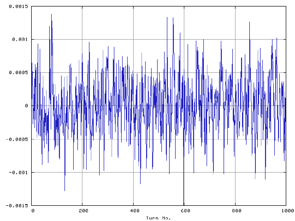
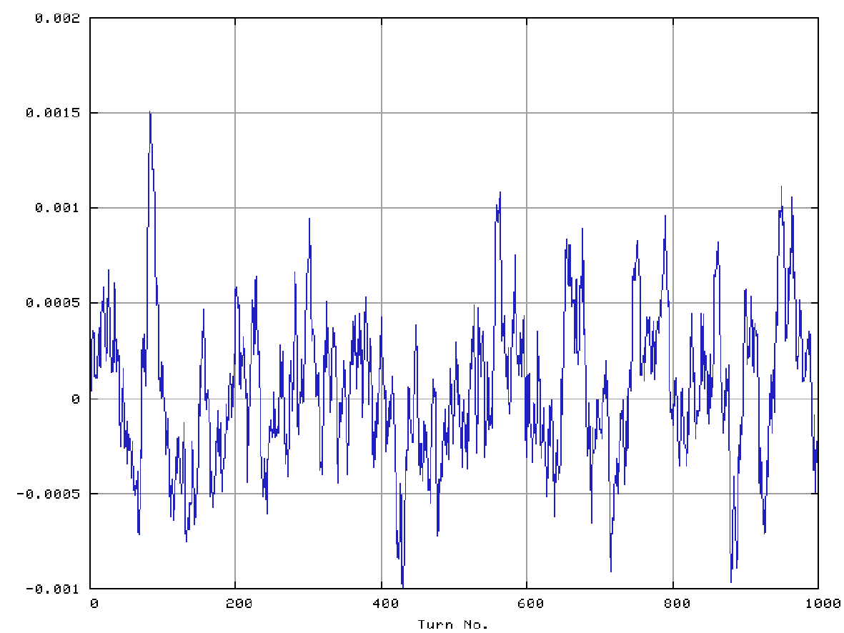
where denotes random deviates from a rectangular distribution (or white noise). What Eqn. (25) implies is that to generate , one needs to know only. This takes advantage of the powerful Markov property of the O-U process in numerical calculations. Upon providing with stochastic parameters, the variant of the BM transformation is capable of generating a wide spectrum of stochastic noise: colored noise, non-white noise, off-white noise, etc. Sample paths of different noises that are generated from the new noise module are plotted in FIG. 4: the autocorrelation time () ranges from 10-3 ( denotes one revolution period.) to . The time step is fixed at one revolution period at the Booster injection energy. FIG. 4 demonstrates that the autocorrelation time governs the pattern of sample path. It is therefore evident that the pattern of all sample paths are aperiodic. More details of the non-white noise algorithm can be found elsewhere [17].
V.3 Application of Noise to Macroparticles
Since current fluctuations are directly proportional to magnetic-field fluctuations, in the noise model the ripple-current measurements are translated into magnetic-field fluctuations as in Eqn. (26).
| (26) |
where denotes magnet index for differentiating between each individual main magnets. In order to distinguish field fluctuations at each type of magnet (, or ), is factored out, and the amount of field variation () is normalized by as a perturbation term.



VI GRADIENT-MAGNET POWER-SUPPLY (GMPS) SYSTEM
The Gradient Magnet Power Supply (GMPS) System for the Booster synchrotron powers a total of 96 main gradient magnets1010 10 The gradient magnet is referred to as the combined-function magnet of the Booster.. A resonance system is selected in order to reduce the size and the cost of the power-supply system. The Booster magnet system consists of 48 LC-resonant magnet cells. A focusing magnet (F), a defocusing magnet (D), a choke, and a capacitor bank constitute an individual magnet cell. In turn, 48 focusing and 48 defocusing magnets are connected in series by common buses. Since the gradient magnets are powered by four independent power supplies (GMPS) that are symmetrically inserted in the LC-resonant system, the GMPS voltages to ground ( and ) can be kept as low as possible. Each GMPS drives current at the fundamental frequency of 15 Hz through a string of 12 magnet cells. The GMPS system includes dual three-phase Silicon Controlled Rectifier (SCR) bridges connected in series, and fed by a 12-phase 13.8-kV bus with shunt (or stray) capacitors connected to ground. The components of the Booster GMPS system are summarized in Table 1.
| Component | No. |
|---|---|
| LC-resonant magnet cells | 48 |
| focusing magnets | 48 |
| defocusing magnets | 48 |
| chokes | 48 |
| capacitor banks | 48 |
| GMPS | 4 |
| gradient magnets cell | 2 |
| choke cell | 1 |
| magnet cells GMPS | 12 |
VII NOISE-MEASUREMENT TECHNIQUES AND ANALYSIS
VII.1 Common-Mode Noise and Differential-Mode Noise
Starting from summer 2005 through winter 2006, we repeatedly conducted direct measurements of 15-Hz current on the main bus line and common-mode and differential-mode voltages at each of four GMPS units. From a series of measurements, we confirmed that ripple current and common-mode voltages have consistently been detected and they are not of seasonal behavior at each individual GMPS unit. A 15-Hz current waveform over 3 cycles is shown in FIG. 5. Frequency and period of the current are shown in the shaded boxes on the figure.

Two of four GMPS units located in the East Booster gallery are pictured in FIG. 6.

As illustrated by FIG. 7, the waveforms of both and signals are sampled at the two leads on the GMPS control rack.

Utilizing a digital oscilloscope,1111 11 The model name of the digital oscilloscope used for the measurements is Agilent 54622A, and the part number 54622-97014. common-mode voltages and differential-mode voltages are calculated as follows:
| (27) |
The waveforms of and the inverted () are overlaid for easy comparison on the same scale in FIG. 8. In addition to FIG. 8, overlaid CM voltages are plotted against and for each GMPS in FIG. 9. Peak-to-peak measurements quantify the potential differences and cursor-key-function determines phase lags between two signals. Potential differences are displayed in FIG. 10. In principle, the waveforms of and are supposed to be 180 degrees out of phase. However, as displayed in FIG. 11, substantial amounts of phase lag are found at each GMPS. We calculated the fractional difference in amplitudes () by taking the difference between and and normalizing the difference by . It was discovered that substantial amounts of potential differences in and are present at each GMPS unit. The counterparts of DM voltage are shown in FIG. 12. The DC output of the power supply is filtered with a L-C network, with the aid of a 15-Hz low-pass filter, to smooth the differential-mode sawtooth waveform at all GMPS units. The waveforms of CM voltage () are noticeably fast fluctuating, which will induce additional current fluctuations in the system. Peak-to-peak amplitudes of and are plotted in FIG. 10. Phase lags between waveforms of and are plotted in FIG. 11. The voltage divisions are set to 500 and the sweep speed is set to 20 in FIG. 8 through FIG. 10. From these measurements, it was found that the mismatch of potential differences and phase lags between and for each GMPS unit are different.
It was found that the following are the two root causes of common-mode noise arising from each GMPS unit:
(1) additional phase lags () between and (2) amplitude (potential) difference between and
When and are added in a point-by-point fashion on the scope, they do not cancel out each other. Instead, the ripples on each waveform add up and the common-mode voltage thus stands out.
The potential differences and the phase lags measured for individual GMPS units are summarized in Table 2. Of four GMPS units, fractional potential difference in GMPS #2 is the largest and the worst.
| GMPS No. | (V) | (V) | (ms) | |
|---|---|---|---|---|
| GMPS 1 | 1.577 | 1.905 | 20.8 | 0.6 |
| GMPS 2 | 3.232 | 1.699 | 47.4 | 4.0 |
| GMPS 3 | 1.598 | 1.740 | 8.9 | 1.4 |
| GMPS 4 | 1.581 | 1.743 | 10.2 | 4.6 |
FIG. 13 shows the ripple current on a linear ramp of the sinusoidal waveform. The currents were sampled directly from the magnet bus line. Since the ripple currents are such a small fraction of the reference current, transductor electronics and a current amplifier (TA22 Texas Instruments) are used for signal amplification. FFT impulses of current waveform of one cycle is displayed in FIG. 15. The vertical scale is 20 and the horizontal span is 1,670 Hz.
VII.2 Power Spectral Density of Noise: FFT Analysis
The measured common-mode voltages from all of four GMPS units and the current signal with ripples are Fourier-analyzed. To provide real-time proof of the presence of offending interference in the power-supply system, all the signals are analyzed on the fly without being transported to any commercial software for the post-measurement analysis. We performed real-time analysis with the aid of the built-in FFT-function feature on the scope. As FIG. 5 through FIG. 13, the real-time graphics were saved on the scope at the time of measurements. The resolution of a resonant peak, or FFT bin size, is determined by the FFT sampling rate and the number of points. The number of points on the scope is fixed at 2048, such that the FFT sampling rates and the span of the frequency domain are controlled in accordance with the Nyquist sampling theorem. In addition, in order to enhance spectrum resolution around the frequency peak, the Hanning window was selected over flat-top, rectangular, and Hamming windows. The selected Hanning-window function is given in Eqn. (28):
| (28) |
in which , and denote Hanning-window function, time, and the number of samples, respectively.
The following is a list of the FFT settings used on the scope:
- (1)
FFT sampling rate, = 3.53 kSas
- (2)
FFT bin size, = 1.04 Hz
- (3)
Frequency-domain span = 1.67 kHz
- (4)
Horizontal scale = 167 Hzdiv
- (5)
Vertical scale = 20 dBdiv
According to the Nyquist sampling theorem, the oscilloscope determines FFT sampling rate from the chosen span of frequency domain.


VII.3 Parameterization of GMPS Noise
For stochastic noise models, the autocorrelation time
can be viewed as a memory span, or a measure of the dependence of
the same stochastic values at two distinct times ( and ).
In this subsection, the measured current fluctuations are parameterized
with the three stochastic parameters introduced in preceding
sections IV and V:
- (1)
time step (): The entire Booster magnet system is divided into four quadrants. Each quadrant made up of a string of 24 magnets in series connection is driven by one GMPS. Current fluctuations () from each GMPS are transmitted to all magnets in each quadrant of the ring. As such, all of the 24 magnets experience the same amount of ripple current at an interval of the time step. Hence, the time step, or noise-sampling rate is chosen to be one revolution period ( = 2.2 s) at injection energy of 400 MeV.
- (2)
autocorrelation time, or correlation time (): On the basis of direct current measurements from a main bus line, the ripple currents are repeated above the base current, or reference current at an interval of 1.5 1.7 (ms) (see FIG. 13). Therefore, about the duration of 1.5 1.7 (ms) is chosen to be a proper autocorrelation time for additional current fluctuations originated from each GMPS.
- (3)
noise strength (): Based upon the amplitudes of ripple current () on a linear ramping portion of a sinusoidal current waveform (cf. FIG. 13), the rms value of fractional current fluctuation is on the order of . For verification purpose, histograms of the O-U noise generated from each of four noise nodes that are symmetrically inserted around the Booster ring are plotted. As shown in FIG. 14, the rms values of histograms are on the same order as those of measured noise strengths.


The autocorrelation function of a signal, or the power spectra can be measured by means of FFT.
| (29) |
| (30) |
According to the Wiener-Khinchine theorem [4], spectral density is the Fourier transform of the autocorrelation function for stationary processes:
| (31) |
with being spectral density of a stochastic process . In FIG. 15, FFT is performed with one-cycle range of time data from 15-Hz current. For FIG 15 (a), the horizontal scale is 167 Hzdiv, and the vertical scale is 20 dBdiv. For FIG. 15 (b), the vertical scale is to indicate power attenuation from 1.0. The power spectral density of the O-U noise is closely matched to that of the measured ripple current shown in FIG. 13.


VII.4 Equivalent-Circuit Model
To find out whether there are any offending resonances floating around the Booster magnet system, acting as noise amplifiers, the equivalent circuit modeling was also carried out. The equivalent circuit of one single LC-resonant cell is drawn in Figure 16[18]. Since a string of 24 magnets in a quadrant of the Booster magnet system are connected in series, they are treated as one transmission line. We employed the B2 SPICE [19] A/D Version 4, which is one of many versions of commercial SPICE simulators. The results of AC analysis of the equivalent circuits are shown in FIG. 17. The current is peaked at 15 Hz and a cluster of minor peaks are found in a few kHz range. It is speculated that the offending resonances above 15 Hz in higher frequency region could amplify the power supply noise, when the noise frequencies coincide with those of resonances. The presence of the resonances could augment the formation of beam halo, eventually resulting in beam loss during the injection cycle.


VIII TRACKING AND BEAM DIAGNOSIS
VIII.1 Simulation Parameters
A comprehensive set of machine parameters for the Booster ring at injection energy is given in Table 3. Some parameters listed in Table 3 are derived from lattice parameters specified in the Booster design lattice (version 1.1).
| ring radius () | 75.47 (m) |
|---|---|
| ring circumference | 474.2 (m) |
| injection kinetic energy | 400 (MeV) |
| injection momentum | 954.263 (MeVc) |
| synchronous energy () | 1.328 (GeV) |
| (Lorentz factor) | 0.7131 |
| (Lorentz factor) | 1.426 |
| revolution period () | 2.2 (s) |
| revolution frequency () | 454.5 (kHz) |
| no. of injection turns | 11 |
| injection period | 24.2 (s) |
| cycle time | 66.7 (ms) |
| (transition gamma) | 5.4696 |
| (momentum compaction factor) | 0.0172 |
| phase-slip factor () | 0.458 |
| (95 , normalized) | 12.0 (-mm-mrad) |
| RF range | 38.18 52.83 (MHz) |
| / (bare tunes) | 6.7 6.8 |
| betatron frequency (, ) | 318.2 / 363.6 (kHz) |
| (synchrotron tune) | 1.147 |
| (synchrotron frequency) | 3.28 (kHz) |
| (synchrotron period) | 305 (s) |
| (rms bunch length) | 1.0 (m) |
| (longitudinal beta function) | 3.0 (m) |
| (longitudinal emittance) | 0.25 (eV-s) |
| batch intensity | 5.04 |
| average beam current (at injection) | 420 (mA) |
| effective beam radius | 0.0325 (m) |
| effective beam-pipe radius | 0.0653 (m) |
| bunching factor () | 0.4 |
| (tune shifts) | - 0.4 |
| 3.0 | |
| 33.7 20.5 (m) | |
| 3.2 0.0 (m) | |
| cell type | FOFDOOD |
| cell length | 20.62 (m) |
| gradient magnets / cell | 4 |
| total gradient magnets | 96 |
| (RF voltage at injection) | 205.0 (kV/Turn) |
| phase advance / cell | 96 (deg) |
| (defocusing bending radius) | 48.034100 (m) |
| (focusing bending radius) | 40.847086 (m) |
Salient ORBIT-FNAL simulation parameters including space-charge calculations are listed in Table 4.
| no. of injection turns | 11 |
|---|---|
| no. of maximum macroparticles | 330,000 |
| harmonic no. | 84 |
| beam kinetic energy | 400.0 (MeV) |
| beam intensity (per RF bucket) | 6.0 |
| transverse beam distribution | bi-Gaussian |
| ring circumference | 474.2 (m) |
| 6.274 / 19.312 (m) | |
| -0.122 / 0.024 | |
| 2.581 0.0 (m) | |
| 0.0 / 0.0 (mm) | |
| 0.0 (GeV) | |
| 5.1 | |
| 1.76 / 1.76 (-mm-mrad) | |
| (RF voltage) | 205.0 (kV/Turn) |
| (for geometric factor) | 2.0 |
| longitudinal SC bin no. | 32 |
| transverse SC bin no. | 64 x 64 |
| smoothing parameter | 10-6 |
| no. of total tracking turns | 1,000 |
A round beam with axisymmetry is first injected into the Booster ring before tracking. This ensures that we can solely investigate the noise effects under space charge alone. Optics functions (, , , ) are computed with the Booster design lattice using MAD (version 8.23) prior to particle tracking. According to the latest measurements and actual machine operation parameters, a careful choice of the other simulation parameters are made.
VIII.2 Parallelized Space-Charge Calculations
A total of 330,000 macroparticles were tracked for the full injection cycle of about 2.2 (ms). A grid of 64 64 cells was used for transverse space-charge calculations, and 32 bins for longitudinal space-charge calculation in the Particle-In-Cell (PIC) space charge model. During the course of tracking, a total of 809 space-charge kicks were applied per revolution. This corresponds to about 2 kicksm, or 58.6 cmkick. In terms of betatron oscillations, about 121 kicks per horizontal betatron oscillations, and about 119 kicks per vertical betatron oscillations, and about 17 kicks per magnet cell. Including both longitudinal and transverse space-charge calculations, each parallelized calculation required about 8 hours on forty-eight 2.0-GHz worker nodes. With space-charge bin numbers of fixed, rms emittances from tracking different numbers of macroparticles are calculated. As illustrated by FIG. 18, when the total number of macroparticles amounts to above 330,000 after injection is complete, the time evolution of rms emittance converges with stability. As such, considering practical computing time and the number of macroparticles assigned to each space-charge bin, we determine that the number of 330,000 macroparticles is sufficiently large for accuracy. Each macroparticle in the noise model represents (105) real particles, or protons in the Booster. Additional beam diagnostic calculations, such as invariant action calculations, were implemented in parallel mode.

VIII.3 Moments
In the following subsections, we will present how beam diagnostic quantities are defined and computed for the stochastic noise model. we define moments which characterize probability distributions of a beam, or macroparticles. Since it is necessary to consider beam centroids ( and ) in calculations, ORBIT-FNAL employs central moments:
| (32) |
where and denote real-space coordinates. Because of vanishing central moment calculation, beam centroids themselves ( and ) are used for the 1st moment calculations. It is assumed that the density profiles of an actual beam in transverse planes are bi-Gaussian. We first injected a herd of macroparticles of bi-Gaussian distribution. Then, rms beam sizes (, ) are calculated from the moment calculation:
| (33) |
| (34) |
The rms beam sizes are important for space-charge study. Starting with (bi-) Gaussian charge distribution , we can derive transverse space-charge force using Gauss’ law and Ampère’s law. As given in Eqn. (35), the transverse rms beam sizes () determine the range of linear transverse space-charge forces ():
| (35) |
where , , , , , , and are the number of particles per length, unit charge, permittivity of the vacuum, rms beam size, Lorentz factor, radial distance, and bunch length, respectively. The transverse space-charge forces grow linearly with transverse displacements (, or ), and scale off with displacements larger than 2. As the evolution of moment calculations show in presence of full space charge and power-supply noise, the rms beam sizes grow steadily. To understand the time evolution of rms beam sizes, or rms beam widths in transverse planes, the 2nd moments in real physical space are computed.
The injection transverse coordinates employed in the ORBIT-FNAL are defined in physical space as a function of azimuthal coordinate . Hence, the horizontal coordinates include the effects of horizontal dispersion (). On the other hand, no dispersion effect is included in the vertical coordinates because vertical dispersion () is set to zero in accordance with the Booster design lattice. Consequently, the following relations are implicitly reflected in the macroparticle coordinates and the calculations of transverse rms emittances:
| (36) |
In Eqn. (36), and denote betatron coordinates, and and denote injection horizontal dispersion and design momentum, respectively. In a similar fashion, divergence angles are computed:
| (37) |
where denotes the slope of horizontal dispersion.
VIII.4 RMS Emittances
As the ORBIT-FNAL employs the -order central moments in the rms emittance calculations, we need to define additional quantities below to define rms emittances.
| (38) |
Once we define the -order central moments of each coordinate in the 6-dimensional space, we define column matrices and .
| (39) |
With the column matrices above, we can define 2 2 -matrices in subspaces of trace space: () and (). In each of -matrices, the off-diagonal elements are associated with the correlation between position and angle, or energy and rf phase.
| (40) | ||||
in which denotes a transpose matrix of . Using the 22 -matrix, an unnormalized rms emittance can be defined as,
| (41) | ||||
Transverse rms emittances are defined in () and () phase spaces, following the MAD [20] convention:
| (42) |
| (43) | ||||
in which the transverse momenta ( and ) are normalized by the design momentum (). As stated earlier, if a unnormalized rms emittance is multiplied by the Lorentz factors (), it transforms into a normalized rms emittance with no momentum dependence. The Eqns. (39) through (43) apply likewise to vertical and longitudinal planes.
| (44) |
IX IMPACT OF GMPS CURRENT FLUCTUATIONS WITH SPACE CHARGE
After inserting a total of four random-noise nodes, provided with characteristic stochastic noise parameters, into a Booster ring, macroparticles representing the Booster beams are tracked over 1,000 turns in the presence of full space charge1212 12 In the present context, full space charge is referred to as both transverse and longitudinal space charge, or 3-D space charge.


As shown in FIG. 19, the time evolution of transverse rms emittances with the O-U noise1313 13 Hereafter, the O-U noise means the stochastic noise modeled on the GMPS noise measurements. coupled to the full space-charge effects (red) and with the space-charge effects alone (blue). The beam intensity per bucket is 6.0 ppb, and the batch intensity is 5.0 protons. To estimate the emittance growth rate, the relative emittance growths 1414 14 denotes initial emittance, and are calculated starting from the last injection turns (the turn) through turn, prior to beam acceleration; this corresponds to the first 2 ms out of one cycle over 66.7 ms (15 Hz). In the horizontal plane the relative emittance growth is about 7.5 , and in the vertical plane the growth is 9.3 . A total of 330,000 macroparticles, or 30,000 macroparticles per each injection turn are simulated and tracked. Upon including O-U noise representing the Booster GMPS noise under space charge, the process of beam degradation develops, and a more noticeable halo formation is found. As a cross-check with the rms emittance calculations, we also compute average actions at each tracking turn including the noise and the full space-charge effects. The rms emittances and average actions are overlaid in FIG. 20 for clear comparison. The calculations of both rms emittances and actions manifest in such a good agreement that beam degradation is substantially enhanced due to synergistic mechanism between GMPS-current fluctuations and space-charge effects. Here, we use the term synergistic mechanism meaning that the total effects of GMPS noise and space charge are larger than the sum of individual effects. The time evolution of rms beam sizes in both transverse planes with space charge alone and with noise and space charge are illustrated in FIG. 21. When the noise is included, the moments, which are beam size squared, grow faster than in the case for space charge alone. If we lower the Booster batch intensity by an order of one magnitude () from the present operational batch intensity under the same conditions, the emittance growths induced by the GMPS noise and space-charge effects are not distinguishable from those of noise alone in the absence of space charge as shown in FIG. 22. It should be noted that the space-charge effect is intensity dependent. Thus, if the beam intensity is lowered, so is the space-charge effects. This is a clear signature that only when the space-charge effects are substantial, so does the GMPS noise have a substantial impact on the Booster beam. In addition to the primary beam diagnostic calculations of the rms emittances and average actions, we looked into the transverse couplings as well in the next subsection.
IX.1 Couplings
The computations of the -order cross moment for each case are presented in FIG. 25. A marginal amount of couplings are introduced due to the full space-charge effects (FIG. 25 (b)). When the noise is included alone in the absence of the space charge, couplings are somewhat noticeable (FIG. 25 (c)). When the noise and the full space-charge effects are included, the transverse couplings are substantially amplified. We therefore conclude that the noise impact on a beam is dependent upon the strengths of the space-charge defocusing forces in the Booster. What FIG. 23 illustrates is the percentage of macroparticles that reside outside of a given average action including the O-U noise and space charge. The blue markers indicate the fraction of excluded macroparticles at a given emittance at the turn and the red markers at the end of tracking after 1,000 turns.


FIG. 24 compares the distributions of transverse single-particle actions ( and ) at the outset of injection and at the end of 1,000 turns. It is evident that noise-induced beam degradation is enhanced as the time elapses.

IX.2 Coupling Magnitude
In an ideal system the normalized rms emittance remains constant. However, nonlinear space-charge effect and couplings can induce degradation in beam quality. The increases of the normalized rms emittances indicate that nonlinear space-charge effect and couplings induced by different machine imperfections are present in the Booster. One of the great advantages of the realistic accelerator simulation with macroparticle tracking is that we can isolate an accelerator system condition to narrow down a specific cause of emittance growth under investigation. Therefore, in order to look into the transverse couplings, we additionally implemented in the ORBIT-FNAL new parallelized calculations of 4-dimensional transverse emittances () and coupling magnitudes. From the determinant of 22 -matrix of beam distribution as given in Eqn. (42), a squared 2-dimensional rms emittance on the horizontal plane can be calculated.
| (45) |
Likewise, for the counterpart on the vertical plane.
For the computation of 4-dimensional rms emittances and couplings,
we first define 4-component column matrices
(, , and )
on two planes as in Eqn. (46).
By means of generating 44 -matrices
with the colum matrices as in Eqn. (47),
we can calculate the determinant of each 44 matrix
as described in Eqns. (48) through (49)
that follow:
| (46) |
| (47) |
in which denote a transpose matrix of .
| (48) |
In the same fashion, we can compute 4-dimensional emittances and couplings on and planes as well.
| (49) |
| (50) |
Hence, coupling magnitudes between , , and can be calculated as follows:
| (51) |
where denotes coupling terms as a function of , , , and . Hence, includes all possible combinations of couplings not only between horizontal and vertical positions, but also between positions and divergence angles in transverse planes. Furthermore, the 4-dimensional couplings can be extended to horizontal and longitudinal planes, and to vertical and longitudinal planes. What is illustrated by FIG. 25 is the 2nd-order cross moment of transverse positions () to look into the transverse couplings in the same vertical scale. In the absence of space charge and GMPS noise, transverse coupling is not observed. In the presence of space charge, the magnitude of coupling is slightly increased but still marginal. However, with the GMPS noise alone in the absence of space charge, the coupling is more noticeable and some perturbation appear over 1,000 turns. When the GMPS noise is coupled to the full space-charge effects, the coupling is substantially amplified. In FIG. 26, the turn-by-turn calculations of the cross moments are presented in a form of histogram from which we extract statistics. The distributions are slightly dispersed as each instability (either space charge, or GMPS noise) is individually included. When the GMPS noise is applied to macroparticles in the presence of space charge, the RMS value is larger than that of the noise alone by about a factor of two.

As derived in Eqn. (51), the coupling between horizontal and longitudinal planes are continually growing when the GMPS noise and space charge impinge on the Booster beam. In FIG. 27, progressing from bottom to top, each trace line corresponds with each of the following cases: (1) without space charge, nor GMPS noise, (2) GMPS noise alone, (3) space charge alone, (4) GMPS noise in the presence of space charge. In accordance with Eqn. (51), the vertical axis is in units of (-mm-mrad)2. It is evident from the FIG. 27 that transverse coupling is synergistically amplified when the GMPS noise is coupled to full space-charge effects in comparison with the other cases. From the coupling calculations of and , we obtain consistent results; the space charge amplifies the impact of GMPS noise on the Booster beam
IX.3 Halo Magnitudes
The computation of maximum extent of macroparticle coordinates in a beam at each tracking turn is implemented in the Noise module. The Eqn. (52) includes only physical coordinates ( and ) of a maximum-displaced macroparticle at the location of a random noise node [1]. We refer it to as halo magnitude ():
| (52) |
In Eqn. (53), halo magnitude in 4 dimension, (), which includes horizontal and vertical positions and angles of a maximum-displaced particle is given:
| (53) |
where and are optics functions at the location of a noise node. Calculations of two types of halo magnitudes ( and ) yield consistent results. FIG. 28 illustrates the evolution of halo magnitudes in green and smoothed data in blue. Due to the large oscillatory behavior of the halo magnitudes, the data is smoothed. The smoothed curve in FIG. 29 shows us with clarity a growing pattern of a maximum-displaced macroparticle from the physical center of a magnet aperture.


X DISCUSSIONS AND CLOSING REMARKS
The model presented in this paper is the first-ever measurement-based stochastic noise model applied to an existing low- accelerator lattice structure through stage approach. Utilizing the state-of-the-art parallel computing technique for better accuracy, we successfully incorporated and tracked a sufficiently large number of macroparticles with FFT 3-D space-charge calculations in a practical amount of computing time. At first, the new noise module, which can generate a wide spectrum of stochastic noise ranging from white noise to colored noise, was seemlessly integrated into the existing ORBIT-FNAL. We then followed up with discovering the presence of a substantial amount of offending ripple current induced by common-mode voltage in the Booster power system. However, on the other hand, the differential-mode voltage at each individual GMPS is well-smoothed with the aid of a 15-Hz low-pass filter installed in each GMPS unit. Moreover, the root causes of the presence of common-mode voltage at each of four GMPS units were carefully diagnosed. As a result of parameterization of the Booster GMPS noise from the ripple-current measurements with time step, autocorrelation time, and noise strength, FFT power-spectral densities between physical noise and modeled Ornstein-Uhlenbeck noise are closely matched.
The foregoing results from particle tracking, with the inclusion of power-supply noise as perturbation and space charge as collective instability, make evident that non-white noise originating from power supplies under the influence of space charge leads synergistically to an enhancement of beam degradation phenomena—emittance growth, halo formation, and consequential beam loss—at the injection energy of the Booster. As mentioned earlier, our investigations evidenced that the adverse effects of ripple current are dependent upon the strength of space charge. Therefore, as a relevant side, we can propose two approaches to coping with the impact that ripple current has on charged-particle beams under the influence of space charge. The first is to reduce inherent space charge forces themselves. Over the past years, the efforts have been made to reduce the space-charge effects in the accelerator system at Fermilab. For instance, in 1993 Fermilab’s proton linac was upgraded from a beam kinetic energy of 200 MeV to 400 MeV by adding more klystron tanks in order to reduce the space-charge effects in the Booster. Besides, a dual RF system with a proper choice of RF parameters, allows us to further reduce space-charge effects in high-intensity proton machines by means of maneuvering charge distribution in longitudinal direction [6]. Accordingly, attendant beam degradation phenomena induced by fluctuating current and space charge can be suppressed. The second approach is to devise instrumental techniques to cancel out common-mode-conducted EMI originating from power supplies. In particular, as demonstrated by the simulation of the equivalent-circuit model of the magnet system serving as an auxiliary model, experimental measurements, or detection of harmful high-frequency (HF) resonances residing in the magnet system (cf. FIG. 17) need to be pursued. Once the presence of a cluster of parasitic HF resonances are confirmed, it is required that those resonances be damped out to avoid the amplification of the adverse influence of power-supply noise on the Booster beam.
Upon including more realistic and non-uniform charge-density distribution [17], the effects of space charge increases, so does the impact of current fluctuations on the Booster beam accordingly. The modeling methodology presented in this paper is expected to be well applicable to other synchrotrons, or storage rings, in which space-charge effects are of concern. We therefore speculate that power-supply ripple current can induce more prominent development of beam degradation process in storage rings of space-charge-dominated regime over long period of time.
Acknowledgements.
We are grateful to the University-Fermilab Ph.D. Program Committee and Prof. A. Bodek for their sponsorship, and Dr. W. Chou of Fermilab for his supervision during the course of investigations on the impact of fluctuating current on proton beams and modeling efforts. The late Prof. C. L. Bohn of the Northern Illinois University will be remembered for his steadfast encouragement in efforts of modeling stochastic noise with realism. We also wish to thank Fermilab staff members of Accelerator Division for helpful discussions and useful provisions, and of Theoretical Particle Physics Department and of Computing Division for their arrangement made to use local multi-CPU workstation clusters [24]. Special thanks should go to the Accelerator Physics Group of SNS/ORNL for their support in commissioning and upgrading the ORBIT-FNAL at the outset of the efforts. This work was supported by Fermi Research Alliances (FRA), LLC., under the U.S. Department of Energy (DOE) contract No. DE-AC02-76-CH03000, and by DOE Grant No. DE-FG02-91ER40685 to the University of Rochester.References
- [1] C. L. Bohn, Collective Modes and Colored Noise as Beam Halo Amplifiers, AIP Conf. Proc., 737, 2004, pp. 456—461
- [2] J. Galambos, ORBIT–A Ring Injection Code With Space Charge, Proceedings of PAC, New York, 1999
- [3] G. E. Uhlenbeck and L. S. Ornstein, Phys. Rev., 34, 1930, pp. 823—841
- [4] N. G. Van Kampen, Stochastic Processes in Physics and Chemistry, (North-Holland, 1992), pp. 39, 53, 59, 60, 73, 225, 232
- [5] L. Schachinger and R. Talman, Manual for the Program TeaPot: Non-Interactive Fortran Version
- [6]
P. S. Yoon, D. E. Johnson, and W. Chou
The Modeling of Microbunch Injection into the Main Injector
arXiv:0802.2430v1 physics.acc-ph, Fermilab-TM-2368-AD-APC, 2008 - [7] N. Mohan, T. Undeland, and R. Robbins, Power Electronics, John Wiley Sons, pp. 500—501, 1989
- [8] P. Horowitz and W. Hill, The Art of Electronics, Cambridge University Press, 1989
- [9] A. Einstein and L. Hopf, Ann. d. Phys., 33, 1105, 1910
- [10] A. Einstein, R. H. Fürth Ed. Investigations on the Theory of Brownian Movement, Methuen, London, 1926, Dover Publication, New York, 1956
- [11] P. Langevin, Sur la Théorie du motion de brownien, Comptes Rendus Acad. Sci. (Paris), 146, 1908, pp. 530—533
- [12] G. I. Taylor, Proc. London Math. Soc. 22, 196 (1920)
- [13] J. L. Doob, The Brownian Movement and Stochastic Equation, Annals of Mathematics, 43, 2, 1942, pp. 351—369
- [14] M. G. Wang and G. E. Uhlenbeck, On the Theory of the Brownian Motion II, Rev. Mod. Phys. 17, 2—3, 1945, pp. 323—342
- [15] G. E. P. Box and M. E. Muller, A Note on the Generation of Random Normal Deviates, Annals Math. Stat., 29, 2, 1958, pp. 610—611
- [16] W. H. Press, B. P. Flannery, S. A. Teukolsky, Numerical Recipes in C++, (Cambridge University, Cambridge, 1998), pp. 292—293
- [17] P. S. Yoon, Chapters 2—4, and 7, Ph.D. dissertation, Error-Induced Beam Degradation in Fermilab’s Accelerators, University of Rochester, 2007
- [18] Courtesy of M. Kufer and S. Fang of Fermilab Accelerator Division Electrical Engineering Department
- [19] J. Engelbert, T. Nguyen and C. Thurston, B2 Spice AD Version 4 User’s Manual, Beige Bag Software, Inc., 2002
- [20] MAD 8 home page: http://hansg.home.cern.ch/hansg/mad/mad8/mad8.html
- [21] M. Reiser, Theory of Charged Particle Beams, Wiley Sons, 1994
- [22] W. Gardiner, Handbook of Stochastic Processes, Springer-Verlag, 2004
- [23] R. L. Stratonovich, Introduction to the Theory of Random Noise, Vol. I and II, Gordon and Breach, New York, 1963
- [24] Fermilab Lattice QCD, http://lqcd.fnal.gov