Poisson – Boltzmann Brownian Dynamics
of
Charged Colloids in Suspension
Abstract
We describe a method to simulate the dynamics of charged colloidal particles suspended in a liquid containing dissociated ions and salt ions. Regimes of prime current interest are those of large volume fraction of colloids, highly charged particles and low salt concentrations. A description which is tractable under these conditions is obtained by treating the small dissociated and salt ions as continuous fields, while keeping the colloidal macroions as discrete particles. For each spatial configuration of the macroions, the electrostatic potential arising from all charges in the system is determined by solving the nonlinear Poisson–Boltzmann equation. From the electrostatic potential, the forces acting on the macroions are calculated and used in a Brownian dynamics simulation to obtain the motion of the latter. The method is validated by comparison to known results in a parameter regime where the effective interaction between the macroions is of a pairwise Yukawa form.
Keywords:
Poisson-Boltzmann equation , Brownian dynamics , charge-stabilized colloidsPACS
82.70.Dd, 02.70.Ns, 41.20.Cv, 64.70.Dv1 Introduction
Systems of charged particles of mesoscopic size suspended in a liquid are abundant in fields ranging from biology to chemical engineering [Evans:CD-94]. Next to colloids, examples include proteins, polyelectrolytes, micelles etc. [Safran:PCSF87, Daoud:SMP-99]. However, despite great interest from both fundamental and applied points of view, the phase behavior and transport properties of such systems are still only partly understood.
The mesoscopic particles become charged because in a polar solvent like water small ions dissociate off of their surface. In addition to these dissociated ions the solution often also contains salt ions. In the following, no distinction will be made between dissociated ions and salt ions carrying the same charge. All the small ions are of molecular size and carry one or at most a few elementary charges. The mesoscopic particles, in contrast, have a much higher charge on them, hence, they are commonly referred to as macroions. Due to the electrostatic interaction, the oppositely charged counter-ions in the solution concentrate around the macroions while the like charged co-ions are depleted. Entropy opposes this tendency. As a result, an inhomogeneous distribution of small ions is established and part of the bare charge on the macroions is screened. The charges on the surface of the macroion together with the screening mobile charges in the solution are commonly referred to as the diffuse electric double layer [Carnie:ACP56-84-141, Attard:ACP92-96-1].
When the double layers of two or more macroions overlap, the latter experience an effective force. Attempts to predict the macroscopic suspension properties mostly start from an assumed form of this interaction which is taken as pairwise additive [Belloni:JPHC12-00-R549, Likos:PR348-01-267]. The validity of this assumption depends on the range of the double layer interaction which varies with the salt concentration and the charge on the macroions. For high salt concentration, the interaction range is small compared to the average distance between the macroions so that no more than two double layers overlap simultaneously. Thus, the double layer interaction is indeed pairwise additive and according to DLVO theory [Verwey:TSLC-48, Bell:JCIS33-70-335] described by a repulsive Yukawa potential. The effect of the macroionic charge in this case can be accounted for by renormalizing charge and size of the macroions [Alexander:JCP80-84-5776, Belloni:CSA140-98-227, Levin:RPP65-02-1577]. At low salt concentrations, where the interaction range is several times the average distance between the macroions, it is very likely that the double layers of more than two macroions overlap at the same time. Hence, many-body effects become important and the description of suspension properties by a pair-potential becomes questionable. An explicit form for the additional many-body forces that arise, however, is not known at present.
In the broad range of parameters where the form of the effective interaction is not known, a theoretical description must include the small ions explicitly. In the primitive model [Vlachy:ARPC50-99-145] both macroions and small ions are treated as spherical particles with different size and charge suspended in a continuous polarizable solvent. The feasibility of simulations using this model is limited by the number of particles involved: For highly charged macroions, many small ions are necessary to satisfy the constraint of overall charge neutrality and significant amounts of salt present in the solution further increase the number of particles. The most efficient methods currently allow simulation of only 80 mesoscopic particles each carrying no more than 60 elementary charges and with no salt added to the solution [Lobaskin:JCP111-99-4300]. In practice, the macroions carry up to several thousand elementary charges and salt concentrations between micromoles and millimoles per liter are encountered while the volume fraction of the macroions is at most a few percent. Clearly, under these conditions primitive model calculations become intractable for reasonably large systems and a different approach is called for.
A reduced description of the system is obtained by exploiting the fact that the small ions, having a much smaller mass, move on a much faster time scale than the macroions. This permits an adiabatic approximation, where partial equilibrium of the small ions for the instantaneous configuration of the macroions is assumed. Consequently, the small ions are described by a continuous density which minimizes an appropriate thermodynamic potential [Reiner:JSCFT86-90-3901, Lowen:JCP98-93-3275, Netz:EPJE1-00-203, Deserno:ESMB-02-27]. Using this density in the Poisson equation for the electrostatic potential results in a closed relation for the latter. When correlations between the small ions are neglected, this relation becomes the nonlinear Poisson-Boltzmann (PB) equation [Quarrie:SM-73, Israelachvili:ISF-85]. This mean–field description of the electrostatic effects has been shown to be a good approximation for the case of monovalent small ions and weak coupling between the small ions by comparison to a cell model Monte-Carlo simulation [Groot:JCP95-91-9191]. A more complete description of the electrostatics can be obtained by using more sophisticated free energy functionals [Lowen:JCP98-93-3275, Lowen:EL23-93-673].
Even on the PB level of description, the physics of colloidal suspensions presents a challenging problem so that further approximations are commonly invoked. At high volume fraction, the many-body problem posed by the suspension is reduced to an approximate one-body problem by using cell models [Alexander:JCP80-84-5776, Deserno:ESMB-02-27]. However, the full nonlinear PB equation can be solved analytically only in very few cases [Andelman:HBP-95-12]. Even for the extremely simple geometry of a spherical cell, no analytic solution is available. Therefore, its linearized version has often been used as a substitute in deducing suspension properties [Deserno:PRE66-02-011401, Tamashiro:NN1-02]. By the combination of modern high-speed supercomputers and efficient numerical algorithms a treatment of the full nonlinear many-body problem is now within reach.
In this paper, a method combining a PB field description of the small ions with a Brownian dynamics simulation of the macroions [Fushiki:JCP97-92-6700, Gilson:JCoC16-95-1081] is discussed. For each spatial configuration of the macroions, the electrostatic potential due to all charges in the system is determined by solving the PB equation with boundary conditions determined by the positions of the macroions and the charges on them. The force acting on each of the macroions is then calculated by integrating the stress tensor over a surface enclosing the respective macroion. These forces are finally used in a Brownian dynamics simulation to obtain the motion of the macroions. This method allows to calculate structural and thermodynamic properties of charge-stabilized colloidal suspensions with full account of the many-body interaction between the colloids mediated by the screening ionic fluid around them.
To validate the method we here focus on a parameter range where the assumption of effectively pairwise additive interactions is expected to hold true. Specifically, we determine the effective pair-force for fixed arrangements of the macroions from the numerical solution of the PB equation and compare the results to linearized DLVO theory and predictions based on a cell model. This provides a stringent test of the crucial step in our simulation method, namely the calculation of the true forces acting on the macroions which serve as input for the Brownian dynamics part. The latter is then used to locate the melting point which for Yukawa systems is known from the classic work of Robbins, Kremer and Grest [Robbins:JCP88-88-3286]. The excellent agreement for all of our comparisons in the regime of pairwise additive effective interactions confirms our method and implementation. Outside this parameter regime, many-body effects become important which are investigated elsewhere [Dobnikar:NN1-02, Dobnikar:NN2-02].
The paper is organized as follows: In Sect. 2 we define the system considered, collect the equations of motion, and discuss the different parameter regimes. The discretization of the PB equation and the method of solution are described in Sect. 3 while the force calculation and the Brownian dynamics algorithm are summarized in Sect. 4 and Sect. 5, respectively. Sect. 6 presents results validating the method and illustrating its range of applicability. In Sect. 7 we finally discuss the results and point out directions for future development.
2 System and Equations

We consider spherical macroions (cf. Fig. 1) in a cubic box of size which is continued periodically in all three space directions to minimize finite size effects. The macroions have a radius and and carry a charge which is distributed evenly over their surface. Two kinds of small ions with charge may enter the system from a reservoir with ion pair concentration . Thus, the number of small ions is not fixed but varies such that the chemical potential is constant everywhere in the suspension. In the absence of charges on the macroions (), the average concentration of each species of small ions is while otherwise their concentrations adjust so that charge neutrality is obeyed on average. Due to the Donnan effect, the total number concentration of small ions of any kind then is smaller than [Deserno:PRE66-02-011401]. The presence of other, uncharged molecules in the solution is accounted for by a dielectric constant . Finally, the whole system is coupled to a heat bath of temperature .
In addition to the macroion size , there are several other important length scales which serve to distinguish different parameter regimes. Denoting the thermal energy as , the Bjerrum length,
| (1) |
gives the length below which the Coulomb interaction between two small ions dominates the thermal energy. Its value gives a measure of the importance of correlations between the small ions and, hence, the quality of the PB description of the electrostatic problem. In case of monovalent small ions primitive model simulations and PB calculations for a spherical cell model have been compared in Ref. [Groot:JCP95-91-9191]. The deviations between both decrease with the value of the parameter and are already tiny at . For an aqueous solvent at room temperature, this corresponds to nm. Throughout our calculations we use an even smaller value which corresponds to a particle size of as in recent experiments [Yamanaka:PRL80-98-5906]. Hence, we are assured that PB theory furnishes an excellent description of the systems under investigation here.
The width of the double layer and hence the range of the effective interaction between the macroions is given by the Debye screening length , where
| (2) |
which emerges from a dimensional analysis of the PB equation. The volume available to each of the macroions, finally, yields a measure for the mean distance between two macroions as
| (3) |
where the volume fraction has been introduced. For the interactions between the macroions are expected to be effectively pairwise additive. A sufficient condition that the potential remains small everywhere is that in addition . This may be used as a criterion ensuring that linearization of the PB equation will be valid.
2.1 Electrostatic problem
As discussed in the introduction, the Poisson-Boltzmann (PB) equation is obtained by combining the Poisson equation for the electrostatic potential with the charge densities of the two species of small ions resulting from minimization of a mean-field free energy functional . The latter is composed of two terms representing the energy of all charges, fixed and mobile, in the electrostatic potential generated by them and the entropy for an ideal gas of small ions in contact with a particle reservoir
| (4) | |||||
Here, are the number densities of the two species of small ions, is the scaled potential, and the integration volume is the region outside the macroions. Minimization subject to the constraint of electro-neutrality gives
| (5) |
Together with the Poisson equation this leads to the PB equation which holds in the region outside the macroions, i.e.
| (6) |
where has been defined in equation 2. Inside the macroions, where there are no mobile charges, the electrostatic potential in principle is governed by Poisson’s equation and both regions are connected by a jump condition accounting for the charge distribution on the macroion surfaces. However, in aqueous solution, the dielectric constant inside the macroions is typically much smaller than that of the solvent outside and the matching condition between inside and outside simplifies to a von Neumann condition for the PB equation. Denoting the surface of the -th macroion by and its normal vector pointing into the solvent by , this boundary condition is expressed as
| (7) |
Together with periodic boundary conditions on the sides of the box this furnishes a complete description of the electrostatic part of the problem from which other quantities can be derived.
2.2 Force Calculation
The forces on the particles needed for the Brownian dynamics simulation are calculated from the stress tensor, which is a sum of two parts, an osmotic and an electrostatic one. The osmotic part of the stress tensor is proportional to the difference of the total number density of small ions from the reservoir concentration, i.e.
| (8) |
The electrostatic part of the stress tensor is
| (9) |
Together we have
| (10) | |||||
| (11) |
The force acting on the -th macroion is obtained by integrating the normal component of the stress tensor Eq. (11) over the particle surface , i.e.
| (12) |
It may be verified by straight forward calculation making use of the PB Eq. (6) that the divergence of the stress tensor vanishes. Therefore, the integration in Eq. (12) needs not be taken over the particle surface; any other surface enclosing the macroion will give the same result.
2.3 Colloid equation of motion
Since the shape and charge distribution of the macroions are spherically symmetric, only translational degrees of freedom have to be considered. Denoting the position of the -th macroion by , , its equation of motion on the diffusive time scale follows from the force balance
| (13) |
The electrostatic force is calculated from the solution of the PB equation as described in the previous paragraph. Dissipative and stochastic forces model the heat bath. The dissipative forces are given by
| (14) |
where is the Stokes friction coefficient of a macroion with radius in the solvent of viscosity . The stochastic forces are related to the dissipative drag by the fluctuation dissipation theorem in order to ensure the correct equilibrium distribution. We have
| (15) |
where is the solvent temperature, is the Boltzmann constant and is an uncorrelated Gaussian white noise with zero mean and unit variance, i.e.
| (16) | |||||
2.4 Length and Time Scales
To render the equations describing the colloid dynamics dimensionless it remains to introduce suitable scales to measure length and time. An obvious choice for the length scale is the macroion radius . A physically sensible estimate of the relevant time scale is obtained as follows. An average force constant for the interaction between the macroions may be defined in terms of the space-averaged Laplacian of the electrostatic energy as
| (17) |
where the volume of integration is the computational box. Using the PB equation and the charge density of the small ions this becomes
| (18) |
Due to electro-neutrality, the integral must equal , so that one finally finds
| (19) |
From this average force constant the time scale of the motion is obtained as .
3 Spatial discretization and PB solution algorithm

For large colloidal charge , the solution of the PB equation may develop rather steep boundary layers close to the particle surfaces while far away it varies only gradually (cf. Fig. 2). To provide an accurate resolution of the boundary layers with a reasonable number of grid points, we follow Ref. [Fushiki:JCP97-92-6700] and define a spherical grid in a shell centered about each of the macroions overset on a Cartesian grid covering the simulation box. The solution of the PB equation on the domain outside the macroions is then obtained in four steps (cf. Fig. 3): First the PB equation is solved in each of the spherical shells assuming given potential values at their outer edges. Interpolation of these spherical shell solutions to the Cartesian grid next yields boundary values for the interstitial region which is the part of the domain not contained in any of the spherical shells. With these boundary values the PB equation is then solved in the interstitial region. Finally, new boundary values on the outer edges of the spherical shells are found by interpolating back from the interstitial solution. These steps are repeated until a converged solution on the whole domain is obtained. In the following we describe in turn the discretization of the PB equation on the Cartesian and spherical grids, the interpolation procedure between the grids, and the method used to solve the discrete equations.

3.1 Discretized equations on the Cartesian background grid
The cubic simulation box is covered by a Cartesian background grid with equal grid spacing in the three space directions. The size of is chosen so that it matches the radial step size at the outer edge of the spherical shells (cf. Sect. 3.2). Typical values resulting are .
Denoting by the value of the potential at the grid point with indices in the -, -, and directions respectively, the PB Eq. (6) in Cartesian coordinates is discretized in a straight forward manner by the central difference approximations
| (20) |
and corresponding formulae for derivatives in the other coordinate directions. The mixed derivatives do not appear in the PB equation but are needed for the interpolation to the spherical regions (cf. Sect. 3.3). The discretized PB equation in Cartesian coordinates then becomes
| (21) | |||||
Values of the potential at the overlapping grid points, i.e. those points of the Cartesian grid that lie in one of the spherical shells are obtained by interpolation from the respective spherical grid as described in Sect. 3.3. These values are used as fixed boundary conditions for solving the PB Eq. (21) in the interstitial region . The second set of boundary conditions for the Cartesian problem are the periodic boundary conditions on the surface of the computational box which are implemented in an obvious way.
3.2 Discretized equations on the spherical grids around the particles
In a local coordinate system with the origin at the center of a macroion the spherical shell around it is defined as the region between the macroion surface and a spherical surface at some distance which is taken to be the same for all of the macroions. With the choice , an overlap of a spherical region with another particle is avoided for practical purposes. To enhance the resolution near the particle surfaces, modified spherical coordinates are used, where the radial coordinate is transformed to its inverse according to [Muller:KCB26-28-257]
| (22) |
To fix the step sizes in the -, -, and -directions we first make a choice for so that the radial grid spacing at the particle surface, , is some small fraction of the particle radius, a typical value being . Then and are adjusted so that at the equator of the coordinate system the grid points have approximately equal distances. Together with the value of this also determines the number of grid points , , and in the interior of the sliced spherical shell. The potential values at the grid points here are denoted as . Extra boundary points with indices correspond to the outer edge of the spherical region and the particle surface, respectively. The points on the polar axis also require a special treatment and, hence, are labeled by .
The PB Eq. (6) in the modified spherical coordinate system becomes
| (23) |
Using central differencing, its discretized form reads
| (24) | |||||
On the polar axis of the spherical coordinate system, where , the derivative with respect to is not defined and its coefficient in the PB Eq. (23) diverges. A valid discretization at these points of the spherical grid is obtained from the integral version of the PB equation which by applying the Gauss statement becomes
| (25) |
A discrete relation for the grid points on the polar axis, with , is obtained by considering a volume of integration bounded by the mid planes perpendicular to the grid lines connecting the point to its nearest neighbors. For the points on the polar axis this is a frustum of pyramid the basis of which is formed by a regular polygon with edges. Due to the smallness of the integration volume and its faces variations of in the volume and variations of on each face may be neglected. Approximating by the value at the grid point and by the value at the center of each face the following discrete expressions result:
| (26) |
from which the values of the potential at grid points on the polar axis are computed. Since at these points the polar angle is not defined, the third index has been dropped.
The boundary condition Eq. (7) on the particle surface translates into
| (27) |
with the discretized form
| (28) |
where a one-sided difference approximation has been employed. The other set of boundary conditions are the values of the potential at the outermost surface of the spherical region , which are determined by interpolation from the Cartesian grid.
3.3 Interpolating between the coordinate systems

After a pass on the Cartesian grid the values of the potential at the outer spherical boundary points with have to be related to the values just obtained for the Cartesian grid points. This is done in the following manner (cf. Fig. 4). For each point on the edge of the spherical shell, first the closest point on the Cartesian grid is sought. Then all first and second order derivatives of the potential at that point are calculated according to Eq. (20) using its 18 nearest and next-nearest neighbors. Introducing the components of the difference , i.e. the value at the spherical boundary point is then approximated as
| (29) |
These values then serve as a constant-potential boundary condition for the solution of the problem in the spherical shell.
Once the PB equation in the spherical shells has been solved, the values at the overlapping grid points, i.e. the Cartesian grid points falling inside a spherical region, have to be recalculated. To avoid the use of one-sided differences close to the edges of the spherical regions, this recalculation is done only for the Cartesian points lying inside a somewhat smaller sphere with radius , where is the radial spacing at the edge of the spherical shell. For all of these points the potential values are interpolated in the same way as before in the interpolation from the Cartesian to the spherical grid. Note that even though points in the interior of the overlapping region never appear in the Cartesian grid calculation, their values may still be needed for the interpolations in case two or more spherical regions overlap.
While in principle it may happen that a Cartesian grid point lies inside the particle itself, where the spherical grid is not defined, according to our experience this hardly ever occurs in practice for suitably chosen parameters. To avoid uncontrolled abortion of the program, we nevertheless assign the average of all potential values on the particle surface to such points and monitor the frequency of their occurrence by a counter.

3.4 Iterative Solution of the Discrete Equations
On each of the grids the discretized PB equation is solved by a nonlinear Successive Over-Relaxation (SOR) method [Ortega:ISNE-70]. In each step of the iteration, first the residuum
| (30) | |||||
is calculated at each interior grid point. Here denote the coefficients in the discretized PB equation, Eq. (21) for the interstitial region and Eq. (24) for the spherical shells . New values of the potential are used in the calculation as soon as they are available. Then the solution is updated according to
| (31) |
where is the iteration count. Finally, the boundary points are updated (cf. Eqs. (26) and (28)) except those where the value of the potential is fixed, of course).
For the over-relaxation parameter we found that a value of was suitable for most cases, while sometimes it had to be reduced to . The iteration is terminated when the maximum of the absolute value of the residuum for all grid points drops below some desired accuracy. More precisely the solution is considered converged when . Note that it is not necessary to iterate to convergence in each of the repeatedly solved sub-domain problems for . Only in the last pass of this repetition, the full convergence must be ensured. In fact, we usually took only a single SOR step for each sub-domain problem. The necessary number of repetitions of the whole procedure then was a few hundred times for Cartesian grid points.
4 Force Calculation
As discussed in Sect. 2.2, the electrostatic forces are obtained from an integration of the normal component of the stress tensor over an arbitrary surface enclosing the particle. This integration is best performed in the spherical shell around each particle where the surface of integration is taken to be a sphere with radius . Introducing local base vectors
| (32) |
which are the same for the usual and our modified spherical coordinates, the normal vector and surface element are simply and . Thus, according to Eq. (12), the force becomes
| (33) |
The modified spherical components of the stress tensor are found from Eq. (11) with the expression of the gradient
| (34) |
The result is
| (35) |
A discrete approximation of Eqs. (33) and (35) is obtained by using the midpoint rule for the integration and central differences for the derivatives of the potential. The best value for the radius of the integration surface turned out to be somewhere in the middle of the spherical region. Close to the macroion surface, the variation of the potential is strongest so the solution of the PB equation is less accurate there. Close to the outer edge of the spherical region, on the other hand, some accuracy is lost due to the interpolation between the grids.
5 Brownian dynamics
The equation of motion Eq. (13) is advanced in time by a stochastic Euler algorithm [Kloeden:NSSDE-92, Oettinger:SPPF-96]
| (36) |
where the time step in units of the time scale defined in Sect. 2.4 is typically . The total force is given by
| (37) |
where the last term is a time-discrete approximation to the white noise defined by Eq. (16). The are random numbers with
| (38) | |||||
drawn independently at each time step. Since we are interested only in calculating averages from the trajectories, only the first two moments of the distribution of are important [Kloeden:NSSDE-92, Oettinger:SPPF-96]. Hence, it is most convenient to generate these random numbers from a uniform distribution on the interval which has zero mean and unit variance.
6 Validation of the method
6.1 Forces Between Two Isolated Macroions

We first consider two isolated macroions, for which DLVO theory [Verwey:TSLC-48, Bell:JCIS33-70-335] predicts a repulsive double-layer interaction of Yukawa type with the potential
| (39) |
and the force
| (40) |
These expressions are derived from the linearized PB equation and hence expected to hold true if .
In Fig. 6 the force calculated numerically from the solution to the full nonlinear PB equation (symbols) is compared to the DLVO force law Eq. (40) (solid lines). Good agreement between both is found for small macroionic charge (circles and squares). The slight deviations for the case with large screening length are due to the finite size of the computational box. For large macroionic charge (triangles), however, there is a pronounced difference. By plotting the ratio it is seen that this difference lies entirely in the strength of the force and not in its dependence on the distance between the macroions. This suggests that even for large macroionic charge the force between two isolated macroions is of Yukawa form but with a renormalized macroion charge instead of the bare charge (cf. Sect. 6.3). The validity of the linearization of the PB equation employed by DLVO theory can be checked directly by looking at the maximum value attained by the potential; the approximation is valid for . For the cases with the potential does not exceed 0.01 and 0.06, respectively for and so that the linearized PB equation is applicable. For the case with , in contrast, the potential reaches a value of 5.5 and therefore a linearization of the PB equation cannot be justified.
6.2 Effective Forces

For the many-particle problem of a colloidal suspension it may be expected that the interactions effectively reduce to pairwise additive forces whenever the Debye length is small compared to the mean distance between the particles . The effective pair-forces are obtained for a fixed configuration of macroions in the following way [Belloni:private-02]: Choosing two particles A and B, one first calculates the total force acting on particle B with particle A present. Then particle A is removed leaving all the other particles in place and one again calculates the total force acting on particle B now with particle A removed. The force exerted by particle A on particle B then is just the difference between the two and varying the position of particle A results in the effective force curve:
| (41) |
With this procedure, many-body interactions, if present, are folded into an effective pair interaction. If the true interactions in the system are pairwise additive, the resulting effective interaction is by construction identical to the true pairwise interaction potential. That is, it is independent of the direction of and also independent of the arrangement of the surrounding particles (all particles but A and B).
For macroions arranged in a FCC configuration, the resulting effective force calculated by numerical solution of the PB equation is shown in Fig. 7. The system parameters have been chosen to satisfy where pairwise additivity is expected. The form of the interactions is again clearly seen to be of Yukawa type like in Eq. (40) with some effective force parameters and in place of the bare charge and the inverse Debye length .
To verify the pairwise additivity of the effective interaction this calculation has been repeated for the same parameters but taking different directions in a FCC configuration and also with the configuration of the surrounding particles changed to BCC. In all cases the same effective force law was found confirming that many-body interaction are indeed absent in this parameter regime. When the screening parameter was reduced, however, a very different behavior results: The effective interaction becomes configuration dependent and exhibits a cut-off like feature at . Such behavior is the manifestation of a many-body nature of the interactions as discussed in detail in Refs. [Dobnikar:NN1-02, Dobnikar:NN2-02].
6.3 Charge Renormalization

As shown in the previous section, for the form of the effective interaction in a colloidal crystal is of the Yukawa type predicted by DLVO theory (cf. Eq. (40)). Except when is small, however, the bare charge and inverse screening length have to be replaced by effective force parameters and to be determined by a fit to the calculated force curves. Repeating this procedure for different bare charges results in a charge renormalization curve as function of as shown in Fig. 8 (symbols). For small bare charge, of course, as expected, but for large bare charge, tends towards a constant value. The dependence of on the bare charge is only very weak.
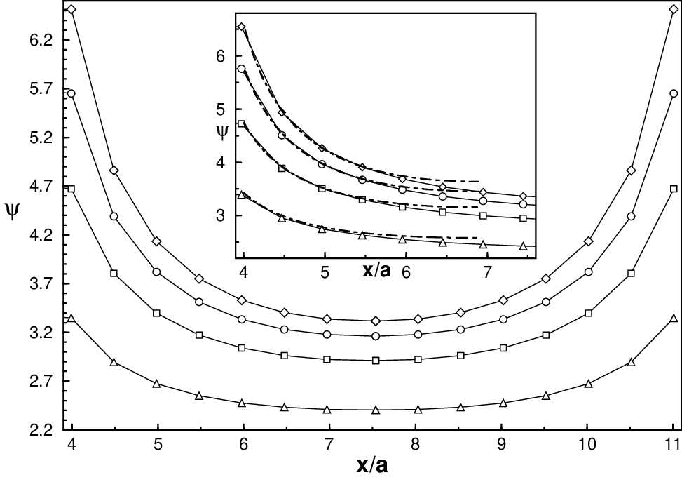
The idea of charge renormalization has originally been proposed for a cell model [Alexander:JCP80-84-5776], where only a single Wigner-Seitz cell of the colloidal crystal is considered. To facilitate solution of the PB equation, furthermore the complicated geometry of the true Wigner-Seitz cell is replaced by a sphere. The predictions of the spherical cell model for the effective parameters and (dash-dotted lines in Fig. 8) agree very well with the values obtained from the full numerical calculation (symbols). Again, there is no significant dependence on the crystal structure indicating the absence of many-body effects.
A more direct comparison to the cell model can be made by looking at the electrostatic potential itself. In Fig. 9 the numerical result for the potential along a line between two out of 108 macroions in an FCC configuration is shown for several values of the bare charge (symbols). The agreement to the spherical cell model result (dash-dotted line) is very good, except near the cell edge, where the spherical approximation leads to a higher value of the potential in the cell model. This is due to the fact that the half-width of the actual FCC Wigner-Seitz cell in the direction shown is while the size of the spherical cell with equal volume is only .
6.4 Melting Point

Finally, we take a look at a macroscopic property of the suspension obtained from a full dynamical calculation, namely the melting point. For systems of point-like Yukawa particles this quantity is known from the classic work of Robbins, Kremer, and Grest [Robbins:JCP88-88-3286]. In this work, the melting line has been calculated from a molecular dynamics simulation by using the Lindeman criterion stating that melting occurs whenever the root mean square displacement exceeds the value of 19% of the mean distance between macroions. The result is
| (42) |
in terms of the parameters
| (43) | |||||
| (44) |
The former is simply the inverse effective screening length scaled with the mean particle distance. The latter represents a scaled temperature ( in units of the Einstein phonon energy) which is related to the strength of the interaction defined in Eq. (39) and, hence, the effective charge . The function depends on the lattice-type of the crystalline phase and is given in Tab. I of Ref. [Robbins:JCP88-88-3286].
In Fig. 10 we show the mean square displacement, , of the macroions as a function of time as calculated from the combined PB–Brownian dynamics method. By using the effective force parameters and from the previous section, the values of and can be calculated so that a comparison to Eq. (42) becomes possible. The value of is practically independent of the bare charge . The effective temperature, in contrast, depends strongly on with values shown next to each curve in Fig. 10. The Lindemann value is reached for , so that by the same criterion as in Ref. [Robbins:JCP88-88-3286] the colloidal crystal melts around . The melting occurs quite close to the saturated value of the effective charge. The corresponding effective temperature cannot be exceeded for our system. We conclude that our estimate of the melting point is in reasonable agreement with the value obtained by Robbins et al. in Ref. [Robbins:JCP88-88-3286] for Yukawa systems.
7 Discussion
The physics of charge stabilized colloidal suspensions poses challenging problems resulting from the presence of many coupled degrees of freedom. A treatment has been possible so far only in limited regions of parameter space either due to the necessity of approximations in analytical treatments or because of practical limitations in numerical simulations. We have here described in detail a method which makes accessible the regime of large macroionic charge, low salt concentration, and relatively high colloid volume fraction, where many-body interactions between the macroions become important [Dobnikar:NN1-02, Dobnikar:NN2-02]. This has been achieved by combining a Poisson-Boltzmann field description of the small ions with a Brownian dynamics simulation of the charged colloidal particles. By describing the small ions in terms of a continuous density, the computational effort becomes independent of their number. In this way, the main limitation, which precludes the application of primitive model simulations to the above parameter regime is circumvented. At the same time, in contrast to analytical treatments like linearized DLVO theory or cell models, macroionic many-body effects are fully accounted for in our approach.
In the present work, we have focused on the case where the effective interactions are still of a pairwise additive Yukawa form. By comparing our simulation results to linearized DLVO theory and cell model calculations, which are applicable in this regime, the method has been thoroughly validated. Furthermore, its potential applications have been illustrated which reach beyond simple structural calculations [Fushiki:JCP97-92-6700, Lowen:JCP98-93-3275] and also include the evaluation of thermodynamic properties, e.g. the phase behavior of charged colloidal suspensions. These applications are pursued in greater detail elsewhere [Dobnikar:NN4-02].
Directions for further development from a physical viewpoint are twofold. First, on the Poisson-Boltzmann level of description correlations between the small ions are neglected, which limits the applicability to monovalent small ions and small coupling . The range of applicability could be extended by using more elaborate density functional theory similar to Refs. [Lowen:JCP98-93-3275, Lowen:EL23-93-673]. Secondly, the calculation of rheological properties necessitates inclusion of hydrodynamic effects. The framework of a field description of the solvent on which our approach is built, readily accommodates such an extension as well [Shyy:CTCTP-97].
Desirable improvements of the computational efficiency include parallelization of the method and the implementation of more sophisticated solvers for the discrete equations. Several possibilities for the latter have been compared in Ref. [Holst:JCoC16-95-337] where a combination of inexact Newton and multigrid methods was found to be the most efficient. A parallelization strategy that naturally fits together with the use of the overset spherical grids is to use a domain decomposition approach [Smith:DD-96] also for the Cartesian background grid. Developments along these lines are currently pursued.