Fermionic renormalization group methods for transport through inhomogeneous Luttinger liquids
Abstract
We compare two fermionic renormalization group methods which have been used to investigate the electronic transport properties of one-dimensional metals with two-particle interaction (Luttinger liquids) and local inhomogeneities. The first one is a poor man’s method setup to resum “leading-log” divergences of the effective transmission at the Fermi momentum. Generically the resulting equations can be solved analytically. The second approach is based on the functional renormalization group method and leads to a set of differential equations which can only for certain setups and in limiting cases be solved analytically, while in general it must be integrated numerically. Both methods are claimed to be applicable for inhomogeneities of arbitrary strength and to capture effects of the two-particle interaction, such as interaction dependent exponents, up to leading order. We critically review this for the simplest case of a single impurity. While on first glance the poor man’s approach seems to describe the crossover from the “perfect” to the “open chain fixed point” we collect evidence that difficulties may arise close to the “perfect chain fixed point”. Due to a subtle relation between the scaling dimensions of the two fixed points this becomes apparent only in a detailed analysis. In the functional renormalization group method the coupling of the different scattering channels is kept which leads to a better description of the underlying physics.
pacs
71.10.-w, 71.10.Pm, 73.21.Hb1 Introduction
The sensitivity of one-dimensional (1D) correlated electron systems – so called Luttinger liquids (LL) [1] – to local single-particle inhomogeneities (e.g. a single impurity) leading to a (back-) scattering of electrons with momentum transfer (with being the Fermi momentum) was recognized several decades ago [2, 3, 4, 5]. The density-density response function at zero frequency shows a power-law singularity when the momentum transfer approaches with an exponent determined by the Luttinger liquid parameter (for repulsive interactions; in the noninteracting case). It was computed for a specific field-theoretical model – the Tomonaga-Luttinger (TL) model – after mapping the interacting fermionic problem onto a free bosonic Hamiltonian using the bosonization method [6]. The TL model is known to describe the low-energy physics of a large class of 1D metals [1].
At the beginning of the 90’s it became apparent that the realization of sufficiently well defined 1D quantum wires and thus the possibility to experimentally investigate LL physics would only be a matter of a few more years of research. This was one of the reasons for a renewed theoretical interest in such systems. The understanding of the role of local impurities was further sharpened by renormalization group (RG) studies within the bosonized model [7, 8]. In these studies the TL model was supplemented in two ways. In a first step a term solely describing the to (and vice versa) backscattering (of amplitude ) was added to the Hamiltonian. Using bosonization this leads to a term , with being the bosonic field and the position of the impurity. The resulting field-theoretical model is known as the local sine-Gordon model. In a RG procedure perturbative in it was shown that grows and is thus a relevant perturbation (for repulsive interactions with ). At a sufficiently low energy scale the perturbative RG breaks down. In a second step the opposite case of two semi-infinite TL chains with a weak link of amplitude was studied. This was shown to scale to zero. Based on these insights and an exact solution at it was speculated that for repulsive interactions even a weak single impurity will scale towards the strong impurity limit implying that at low energies observables show power-law scaling with exponents characterized by the scaling dimension of the “open chain fixed point” . E.g. the local spectral function close to the impurity will vanish as and the conductance across the impurity as
| (1) |
with being the temperature. For small the corrections to “perfect” conductance [9] are given by the scaling dimension of the (unstable) “perfect chain fixed point”,
| (2) |
Within the local sine-Gordon model the above conjecture was later confirmed using numerical [10] and exact [11] methods.
The physics of spinless inhomogeneous LLs and systems with spin is quite similar in many respects and for simplicity we here mainly focus on the spinless case. The scaling exponents just given are slightly different if the spin is included. Towards the end of this article we briefly explain how the spin can be included in the two fermionic RG approaches described here and discuss a novel feature which results from it.
In parallel to the bosonization approach a fermionic poor man’s RG method was developed which does not rely on the mapping onto a bosonic field theory [12]. In this approach the single-particle impurity scattering problem is first solved exactly within the 1D electron gas model. Next, the Hartree and Fock terms [leading order perturbation theory in the two-particle interaction ] are computed with the scattering states. The Hartree diagram produces a potential term which oscillates as , decays as , and has a prefactor given by the reflection amplitude of the (bare) impurity. Scattering off the Hartree potential leads to a logarithmically diverging correction to the transmission amplitude if
| (3) |
where is a characteristic spatial scale of the interaction and
| (4) |
is the relevant amplitude of the (Fourier transform of the) interaction, with being the Fermi velocity. The authors argue that one can iterate this procedure and produce divergent terms of higher order .
To resum these terms a real space RG method is suggested. At scale the scattering potential is considered only for with a spatial cutoff . This way the logarithmic divergence is regularized. Then the region with its renormalized reflection and transmission amplitudes is viewed as an effective barrier from which the Hartree potential and the Fock term for the region outside can be computed. One next considers and iterates the above steps. This leads to a single differential equation for the transmission amplitude at momentum . For the following analysis it is essential to note that the nontrivial spatial dependence of the scattering potential at each step is and does not change during the RG procedure.
It was argued that, in contrast to the bosonic RG method which is perturbative in the impurity strength, this fermionic procedure, although being applicable only for sufficiently small (weak two-particle interaction), can be used to describe the full crossover from the weak to the strong impurity limit. Further down we challenge this statement. A detailed analysis for the single impurity case shows that the poor man’s approach heavily relies on a subtle relation between the scaling dimensions of the “perfect” and “open chain fixed points”. The method is commonly regarded as being very intuitive and has been generalized to study transport through two barriers (resonant tunneling) [13, 14], through Y-junctions of three LLs [15], and through regular networks of LLs [16] as well as transport across a LL-superconductor junction [17]. Remarkably, the lack of a formal framework from which the poor man’s flow equations can be deduced led to a dispute about their correct form for the double barrier case [13, 14].
In both the fermionic RG as well as the field-theoretical description only the scaling of the backscattering amplitude (and vice versa) was considered. Undoubtedly the backscattering component of a general scattering potential with matrix elements is (i) the one which grows the fastest when the infrared cutoff is lowered and is (ii) the component which at the end of the RG flow determines the conductance across the impurity. But in more elaborate RG procedures all scattering channels will couple and also the amplitudes with , not equal to will grow. Even if the matrix elements with momentum transfer different from are absent in the original Hamiltonian generically they will be generated during the RG procedure. One might speculate that this feedback will lead to intermediate fixed points not captured by the local sine-Gordon model (as no other matrix elements than are kept in the model) and the poor man’s RG (as the feedback is neglected). Motivated by this reasoning an alternative fermionic RG procedure was developed starting from the rather general functional RG (fRG) framework [18, 19]. It allows for a description of the full functional form of the renormalized effective impurity potential. Using truncated fRG flow equations it was shown that indeed no intermediate fixed points are realized [20, 21, 22]. As a further advantage this RG method can directly be applied to microscopic lattice models and does not require a mapping onto the 1D electron gas or an effective field theory. It is rather straightforward to extend the fRG approach to study resonant transport through a double barrier [22], transport through a wire with three and four impurities [23], and junctions of more than two LLs [24, 25].
In the fRG formalism one derives an infinite hierarchy of coupled differential flow equations for the cutoff dependent one-particle irreducible vertex functions. In practical applications this hierarchy must be truncated. To study the physics of local inhomogeneities in spinless LLs up to leading order in the two-particle interaction it is sufficient to keep the flow of the frequency independent self-energy (one-particle vertex) [20]. The quantitative agreement to the results derived by bosonization in the limits of weak and strong impurities as well as to numerical results obtained for small systems can be improved if the flow of the static part of the effective two-particle interaction (two-particle vertex) is kept [21, 22]. Details are given below. The frequency independent self-energy can be interpreted as an effective, renormalized impurity potential. For strong bare impurities it spatially oscillates with frequency and decays as the inverse distance from the inhomogeneity up to a scale , beyond which it dies off exponentially. Scattering off this effective impurity then leads to the power-law decay of the conductance as a function of . For weak bare impurities and not too low temperatures the oscillatory effective potential only decays with exponent . For lower temperatures a crossover to the strong impurity behavior can be observed and the system flows to the “open chain fixed point”.
Below we give more details on the truncated fRG procedure and the basic equations for the poor man’s RG (Sec. 2). We discuss the most important results and compare the outcomes of the two fermionic RG approaches (Sec. 3). It is shown that the truncated fRG can be used to describe the full crossover from the weak to the strong impurity limits while the poor man’s RG seems to have difficulties close to the “perfect chain fixed point”. We show that a single RG equation – as derived in the poor man’s RG for the effective transmission at momentum – is in general not enough to describe the crossover behavior. We then briefly comment on how the spin degree of freedom is included in both methods (Sec. 4). Finally, the comparison of the two fermionic RG methods for the single impurity case is summed up and briefly extended to Y-junctions of three LLs (Sec. 5). In the Appendix we discuss the additional approximations necessary to derive the poor man’s RG equation within the fRG framework.
2 The methods
In this section we present the basic equations of the fRG approach and the poor man’s RG. We focus on the simplest situation of a single impurity in an otherwise “perfect” chain which is coupled “adiabatically” to two semi-infinite noninteracting leads [9].
2.1 The functional RG approach
The fRG was recently introduced as a powerful new tool for studying interacting Fermi systems [18]. It provides a systematic way of resumming competing instabilities and goes beyond simple perturbation theory even in problems which are not plagued by infrared divergences. In our application the interacting quantum wire will be coupled to noninteracting leads as it is the case in systems which can be realized in experiments. The leads are modeled as 1D tight-binding chains with hopping matrix element . As we are interested in the effect of a single impurity in the bulk part of the wire and not the role of the contacts the latter are modeled as being perfect, that is the conductance through the interacting system of length in the absence of the impurity is (up to our numerical accuracy). This implies that the interaction must be turned on spatially smoothly close to the contacts (“adiabatic contacts”) [22, 9]. Before setting up the fRG scheme we integrate out the noninteracting leads using a standard projection technique so that we only have to deal with an interacting system of size [22]. The energy scale related to the length of the interacting part will provide an infrared cutoff for power-law scaling as a function of other energy variables.
In the fRG procedure the noninteracting propagator is replaced by a propagator depending on an infrared cutoff . Specifically, we use
| (5) |
with running from down to . The cutoff function is chosen such that the fermionic Matsubara frequencies are cut out (for details see the Appendix A of Ref. [26]). Note that contains the frequency dependent self-energy contribution from the leads
| (6) |
with indicating the lattice site and the filling -, interaction -, and -dependent chemical potential . It is chosen such that the entire system (wire and leads) has the desired filling at any and . Using in the generating functional of the irreducible vertex functions and taking the derivative with respect to one can derive an exact, infinite hierarchy of coupled differential equations for the vertex functions, such as the self-energy and the irreducible two-particle interaction . In particular, the flow of the self-energy (one-particle vertex) is determined by itself and the two-particle vertex, while the flow of is determined by , , and the flowing three-particle vertex . The latter is computed from a flow equation involving the four-particle vertex, and so on. At the end of the fRG flow is the self-energy of the original, cutoff-free problem we are interested in. A detailed derivation of the fRG flow equations for a general quantum many-body problem which only requires a basic knowledge of the functional integral approach to many-particle physics and the application of the method for a simple problem are presented in Ref. [19].
In practical applications the hierarchy of flow equations has to be truncated and only provides an approximation for the exact . As a first approximation we neglect the three-particle vertex. The contribution of to is small as long as is small, because is initially (at ) zero and is generated only from terms of third order in . Furthermore, stays small for all if the bare interaction is not too large. This approximation leads to a closed set of equations for and [22].
We here do not give these equations but instead implement a second approximation: the frequency dependent flow of the renormalized two-particle vertex is replaced by its value at vanishing external frequencies, such that and hence remains frequency independent. Since the bare interaction is frequency independent, neglecting the frequency dependence leads to errors only at second order for the self-energy, and at third order for the two-particle vertex at zero frequency. For the approximate flow equations we then obtain
| (7) |
and
| (8) |
where the lower indexes , , etc. stand for the single-particle quantum numbers of the chosen basis (e.g. the Wannier basis or the momentum state basis) and
| (9) |
The abbreviation stands for taking the positive as well as negative Matsubara frequency with absolute value closest to at fixed . At the initial cutoff the flowing two-particle vertex is given by the antisymmetrized interaction and the self-energy by the single-particle terms of the Hamiltonian not included in , e.g. the impurity.
Next we specify our model for the interacting LL wire with noninteracting leads. We use the 1D tight-binding model with nearest-neighbor hopping and nearest-neighbor interaction . It is given by
| (10) | |||||
where we used standard second-quantized notation with and being creation and annihilation operators on site , respectively and the local density operator . The filling and interaction dependent real number must be determined iteratively such that at fixed common (for the leads and the wire) the interacting wire has the desired filling. For the mostly studied case of half-filling particle-hole symmetry implies . As mentioned above the interaction is turned on and off smoothly over a small fraction of the interacting lattice sites. The constant bulk value is denoted by .
The homogeneous model with a constant interaction across all bonds can be solved exactly by the Bethe ansatz [27]. It shows LL behavior for all particle densities and any interaction strength except at half filling for . The - and -dependent LL parameter can be determined solving coupled integral equations [27], which in the half-filled case can be done analytically with the result
| (11) |
for . As depends on the filling it is essential to tune the interacting wire to the desired filling by choosing the appropriate [see Eq. (10)]. Only then a comparison of the fRG results to the ones obtained by bosonization is possible.
The Hamiltonian (10) is supplemented by an impurity part
| (12) |
where is a static potential. Local site impurities of amplitude at are given by a potential
| (13) |
and local hopping impurities with hopping across the link by
| (14) |
In our RG procedure we parameterize the static real space vertex by a flowing nearest-neighbor interaction
| (15) |
We furthermore neglect the feedback of the self-energy on the flow of . The differential equation for the renormalized bulk interaction is then determined after transforming Eq. (15) to momentum space and fixing the momenta on the Fermi surface [28]. It reads (in the limit )
| (16) |
with
| (17) | |||||
where stands for the fermionic Matsubara frequency closest to . The initial condition is . The bond dependent renormalized interaction follows from the bulk by multiplying with . After performing these additional approximations the flow equations for the Wannier basis matrix elements of the self-energy read
| (18) |
All other components vanish. The self-energy enters also the right-hand side of these equations via the full propagator . The initial conditions at are
| (19) |
At the end of the fRG procedure the diagonal part of the approximate self-energy can be interpreted as an effective impurity potential, while is the renormalized hopping.
For general parameters the set of coupled differential equations can only be solved numerically. This can be done for fairly long chains (up to lattice sites) as computing the right-hand side of the flow equations only requires the tridiagonal part of the inverse of a tridiagonal matrix which can be obtained in order time [28]. In the limiting cases of weak and strong impurities and neglecting the flow of the two-particle interaction altogether the flow equations can be solved analytically at . This is discussed in Sec. 3.
The truncated fRG procedure provides an approximation for the self-energy and thus via the Dyson equation an approximation for the interacting one-particle Green function . If the inelastic (frequency dependent) processes the two-particle interaction generates are neglected, the conductance can be computed from the matrix element of the retarded Green function by a generalized Landauer-Büttiker formula [22]
| (20) |
where is the Fermi function, the band width ( for ), and
| (21) |
the effective transmission. Because of the frequency independence of the analytic continuation of to the real axis, necessary to obtain , is straightforward. During the RG procedure the self-energy and thus the propagator acquire additional dependencies on the temperature and on the energy scale .
Inelastic processes vanish in the limit . For they are absent in our approach as we assumed the self-energy to be frequency independent and using Eq. (20) is thus consistent with our earlier approximations – it presents no further approximation. In general inelastic processes lead to corrections to Eq. (20) of order and higher. It is important to note that inelastic processes due to the two-particle interaction are also neglected in the poor man’s RG as well as in the bosonization approach. In the latter they are disregarded because the bulk part of the local sine-Gordon model corresponds to the TL model in which all infrared RG irrelevant terms such as umklapp scattering are left out. At finite scales such terms imply inelastic scattering.
2.2 Solution of the poor man’s RG equation
The basic idea of the poor man’s RG was already presented in the introduction. It is set up for the 1D electron gas model. The method leads to the flow equation [12]
| (22) |
for the transmission at , with and introduced in Sec. 1. It only depends on a single energy scale, the infrared energy cutoff , which must be contrasted to the fRG approach in which the scales , , and appear. The integration of Eq. (22) starts at the ultraviolet cutoff with the initial condition , where is the bare transmission. To obtain the energy or temperature dependence of the renormalized transmission the integration is stopped at or , respectively. The assumed dependence on only one energy scale implies that the variable one is interested in must be much larger than all the other scales. In the fRG in contrast the interplay of the scales , , and can be studied. The solution of Eq. (22) is
| (23) |
where must be substituted by the energy variable of interest (e.g. ). The bare reflection probability is denoted by . The expression for the conductance follows after multiplying the transmission (probability) by .
For the upcoming analysis it is important to note that the leading order contribution of for the 1D electron gas model with two-particle interaction is given by [1]
| (24) |
with the forward- [] and backward-scattering [] amplitudes.
3 A comparison of results for the conductance and the renormalized impurity potential
In this section we compare the results for the conductance and the renormalized impurity potential obtained using the two fermionic RG methods. We start with the two limits of weak and strong bare impurities.
3.1 The conductance for weak and strong impurities
The solution Eq. (23) of the poor man’s RG equation can easily be expanded in the limits of weak () and strong () bare impurities. In the first case this gives
| (25) |
while in the second one finds
| (26) |
Within the bosonization approach the two relevant scaling exponents are give by and [see Eqs. (2) and (1)]. With Eq. (24) one finds
| (27) |
to leading order in the two-particle interaction and Eqs. (25) and (26) are consistent with the bosonization results Eqs. (2) and (1) if is replaced by . One is thus tempted to conclude that the poor man’s RG result Eq. (23) describes the full crossover from the “perfect chain fixed point” to the “open chain fixed point” as long as the interaction remains small . Below we argue that the analytic Breit-Wigner form Eq. (23) is incomplete and that the apparent agreement with the bosonization result heavily relies on the subtle relation Eq. (27) (which can be traced back to what is called “duality” in the field-theoretical approach).
In the two limits considered in the present subsection also the fRG flow equations can be tackled analytically provided that the flow of the effective nearest-neighbor interaction is neglected. In Ref. [20] it was shown that at for weak bare impurities
| (28) |
rather independently of the model considered (that is not only for the lattice model with nearest-neighbor interaction and independent of the type of impurity considered). Within the Born approximation of single-particle scattering theory the transmission (conductance) can be obtained from the backscattering amplitude . Assuming that in Eq. (28) can be replaced by the scale (as it is routinely done in the poor man’s RG; see above) the transmission shows the correct scaling behavior with an exponent which agrees to the bosonization result to leading order in the two-particle interaction. In Ref. [20] it was also shown that at , for the lattice model described above, and for a strong hopping impurity (weak link) the local spectral function close to the impurity shows power-law scaling (as a function of energy) with an exponent equal to that found for an open chain. The latter agrees to leading order with the bosonization exponent . Following standard arguments (Fermi’s Golden Rule) [7] one can then conclude that the conductance at low energy scales shows power-law scaling with an exponent which agrees to leading order with the bosonization result .
3.2 The generalized Breit-Wigner form of the transmission
The expressions (20) and (21) for the transmission (conductance) used at the end of the fRG procedure can be brought into a form similar to that of the poor man’s RG Eq. (23). To be specific we consider a site impurity at (in the bulk of the interacting wire) of amplitude . In a first step one runs the fRG flow down to and determines the approximate self-energy . Denoting the single-particle version of the noninteracting part of the Hamiltonian by , the matrix
| (29) |
forms an effective single-particle “Hamiltonian”, which is non-hermitian because of the leads contribution Eq. (6) . After setting the renormalized hopping matrix element from site to site to zero, that is after cutting the chain in two parts, we define an auxiliary Green function [resolvent matrix of size ]
| (30) |
Via the auxiliary Green function still contains information about all system parameters, in particular and : . Within the framework of single-particle scattering theory and using a standard projection technique [22] the effective transmission can be written as
| (31) |
with
| (32) |
real functions and , and the renormalized energy of the impurity site , . If we now consider and plug Eq. (31) into the generalized Landauer-Büttiker formula (20) we end up with
| (33) |
Using as our scaling variable this generalized Breit-Wigner form is similar to that of Eq. (23) obtained within the poor man’s RG. Using the energy related to the inverse size of the interacting part of the system as an energy scale is valid also in the poor man’s RG according to the construction of the RG equation. The characteristic difference of the two approaches is the absence of a scale dependence in the first term of the denominator of Eq. (23). This will become crucial in the following.
To further develop the relation between the two generalized Breit-Wigner forms we next analyze the scaling properties of and . In Fig. 1 results for and obtained by numerically solving the truncated fRG flow equations for strong [Fig. 1(a)] and weak [Fig. 1(b)] bare impurities are shown on a log-log scale. The parameters are and , , [Fig. 1(a)] and [Fig. 1(b)], and the size of the interacting wire varies from to . For strong bare impurities is constant, while the imaginary part of the auxiliary Green function shows power-law scaling as a function of . As the imaginary part can be neglected in the denominator of Eq. (33). From this one concludes that the exponent of is twice as large as that of . The exponent extracted from the fRG data for [see Fig. 1(a)] agrees to leading order in with the expected result , with taken from Eq. (11) [22]. For weak bare impurities is constant while follows a power law. Furthermore, and the conductance Eq. (33) can be expanded in this ratio. From this expansion one concludes that the correction of the conductance to scales with twice the exponent of . The exponent of [see Fig. 1(b)] determined numerically indeed agrees to leading order with the expected one [22].


It is important to note that for Eq. (33) provides the exact analytical form of the conductance even if one goes beyond the fRG truncation used here. We expect that if computed exactly and show power-law scaling with the bosonization exponents (not only the leading order exponents) in the corresponding limits of weak and strong impurities.
Identifying and might appear ambiguous as one can devide the numerator and denominator of Eq. (33) by the scale dependent part of and end up with a function similar to Eq. (23) in which the first term in the denominator is scale independent. However, the above relations become unique if one considers the finite generalization of Eq. (23) as given in Eq. (5) of Ref. [13] which must be compared to Eq. (31).
These insights provide hints that the absence of the scale dependence in the first term of the denominator of Eq. (23) (the “real part”) constitutes a problem for the poor man’s RG in the limit of weak bare impurities. In fact, in the poor man’s RG approach the “imaginary part” carries the scaling in both limits of weak and strong impurities. The observation that Eq. (23) reproduces the bosonization results in both limits thus relies heavily on the fact that to leading order in the two-particle interaction. This is different in the fRG approach, in which two different functions carry the scaling properties in the two limits. The analysis also reveals that for a method that leads to a generalized Breit-Wigner form one needs at least two independent RG equations (one for the real and one for the imaginary part of ) to fully describe the crossover.
3.3 The one-parameter scaling function
We now further elaborate on the differences of the two fermionic RG approaches by studying the one-parameter scaling properties of the conductance (transmission).
That the full crossover from the weak to the strong impurity limit within the local sine-Gordon model follows a one-parameter scaling function was shown analytically in Ref. [7] for . Within this model it was later confirmed for other LL parameters [10, 11] and generalized to microscopic models in Refs. [21] and [22]. The scaling ansatz is given by [7]
| (34) |
with the nonuniversal scale and being or . For appropriately chosen the curves for different (but fixed ) can be collapsed onto the -dependent scaling function . It has the limiting behavior for and for . For the following it is important to note that using either Eq. (11) or Eq. (24) the large exponent has a contribution that is linear in the two-particle interaction. It follows from taking the “open chain fixed point” exponent (large behavior) and dividing by half the exponent of the “perfect chain fixed point” which by convention was explicitly taken into account in the definition of the variable [see Eq. (34)].
Achieving the form Eq. (34) for the result of the poor man’s RG Eq. (23) is straightforward. The scaling variable is and the scaling function
| (35) |
Independent of the strength of the two-particle interaction it is thus given by the noninteracting scaling function . While the behavior at small is reproduced correctly, for large , decays . This can be traced back to the fact that within the poor man’s RG the weak and strong impurity exponents are both strictly linear in the two-particle interaction and have the same modulus. As mentioned above the correct large exponent has a contribution linear in the two-particle interaction.

In Fig. 2 we show conductance data obtained numerically from the fRG procedure at a fixed small and for temperatures . For appropriately chosen the data for different and , (open symbols) fall onto a single curve. The different symbols and colors indicate different . A similar collapse is found for and [21]. In the definition of [see Eq. (34)] we used the fRG approximation for (for and , ). The same can be found at filling for . Data for these parameters are shown as the filled symbols in Fig. 2. The collapse confirms that the one-parameter scaling function indeed only depends on and not on and separately.
In contrast to , depends on and for large shows a power-law decay with an exponent different from (see the black line in Fig. 2). In the fRG approximation the two exponents and are determined numerically from the temperature dependence of the conductance for weak and strong bare impurities (or, with the same result, as described in the last subsection). In contrast to the poor man’s method they have higher (than leading) order corrections and the -dependent part does not cancel if the scaling ansatz is applied. In fact, as shown in Figs. 5 and 7 of Ref. [22] the bosonization and fRG exponents agree well beyond the linear regime in the limits of weak and strong impurities, even though formally only the leading order Taylor coefficients are the same (as terms of order and higher are only partially kept in the truncated fRG scheme). In the light of these observations it is interesting to ask whether the fRG approximation of the ratio , that is the large decay exponent of the scaling function, has the correct leading order (in ) behavior. Unfortunately, the numerical accuracy of the data for the two exponents is not high enough to make definite statements about this. For small (that is in the linear regime of ), both exponents are small and any small error (in particular of the denominator) will lead to an inaccurate ratio. For close to 1, for which the truncated fRG works best, the complete form of the scaling function (beyond the two limits and ) is not known analytically within the local sine-Gordon model, and no direct comparison with the fRG approximation is possible. But even for , the largest LL parameter (that is the smallest two-particle interaction) for which was computed in the field-theoretical model, the fRG data of our lattice model are surprisingly close to the curve obtained using bosonization as shown in Fig. 4 of Ref. [21]. In this respect the fRG method goes significantly beyond the poor man’s approach.
3.4 The decay of the effective, renormalized impurity potential
It seems to be possible to understand the problems of the poor man’s RG close to the “perfect chain fixed point” in terms of the real space properties of the effective impurity potential. As described in the introduction in the construction of the poor man’s RG equation the effective impurity potential always decays as the inverse distance from the impurity, while the prefactor is renormalized. This holds up to the spatial scale set by the infrared cutoff (e.g. the temperature ) and regardless of the strength of the bare impurity. Using the fRG approach we now show that this is correct for strong bare impurities and on asymptotically small scales. For weak bare impurities and on large to intermediate scales the renormalized impurity potential decays more slowly, an observation which can also be related to the results known from bosonization.

In Fig. 3 fRG results for the decay of the oscillatory part of away from for a strong bare impurity at different are shown. Here we used a hopping impurity with , that is a hopping across the bond which is only 10% of the hoppings across all other bonds. Generically, for the lattice model under consideration, both the diagonal and off-diagonal parts of show decaying oscillations. For symmetry reasons (particle-hole symmetry) for half-filling and hopping impurities, as chosen in Fig. 3. The figure clearly shows that up to a scale beyond which the oscillation decays exponentially. For more general parameters and strong bare impurities shows the same characteristics. This result is in agreement with the reasoning leading to the poor man’s RG equation.

In Fig. 4 we show the effective exponent for the decay of the oscillations of as a function of the distance from a site impurity of different strengths obtained at (dashed) and (solid). For weak bare impurities and on intermediate scales the effective impurity potential follows a power-law decay with a -dependent effective exponent (see the plateau at value for at ). Only for larger distances and lower temperatures, that is on lower-energy scales, or for stronger bare impurities this behavior crosses over to the strong impurity limit with decay exponent . This behavior seems not to be included in the poor man’s approach. The steep rise of the effective exponent on a scale indicates the crossover to exponential decay (see Fig. 3). The off-diagonal component of the self-energy shows similar behavior.
When studied as a function of the effective exponent at the weak impurity plateau is found to be close to . This exponent can be related to the results known from bosonization. For weak impurities and on large to intermediate energy scales the effective impurity stays small and is approximately . To obtain the reduction of the transmission with respect to 1, one can then treat the renormalized impurity potential within the Born approximation. This requires the component of the impurity potential. Fourier transforming the above potential leads to and finally to , that is the scaling behavior known from the local sine-Gordon model.
4 Including the spin degree of freedom
Both fermionic RG methods were extended to study inhomogeneous LLs with spin. Within the generalization of the local sine-Gordon model to the case with spin the physics is in many respects similar to that of spinless inhomogeneous LL. The system is characterized by the “perfect” and the “open chain fixed points” with scaling dimensions and , respectively [7, 8]. We here assume a spin-rotationally invariant interaction. From the scaling dimensions the exponents of the power-law corrections to the fixed-point conductance and the exponent of the local spectral weight follow as in the spinless case.
To obtain the scaling exponents to first order in the two-particle interaction within fermionic RG methods it is essential to keep the flow of the static two-particle vertex (the effective interaction). As it is known from the so called g-ology analysis for homogeneous LLs the backscattering component between electrons with opposite spin flows to zero if the infrared cutoff is lowered [29]. In the poor man’s RG the flow equation for the transmission at momentum was supplemented by the g-ology RG equations for the static two-particle vertex of a homogeneous TL model. This way the prefactor in Eq. (22) becomes -dependent. For strong bare impurities a new feature appears. If for the two-particle interaction , that is for repulsive interactions with a sizable bare backscattering component, the conductance across a single impurity first increases as a function of the energy scale before it is suppressed on asymptotically small scales. This effect is not captured within the local sine-Gordon model.

The fRG approach was generalized to the extended Hubbard model with local interaction and nearest-neighbor interaction [26]. In a wide range of parameters – to which we stick in the present context – this model shows LL behavior. The flow equations for the different components of the static two-particle vertex go beyond the g-ology approximation (see Figs. 2 and 3 of Ref. [26]), but the feedback of the inhomogeneity on the flow of the vertex (via the self-energy) is neglected. As shown in Fig. 5 also within the fRG approach for a strong site impurity the conductance first increases when the temperature is lowered before the asymptotic power-law suppression sets in. For the extended Hubbard model, , which can be positive or negative for , depending on the density and the relative strength of the two interaction parameters. At quarter-filling , is negative and therefore leads to an enhanced conductance for . In case of a negative the crossover scale is given by
| (36) |
and becomes exponentially small for weak interactions. For the conductance increases as a function of decreasing down to the lowest temperatures shown in Fig. 5. For increasing nearest-neighbor interactions a suppression of at low becomes visible, but in all the data obtained at quarter-filling it is much less pronounced than what one expects from the asymptotic power law with exponent . By contrast, the suppression is much stronger and follows the expected power law more closely if parameters are chosen such that the bare two-particle backscattering becomes negligible, as can be seen from the conductance curve for and (magenta) in Fig. 5. The value of [26] for these parameters almost coincides with the one for another parameter set in the plot, and (blue triangles), but the behavior of is completely different. Note that at the scaling is cut off as can be seen at the low end of the magenta curve in the figure. The scaling exponents (if accessible, as e.g. for the magenta curve) extracted from the - or -dependence of the conductance (for weak and strong bare impurities) as well as the exponent extracted from the -dependence of the local spectral function agree to leading order in the two-particle interaction with the bosonization results.
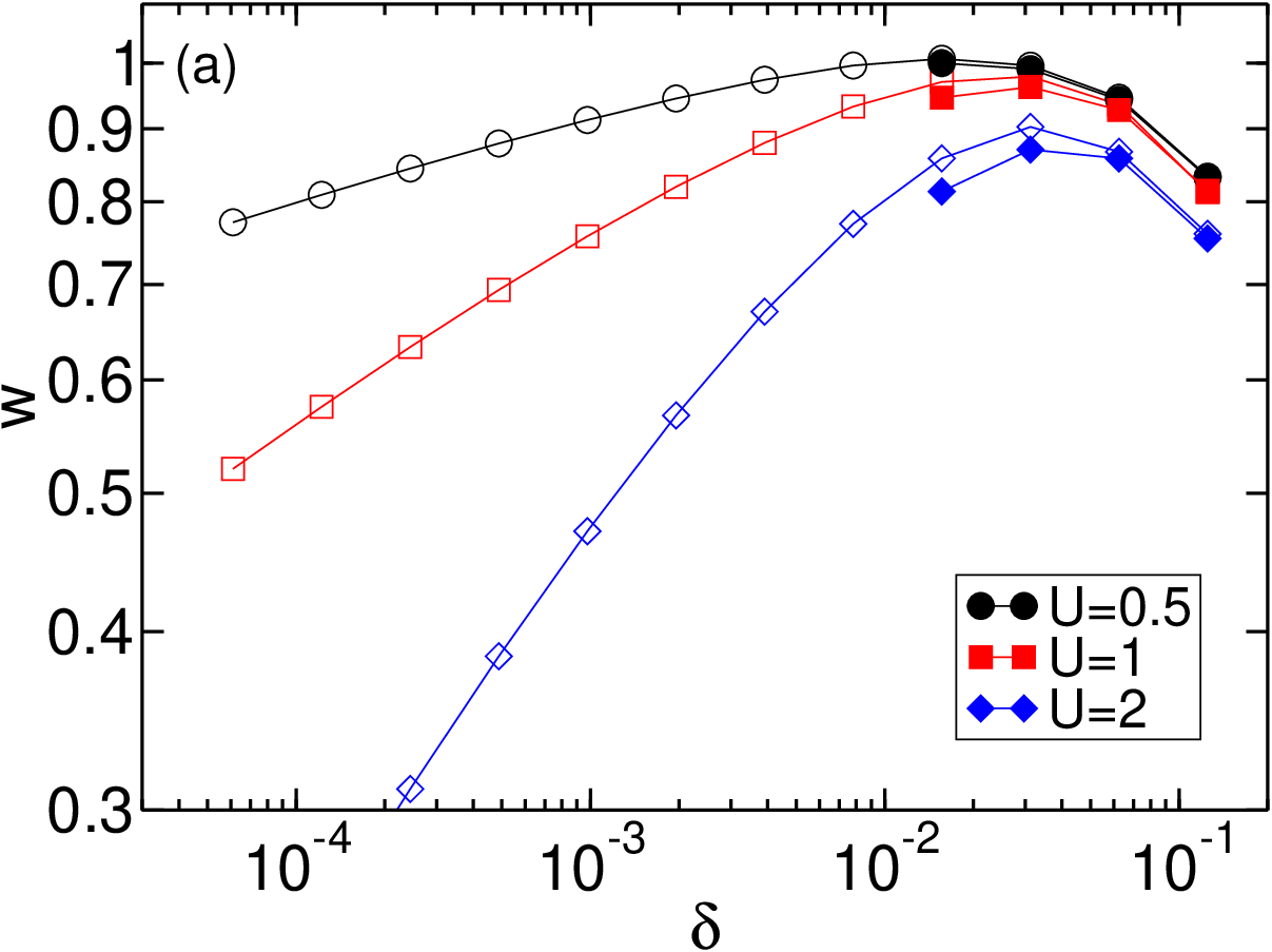

Using the fRG we are in a position to even address very subtle questions such as how accurately the crossover scale is reproduced by the truncated procedure. To this end we need exact or numerically exact data to compare our fRG results with. As no such data are available for the conductance of the extended Hubbard model with a local impurity we compute the spectral weight at , close to the impurity, and at as a function of for this model and compare it to very accurate numerically obtained density-matrix renormalization group (DMRG) data [30]. We here decouple the leads (as they are not included in the standard DMRG approach) and study a finite system of length . In Fig. 6 we present fRG and DMRG results for taken at site for a hopping impurity with , , different , and [Fig. 6(a); small backscattering] as well as [Fig. 6(b); sizable backscattering]. The spectral function close to the impurity site and the spectral weight show a similar crossover behavior as [see Fig. 6(b)]. For parameters at which the bare two-particle backscattering is small as in Fig. 6(a) the fRG and DMRG data agree quite well up to the smallest , that is the largest system sizes that can be studied by DMRG. A similar agreement is found in the spinless case. For , follows a power law with an exponent which agrees to leading order in the two-particle interaction with the bosonization result . In contrast, for parameters with a sizable backscattering as in Fig. 6(b) the DMRG and fRG data agree only for sufficiently large (small ). For larger and the deviation increases and the crossover scale of the truncated fRG is easily an order of magnitude too small [see the data for in Fig. 6(b)]. As for the conductance the power-law decay sets in only for energies sufficiently smaller than the crossover scale. We thus conclude that for a quantitative description of the crossover behavior specific to the spinful case one further has to improve the fRG procedure. We expect that including the feedback of the self-energy on the flow of the two-particle vertex, that is the feedback of the impurity on the flow of the effective two-particle interaction, is essential here and will lead to an improved approximation. The fRG provides a formal framework to address this question.
5 Summary
Two fermionic RG methods were developed over the last years to investigate the physics of inhomogeneous LLs, with a special emphasis put on the transport properties of such systems. The poor man’s RG (resummation of “leading-log” divergences) and the fRG (full functional dependence of the effective impurity potential) were set up to supplement the results obtained using bosonization for an effective field-theoretical model (the local sine-Gordon model) in various respects. We critically reviewed the results obtained within both approaches for the simplest setup, a 1D quantum wire with two-particle interaction and a single local impurity. This system is characterized by two fixed points: the “perfect chain fixed point” which is unstable for repulsive two-particle interactions and the “open chain fixed point” which is stable. Close to the fixed points observables show power-law scaling as a function of energy variables. In the literature both fermionic RG methods are described as being applicable to capture the full crossover from one to the other fixed point of the single impurity problem while keeping interaction effects only to leading order.
By comparing the outcomes of both approaches and relating them to what is known from bosonization we collected evidence that the fRG can be used to describe the crossover while the poor man’s RG seems to have difficulties close to the “perfect chain fixed point”. Comparing the generalized Breit-Wigner forms in which the conductance in both approaches can be written we argued that in the poor man’s RG the derived flow equation for the transmission at must be supplemented by at least a second independent equation. For a single impurity this does not have obvious consequences for the scaling behavior of the linear response conductance in the limits of weak or strong bare impurities because of a subtle relation (which can be traced back to what is called “duality” in the bosonized model) between the scaling exponents of the two fixed points. For weak bare impurities and on large to intermediate energy scales the renormalized impurity potential decays with an exponent within the fRG (which was argued to be consistent with what is found in bosonization) while it seems to decay with the exponent within the poor man’s RG. In the fRG approach one obtains a one-parameter scaling function which depends on the strength of the two-particle interaction while the poor man’s RG leads to the noninteracting scaling function . These three differences can be traced back to the main difference in the construction of the two fermionic RG methods. In the poor man’s RG only the (and vice versa) scattering is kept, while the fRG includes the mutual feedback of all scattering channels. In fact, for a single impurity the poor man’s RG equation (22) can be obtained from the fRG approach by the following steps: (i) One neglects the flow of the two-particle vertex. (ii) One considers scattering states instead of Wannier states. (iii) The plane wave matrix elements of the two-particle interaction are assumed to be constant (up to the g-ology classification). (iv) In the overlaps of the plane wave and scattering states one assumes the asymptotic form of the scattering states even close to the local impurity, that is the nontrivial form of the scattering states generated during the RG flow is neglected. This last step leads to the decoupling of the scattering channels. Details on this are given in the Appendix.
Both approaches can be extended to study more complex situations such as junctions of several wires, to characterize the corresponding low-energy physics. In this respect the bosonization approach is less flexible. It is interesting to address the question how both approaches compare in situations with a richer fixed-point structure in which the scaling exponents are not related by a simple transformation (such as for the single impurity case). A more complex behavior is found for Y-junctions pierced by a magnetic flux as studied in Refs. [31] using field-theoretical methods, in Ref. [15] applying the poor man’s RG, and in Ref. [24] by fRG. In the field-theoretical approach it was possible to identify one of the several fixed points found using the fermionic RG methods and determine its scaling dimension as a function of the LL parameter . This fixed point is characterized by a maximal breaking of time-reversal symmetry, that is the transmission probability from leg to leg (with ) of the Y-junction is unity if and zero if (or vice versa). For this fixed point the scaling dimension of both fermionic RG methods agree to leading order with the one found for the field-theoretical model. This has to be contrasted to the situation at another fixed point, which was so far not identified in the field-theoretical approach. Both fermionic approaches predict that at this fixed point the transmission probability between all legs is equal to (“perfect junction fixed point”), while the scaling exponents obtained differ even to leading order in the two-particle interaction. This situation might present an example in which the discussed problems of the poor man’s RG have a more severe effect than in the case of a single impurity. To obtain more insights on this it would be very desirable to identify and characterize the “perfect junction fixed point” of a Y-junction using a method which does not require approximations in the strength of the two-particle interaction.
In a very recent preprint Aristov and Wölfle [32] derive a RG flow equation for the conductance of a LL with a single impurity by keeping more than the “leading-log” contributions. To describe the underlying homogeneous LL the TL model is used (as in bosonization). This approach seems to overcome the problems of the poor man’s RG and in addition can be used for arbitrary amplitudes of the TL two-particle interaction. It would be very interesting to see if this method can be extended to treat systems with spin and with more complex inhomogeneities.
Note added in proof. After submission of the present manuscript we were informed by D. Sen that he redid the poor man’s RG calculation [15] for the Y-junction. He now obtains a scaling exponent of the “perfect junction fixed point” which is consistent with the result derived using fRG [24].
Appendix A Deriving the poor man’s RG equation from the fRG
The poor man’s RG equation (22) can be derived within the fRG framework. To achieve this we slightly modify the steps which led to Eq. (7). For the interacting wire we consider the spinless 1D electron gas model instead of a lattice model. Furthermore we do not integrate out the “adiabatically” connected noninteracting (1D electron gas) leads before setting up the fRG procedure. As a consequence we have to deal with infinite instead of finite matrices. If the approximations which led to Eq. (7) are applied this does not change the formal structure of this flow equation for the frequency independent self-energy. We now neglect the flow of the two-particle vertex altogether and replace by the antisymmetrized interaction . The only energy scale which appears in the poor man’s RG is the cutoff . In the fRG we therefore consider the limit and later introduce temperature by stopping the RG flow at . After these steps the approximate flow equation for the self-energy in the momentum state (plane wave) basis reads
| (37) |
with the plane wave matrix elements of the antisymmetrized two-particle interaction. Within the static approximation can be interpreted as the resolvent of an effective single-particle problem characterized by the single-particle version of the noninteracting Hamiltonian and the flowing scattering potential . We emphasize that the effective potential is restricted to the finite interacting part of the system. At fixed we can therefore define scattering states , with and . For large the scattering states are given by ()
A corresponding expression holds for . The scattering states can be expressed in terms of the plane wave states using the -matrix [33]
| (41) |
The transmission and reflection are given as plane wave matrix elements of the -matrix [33]
| (42) |
with the velocity . Using the distorted wave Born approximation [33] one can show that a change of the scattering potential leads to the changes
| (43) |
of the transmission and reflection amplitudes. With the relation
| (44) |
between the scattering states one obtains
| (45) |
We note in passing that these expressions also hold for lattice models. Combining Eqs. (37) and (45) and transforming into the scattering state basis gives
| (46) |
with the -dependent scattering wave basis matrix element
| (47) |
of the antisymmetrized two-particle interaction. In the following we focus on the first equation in (46).
To compute we implement further approximations. In a first step we project the plane wave matrix element on the two Fermi points , that is we consider the g-ology model [29] with
and as defined in Sec. 1. The intra-branch interaction (usually called in the g-ology notation) only leads to a renormalization of the Fermi velocity. With respect to the exponent of the power-law scaling this is an effect of higher than linear order in the interaction and can thus be neglected. Secondly and most severly, in computing the overlaps of plane wave and scattering states we take the asymptotic form Eq. (A) of the latter for all . We thus neglect the nontrivial structure of the scattering states within the interacting region. The largest contributions to the integrals in Eq. (47) follow from momenta close to . In terms with denominators appear. Depending on the signs of and as a third approximation we neglect those terms in which the sum or difference of the momenta becomes of order while the terms with small denominators are kept. For this gives
| (52) |
As a last approximation we linearize the dispersion appearing in Eq. (46).
Under these assumptions a lengthy but straightforward calculation yields
| (53) |
Remarkably, the different scattering channels are now decoupled, that is in computing the transmission at momentum only the same enters on the right hand side of the flow equation. At the Fermi momentum one obtains
| (54) |
or
| (55) |
which is the same as the poor man’s RG equation (22).
References
References
- [1] For a recent review see Schönhammer K (2005) in Interacting Electrons in Low Dimensions, Eds.: Baeriswyl D and Degiorgi L, Kluwer Academic Publishers
- [2] Luther A and Peschel I (1974) Phys. Rev. B 9 2911
- [3] Mattis D C (1974) J. Math. Phys. 15 609
- [4] Apel W and Rice T M (1982) Phys. Rev. B 26 7063
- [5] Giamarchi T and Schulz H J (1988) Phys. Rev. B 37 325
- [6] For an introduction see von Delft J and Schoeller H (1998) Ann. Phys. (Leipzig) 7 225
- [7] Kane C L and Fisher M P A (1992) Phys. Rev. Lett. 68 1220; Phys. Rev. B 46 7268; Phys. Rev. B 46 15233
- [8] Furusaki A and Nagaosa N (1993) Phys. Rev. B 47 4631
- [9] Here we are interested in 1D quantum wires coupled to Fermi liquid leads via reflection-free contacts. In this case the conductance in the absence of impurities is given by as discussed in: Safi I and Schulz H J (1995) Phys. Rev. B 52 R17040; Maslov D L and Stone M (1995) Phys. Rev. B 52 R5539; Ponomarenko V V (1995) Phys. Rev. B 52 R8666; Janzen K, Meden V, and Schönhammer K (2006) Phys. Rev. B 74 085301
- [10] Moon K, Yi H, Kane C L, Girvin S M, and Fisher M P A (1993) Phys. Rev. Lett. 71 4381
- [11] Fendley P, Ludwig A W W, and Saleur H (1995) Phys. Rev. Lett. 74 3005
- [12] Matveev K A, Yue D, and Glazman L I (1993) Phys. Rev. Lett. 71 3351; Yue D, Glazman L I, and Matveev K A (1994) Phys. Rev. B 49 1966
- [13] Nazarov Y V and Glazman L I (2003) Phys. Rev. Lett. 91 126804
- [14] Polyakov D G and Gornyi I V (2003) Phys. Rev. B 68 035421
- [15] Lal S, Rao S, and Sen D (2002) Phys. Rev. B 66 165327
- [16] Kazymyrenko K and Douçot B (2005) Phys. Rev. B 71 075110
- [17] Titov M, Müller M, and Belzig W (2006) Phys. Rev. Lett. 97 237006
- [18] Salmhofer M and Honerkamp C (2001) Prog. Theor. Phys. 105 1
- [19] Meden V, lecture notes on the “Functional renormalization group”, http://www.theorie.physik.uni-goettingen.de/meden/funRG/
- [20] Meden V, Metzner W, Schollwöck U, and Schönhammer K (2002) J. of Low Temp. Physics 126 1147
- [21] Meden V, Andergassen S, Metzner W, Schollwöck U, and Schönhammer K (2003) Europhys. Lett. 64 769
- [22] Enss T, Meden V, Andergassen S, Barnabé-Thériault X, Metzner W, and Schönhammer K (2005) Phys. Rev. B 71 155401
- [23] Jakobs S, Meden V, Schoeller H, and Enss T (2007) Phys. Rev. B 75 035126
- [24] Barnabé-Thériault X, Sedeki A, Meden V, and Schönhammer K (2005) Phys. Rev. Lett. 94 136405
- [25] Barnabé-Thériault X, Sedeki A, Meden V, and Schönhammer K (2005) Phys. Rev. B 71 205327
- [26] Andergassen S, Enss T, Meden V, Metzner W, Schollwöck U, and Schönhammer K (2006) Phys. Rev. B 73 045125
- [27] Haldane F D M (1980) Phys. Rev. Lett. 45 1358
- [28] Andergassen S, Enss T, Meden V, Metzner W, Schollwöck U, and Schönhammer K (2004) Phys. Rev. B 70 075102
- [29] Sólyom J (1979) Adv. Phys. 28 201
- [30] For a recent review see: Schollwöck U (2005) Rev. Mod. Phys. 77 259
- [31] Chamon C, Oshikawa M, and Affleck I (2003) Phys. Rev. Lett. 91 206403
- [32] Aristov D N and Wölfle P (2007) arXiv:0709.1562
- [33] Taylor J R (1972) Scattering Theory, John Wiley and Sons, New York