Electron mass shift in nonthermal systems

P L Hagelstein Email: plh@mit.edu I U Chaudhary Email: irfanc@mit.edu Affiliation: Research Laboratory of Electronics, Massachusetts Institute of Technology, Cambridge, MA 02139,USA

Abstract

The electron mass is known to be sensitive to local fluctuations in the electromagnetic field, and undergoes a small shift in a thermal field. It was claimed recently that a very large electron mass shift should be expected near the surface of a metal hydride [Eur. Phys. J. C, 46 107 (2006)]. We examine the shift using a formulation based on the Coulomb gauge, which leads to a much smaller shift. The maximization of the electron mass shift under nonequilibrium conditions seems nonetheless to be an interesting problem. We consider a scheme in which a current in a hollow wire produces a large vector potential in the wire center. Fluctuations in an LC circuit with nearly matched loss and gain can produce large current fluctuations; and these can increase the electron mass shift by orders of magnitude over its room temperature value.

pacs

32.90.+a,31.30.J-,31.30.jf

1 Introduction

The problem of the electron self-energy has been of interest since the early days of quantum field theory; most importantly in the case of the vacuum [1] and atoms [2, 3, 4]. Subsequently, there has been interest in the electron self-energy under a variety of conditions; in a strong magnetic field [5]; in an intense laser radiation field [6, 7]; and in a thermal radiation field [8, 9]. Such problems have provided theorists with a rich opportunity for substantive theoretical developments [10]. One of the low-order terms that results from QED is a mass shift. The mass shift due to a thermal field under readily accessible conditions is very small, but an experimental observation has been reported [11]. In the case of an intense laser field, the mass shift can be much greater; however, under these conditions other processes, such as multiphoton ionization, occur [12].

Our interest in this problem generally was stimulated by a recent paper by Widom and Larsen [13]. In this paper, the authors propose that a very large mass shift can be obtained near the surface of a metal hydride under nonequilibrium conditions. According to Widom and Larsen, the electron mass shift can be in the MeV range.

Of course, a mass shift this large is unexpected and unprecedented. To develop such a large mass shift, intuition suggests that the electron must interact with the local environment with at least a comparable interaction strength. Under the relatively benign environment of a metal hydride, it is difficult to understand why such large interactions should occur. If there existed such strong dynamical fluctuations, one should expect multiphoton ionization as occurs in intense laser field; but generally no such effects are usually observed. Consequently, we are motivated to examine the model in order to better understand the problem.

In their paper, Widom and Larsen obtain a mass shift formula in a form that is Lorentz invariant and gauge free. A specific numerical example is given in which the electric field is estimated from a simplified model which is based on the electric field due to oscillating protons at the metal hydride surface. Of interest was whether the Widom and Larsen result could be confirmed in a different formalism in which a specific gauge is specified. Results for observable quantities must be independent of the choice of gauge in the case of a complete computation where all effects are taken into account. It is well known that the choice of gauge can produce different answers in practical computations where the computation is approximate, or not complete in this sense [7, 14]. Since the Coulomb gauge is widely used, we adopted it for this purpose. We find that the mass shift estimated using this approach for their example is lower by the fourth power of the ratio of the proton velocity to the speed of light. In this example, the Coulomb gauge result is lower by about eighteen orders of magnitude. Since local electrons have higher velocities, one would expect a much larger electron-electron contribution, especially if a significant current was present. However, any such effects are trivial in comparison with Coulomb interactions between electrons and ions that occur in a metal hydride.

Nevertheless, an issue underlying the Widom and Larsen paper remains of interest. Can a large mass shift be produced somehow under nonequilibrium conditions, without using an intense laser field, and under conditions where other processes, such as multiphoton ionization, are avoided? To this end, we consider an idealized physical situation (conditions in the center of a hollow conductor carrying a large current) in which we seek to create a very large vector potential and induce fluctuations that would maximize the mass shift. If the frequency components remain sufficiently low, multiphoton transitions and ionization should be minimized. We find that a small electron mass shift can be generated using this approach, and the effect should be detectable through the observation of lines shifts for transitions involving weakly bound electrons.

2 Idealized model

It is often useful to have a highly simplified model in order to gain intuition about an effect. In this case we can take advantage of a similar one that has been used for this purpose previously [15]. Consider an electron in free space interacting with a transverse field according to

\hat{H}~=~{\bm{\alpha}}\cdot c{\bf p}+\beta mc^{2}-{e\over c}{\bm{\alpha}}\cdot\hat{\bf A}

(1)

The energy then depends on the transverse radiation field through

E^{2}~=~\langle\hat{H}^{2}\rangle~=~(mc^{2})^{2}+\langle|c{\bf p}-{e\over c}\hat{\bf A}|^{2}\rangle-{e^{2}\over c^{2}}\langle|\hat{\bf A}|^{2}\rangle_{0}

(2)

where we subtract out the vacuum contribution to the fluctuations, since it is already taken into account in the mass $m$ .

Assuming an approximate product wavefunction in which the electron and radiation field are taken to be independent, we obtain

E^{2}~=~(mc^{2})^{2}+c^{2}\langle|{\bf p}|^{2}\rangle-e\langle{\bf p}\rangle\cdot\langle\hat{\bf A}\rangle-e\langle\hat{\bf A}\rangle\cdot\langle{\bf p}\rangle+{e^{2}\over c^{2}}[\langle|\hat{\bf A}|^{2}\rangle-\langle|\hat{\bf A}|^{2}\rangle_{0}]

(3)

We introduce a shifted momentum

\langle{\bf p}^{\prime}\rangle~=~\langle{\bf p}\rangle-{e\over c}\langle\hat{\bf A}\rangle

(4)

to obtain

E^{2}~=~(mc^{2})^{2}+c^{2}\langle|{\bf p}^{\prime}|^{2}\rangle+{e^{2}\over c^{2}}(\langle|\hat{\bf A}|^{2}\rangle-\langle|\hat{\bf A}|^{2}\rangle_{0}-|\langle\hat{\bf A}\rangle|^{2})

(5)

From this we can identify the dressed mass in terms of electromagnetic field fluctuations according to

(m^{*})^{2}~=~m^{2}+{e^{2}\over c^{4}}(\langle|\hat{\bf A}|^{2}\rangle-\langle|\hat{\bf A}|^{2}\rangle_{0}-|\langle\hat{\bf A}\rangle|^{2})

(6)

The mass shift $\delta m$ is then

\delta m~=~{e^{2}\over 2mc^{4}}(\langle|\hat{\bf A}|^{2}\rangle-\langle|\hat{\bf A}|^{2}\rangle_{0}-|\langle\hat{\bf A}\rangle|^{2})

(7)

under the assumption that $\delta m\ll m$ .

In the event that the local radiation field is a blackbody, the expectation value of the potential vector $\langle\hat{\bf A}\rangle$ is zero, and one obtains [8, 9]

{\delta m\over m}~=~{\pi\alpha\over 3}\left[{k_{B}T\over mc^{2}}\right]^{2}

(8)

3 Mass shift in terms of current sources

If the system is not in thermal equilibrium, we require an expression for the field fluctuations in terms of sources responsible for the local fields. For this, we are guided by the classical problem. The classical vector potential in the Coulomb gauge satisfies

-\nabla\times\left[{1\over\mu}\nabla\times{\bf A}({\bf r},\omega)\right]+{\omega^{2}\epsilon\over c^{2}}{\bf A}({\bf r},\omega)~=~-{4\pi\over c}{\bf j}({\bf r},\omega)

(9)

subject to

\nabla\cdot{\bf A}({\bf r},\omega)~=~0

(10)

which defines the Coulomb gauge. This subsidiary condition can omitted if we replace the current density by ${\bf j}_{T}$ , where ${\bf j}_{T}$ is the transverse part of the current density [16]. The classical vector potential arising from sources can be constructed from those sources according to

{\bf A}({\bf r},\omega)~=~{1\over c}\int d^{3}{\bf r}^{\prime}~G({\bf r},{\bf r}^{\prime};\omega)~{\bf j}_{T}({\bf r}^{\prime},\omega)

(11)

where the Green’s function $G({\bf r},{\bf r}^{\prime},\omega)$ satisfies

-\nabla\times\left[{1\over\mu}\nabla\times G({\bf r},{\bf r}^{\prime};\omega)\right]+{\omega^{2}\epsilon\over c^{2}}G({\bf r},{\bf r}^{\prime};\omega)~=~-4\pi\delta^{3}({\bf r}-{\bf r}^{\prime})

(12)

For simplicity we assume spatial uniformity, in which case the Green’s function is a scalar. The analogous Heisenberg operators satisfy similar relations, which allows us to write

\hat{\bf A}({\bf r},\omega)~=~{1\over c}\int d^{3}{\bf r}^{\prime}~G({\bf r},{\bf r}^{\prime};\omega)~\hat{\bf j}_{T}({\bf r}^{\prime},\omega)

(13)

We can then relate the electromagnetic field fluctuations to fluctuations in the source according to

\langle\hat{\bf A}({\bf r,\omega})\cdot\hat{\bf A}({\bf r,\omega})\rangle-\langle\hat{\bf A}({\bf r,\omega})\rangle\cdot\langle\hat{\bf A}({\bf r,\omega})\rangle~=~{1\over c^{2}}\int d^{3}{\bf r}^{\prime}\int d^{3}{\bf r}^{\prime\prime}~G({\bf r},{\bf r}^{\prime};\omega)G({\bf r},{\bf r}^{\prime\prime};\omega)

\ \ \ \ \ \ \ \ \ \ \ \ \ \ \ \ \ \ \ \ \ \ \ \ \ \bigg[\langle\hat{\bf j}_{T}({\bf r}^{\prime},\omega)\cdot\hat{\bf j}_{T}({\bf r}^{\prime\prime},\omega)\rangle-\langle\hat{\bf j}_{T}({\bf r}^{\prime},\omega)\rangle\cdot\langle\hat{\bf j}_{T}({\bf r}^{\prime\prime},\omega)\rangle\bigg]

(14)

A related approach was used in [17] for electromagnetic field fluctuations near surfaces. Hence, we may write for the relative mass shift

{\delta m\over m}~=~\int d\omega~{1\over 2}\left({e\over mc^{3}}\right)^{2}\int d^{3}{\bf r}^{\prime}\int d^{3}{\bf r}^{\prime\prime}~G({\bf r},{\bf r}^{\prime};\omega)G({\bf r},{\bf r}^{\prime\prime},\omega)\ \ \ \ \ \ \ \ \ \ \ \ \ \ \ \ \ \ \ \ \ \ \ \ \ \ \ \ \

\ \ \ \ \ \ \ \ \ \ \ \ \ \ \ \ \ \ \ \ \ \ \ \ \ \bigg[\langle\hat{\bf j}_{T}({\bf r}^{\prime},\omega)\cdot\hat{\bf j}_{T}({\bf r}^{\prime\prime},\omega)\rangle-\langle\hat{\bf j}_{T}({\bf r}^{\prime},\omega)\rangle\cdot\langle\hat{\bf j}_{T}({\bf r}^{\prime\prime},\omega)\rangle\bigg]

(15)

4 Mass shift in a metal hydride

As discussed in the Introduction, Widom and Larsen have identified metal hydrides as an environment in which the mass shift can become large [13]. Electromagnetic field fluctuations in the vicinity of a metal surface have been studied previously [18], and significant near-surface enhancements are reported [19]. However, the mass shift estimate reported in [13] seems to be larger than what we would expect, so in this section we examine the model used.

4.1 Widom-Larsen model

To obtain an estimate for the mass shift, these authors have expressed the dressed mass (translated into our notation) as

{m^{*}\over m}~=~\sqrt{1+\left({e\over mc^{2}}\right)^{2}\overline{A^{\mu}A_{\mu}}}

(16)

which is developed into

{m^{*}\over m}~=~\sqrt{1+{|\overline{\bf E}|^{2}\over{\cal{E}}^{2}}}

(17)

with

{\cal{E}}~=~\left|{mc\tilde{\Omega}\over e}\right|

(18)

with $\tilde{\Omega}$ the local plasma frequency. According to Widom and Larsen, their Equation (16) [Equation (17) here] is “an obviously gauge invariant result.”

To develop a quantitative estimate for the magnitude of the electric field fluctuations, Widom and Larsen consider oscillations of a proton in a local pocket of electronic charge density $-|e|\tilde{n}$ . Using Gauss’s law, they obtain an estimate for the electric field fluctuations

\sqrt{|\overline{\bf E}|^{2}}~\approx~{4e\sqrt{|{\bf u}|^{2}}\over 3a_{0}^{3}}

(19)

where ${\bf u}$ is the displacement of the proton monolayer and $a_{0}$ is the Bohr radius. The estimates that result from this approach lead to estimates for the dressed mass that can be enormous. According to their Equation (20), they find

{m^{*}\over m}~\approx~20.6

(20)

Such a large estimate for the mass shift provided us with the motivation to examine the model.

4.2 Electric field operators

To make progress, we would like to think about the mass shift in terms of the electric field operator. We begin by considering the classical electric field, which can be separated into longitudinal and transverse pieces

{\bf E}~=~{\bf E}_{L}+{\bf E}_{T}

(21)

which satisfy

\nabla\times{\bf E}_{L}~=~0\ \ \ \ \ \ \ \ \ \ \nabla\cdot{\bf E}_{T}~=~0

(22)

The transverse part is related to the vector potential through

{\bf E}_{T}~=~-{1\over c}{\partial{\bf A}\over\partial t}

(23)

The analogous Heisenberg operators satisfy the same relation, so we may write

\hat{\bf E}_{T}({\bf r},t)~=~-{1\over c}{\partial\hat{\bf A}({\bf r},t)\over\partial t}

(24)

We can recast the mass shift formula in terms of the transverse electric field operator by using the Fourier transform version of this relation.

\delta m~=~{e^{2}\over 2mc^{2}}\int{d\omega\over\omega^{2}}\bigg[\langle|\hat{\bf E}_{T}(\omega)|^{2}\rangle-\langle|\hat{\bf E}_{T}(\omega)|^{2}\rangle_{0}-|\langle\hat{\bf E}_{T}(\omega)\rangle|^{2}\bigg]

(25)

In the formulation of Widom and Larsen [13], the appearance of the full electric field operator in their mass shift formula is what makes their gauge invariant formulation different from the Coulomb gauge approach under discussion here. Since the vector potential is related to the transverse electric field operator, only the transverse electric field fluctuations would contribute to the mass shift.

4.3 Ratio of transverse to longitudinal electric field

Of interest in this discussion is an estimate of how large a mass shift should one expect if fluctuations in the transverse electric field were used instead of fluctuations in the longitudinal electric field. To address this, we assume for simplicity that the fluctuations scale with field strength (a nontrivial assumptions since fluctuations in the longitudinal field are due to fluctuations in position, which fluctuations in the transverse field are due to fluctuations in momentum). If we know the ratio of the transverse to longitudinal fields near a moving charge, then we can scale the fluctuations accordingly to develop a correction to the mass shift estimate.

For the purposes of developing a simple scaling argument, the Coulomb field in the vicinity of a point charge has a magnitude of

|{\bf E}_{L}|~\sim~{e\over d^{2}}

(26)

where $d$ is the distance from the charge. The magnitude of the vector potential in the vicinity of an oscillating charge is

|{\bf A}|~\sim~{ev\over cd}

(27)

where $v$ is the velocity of the charge. The transverse electric field at a frequency $\omega$ is then

|{\bf E}_{T}|~\sim~{\omega ev\over c^{2}d}

(28)

The ratio of the transverse field to longitudinal field is then

{|{\bf E}_{T}|\over|{\bf E}_{L}|}~\sim~{v\omega d\over c^{2}}

(29)

If the range of the moving charge is on the order of the distance with the observer

d~\sim~{v\over\omega}

(30)

then

{|{\bf E}_{T}|\over|{\bf E}_{L}|}~\sim~\left({v\over c}\right)^{2}

(31)

The ratio of the mass shift estimate using the transverse electric field to that using the longitudinal electric field, if no other feature of the model is changed, becomes

\left[{\delta m\over m}\right]_{CG}~\sim~\left[{\delta m\over m}\right]_{WL}\left({v\over c}\right)^{4}

(32)

where the subscript CG is for Coulomb gauge, and where the subscript WL is for Widom-Larsen.

4.4 Oscillation frequency and scaled mass shift

If we assume as discussed above that the relative level of fluctuations are the same for longitudinal and transverse fields, then we need an estimate of the proton velocity to complete the estimate. If we adopt a high value for the oscillation frequency from neutron scattering measurements in NbH [20], where $\hbar\omega\sim$ 100 meV, and a large estimate for the proton range of 1 Å, the resulting ratio of the proton velocity to the speed of light is on the order of

{v\over c}~\sim~5\times 10^{-5}

(33)

In this case, the mass shift obtained using the Coulomb gauge would be on the order of

\left[{\delta m\over m}\right]_{CG}~\sim~6\times 10^{-18}~\left[{\delta m\over m}\right]_{WL}

(34)

A mass ratio of 20 estimated using a longitudinal field then would correspond to a shift in energy of less than $10^{-10}$ eV in a Coulomb gauge calculation.

4.5 Summary and issues

The notion that an electron bound to a proton in a metal hydride could acquire a mass shift on the order of an MeV due to the motion of the proton as part of collective oscillations seems highly unlikely. A simple way to view the effect in the Coulomb gauge can be summed up as follows. The proton oscillates, creating a weak local magnetic field. Fluctuations in the proton velocity then result in fluctuations in the associated magnetic field. These fluctuations give rise to a small mass shift through Equation (7).

Since the local electrons can move much faster, the transverse fields developed by surface plasmon oscillations have the potential to give rise to a larger mass shift. Even so, such effects are tiny compared to other interactions that electrons experience in a metal or metal hydride.

5 Mass shift inside a hollow current-carrying wire

Since fluctuations in the vector potential can contribute to an electron mass shift, we are motivated to seeks ways to increase the effect. In the measurements of Hollberg and Hall [11], the thermal shift between a weakly bound electron (which experiences the full shift) and a more tightly bound electron (which is shifted very little [21]) was detected as a fractional shift on the order of $2\times 10^{-12}$ at 300 K. At higher temperature, the mass shift is larger by the square of the temperature, so an increase of two orders of magnitude seems possible through heating. However, perhaps even larger effects can be obtained through the use of nonequilibrium conditions. For example, it was proposed recently by Widom, Srivastava, and Larsen that a very large mass shift could be obtained in the strong electromagnetic fields associated with an exploding wire experiment [22].

Here, we consider a related approach in which a large current is carried in a hollow wire, in which a large vector potential is produced at the center. Fluctuations in the vector potential in such a device should produce a mass shift in free (or nearly free) electrons. This can be diagnosed spectroscopically if a gas sample is placed inside the wire. We are interested then in maximizing fluctuations in the vector potential in order to maximize the effect.

5.1 Hollow wire configuration

Although the magnetic fields associated with an exploding wire can be very large, such an experiment may be inconvenient due to noise in the local environment, down time between shots, and the need for a high current power source. We seek a more subtle experimental system to work with.

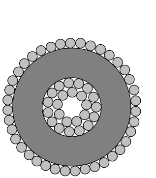
For this purpose, consider the hollow wire configuration illustrated in Figure 1. The inner conductor (made up of a number of windings) carries a strong (and noisy) current which generates a magnetic field ${\bf H}$ within, and outside of, the conductor. Surrounding this inner conductor is a magnetic material which serves to create a large (and noisy) magnetic flux density ${\bf B}$ . The outer conductor carries the return current, and helps confine the magnetic field. An experimental cell can be placed inside the inner conductor for spectroscopic tests. The vector potential inside the cell comes about as a result of the surrounding magnetic flux density. Fluctuations in the current result in fluctuations in the magnetic field, causing fluctuations in the magnetic flux density, producing fluctuations in the vector potential, leading ultimately to a mass shift.

Refer to caption — Figure 1: Hollow wire configuration. The inner conductor (light gray) carries the forward current; the outer conductor (light gray) carries the return current; the magnetic material in between (dark gray) maximizes the magnetic flux density.

5.2 The vector potential

The magnetic field distribution in the quasi-static limit is given in Appendix A. From the resulting magnetic flux density, the vector potential along the axis in the center of the hollow wire configuration is calculated. In the event that the magnetic flux density from the magnetic element of the configuration dominates, the on-axis vector potential is

A_{z}(0)~=~{2N\mu I\over c}\ln{R_{2}\over R_{1}}

(35)

where $N$ is the number of windings, $\mu$ is the permeability of the magnetic element, $I$ is the current, and $R_{2}/R_{1}$ is the ratio of outer to inner radius of the magnetic material.

This approach is conceptually simple, and is capable of generating large vector potentials. Consider an example in which the classical current $I$ is taken to be 1 Amp (which is $2.998\times 10^{9}$ statamps since our formulas are in cgs), and the number of windings $N$ is taken to be unity. The on-axis classical vector potential produced will be 0.1 statvolts (29.98 V) times $\mu$ (assuming the logarithmic term is unity for this exercise). In the case of transformer iron ( $\mu$ = 4000), the resulting vector potential is 400 statvolts (120 kV). For mu-metal ( $\mu$ = 20,000), we obtain 2000 statvolts (600 kV). We conclude that quite high vector potentials can be generated using this approach with only modest experimental requirements.

5.3 Mass shift in terms of current fluctuations

However, the mass shift is sensitive to quantum fluctuations in the vector potential, and not to the expectation value (which corresponds to the classical estimate above). Sizeable fluctuations are difficult to generate, as we see in the following section. In this case, we may write

\delta m~=~{2N^{2}e^{2}\mu^{2}\over mc^{6}}\left(\ln{R_{2}\over R_{1}}\right)^{2}[\langle\hat{I}^{2}\rangle-\langle\hat{I}\rangle^{2}]

(36)

which assumes a mass shift much smaller than the vacuum mass ( $\delta m\ll m$ ).

6 Quantum fluctuations in a lossy driven circuit

So, under what conditions can these fluctuations be maximized? The literature contains numerous papers concerned with the minimization of noise, but in this case we would like to maximize the quantum noise. One approach to the problem is to use a lossy LC-circuit with an amplifier as indicated in Figure 2. This circuit is intended to implement the components that occur in a single mode laser (an oscillator, loss, and gain that saturates), which is known to be very noisy when driven near threshold.

6.1 Master equation

To model intensity fluctuations in the single mode laser (and hence in this kind of circuit), a master equation for the photon probability distribution $p(n,t)$ has been used [23]

{\partial\over\partial t}p(n,t)~=~\alpha[np(n-1,t)-(n+1)p(n,t)]~-~\beta[n^{2}p(n-1,t)-(n+1)^{2}p(n,t)]

~+~\gamma[(n+1)p(n+1,t)-np(n,t)]

(37)

The first term on the RHS accounts for linear gain, where $\alpha$ is a gain parameter. Gain saturation to lowest order is modeled by the second term on the RHS, where $\beta$ is a saturation parameter. The third term accounts for loss, where $\gamma$ is the loss parameter.

In steady state, the probability distribution satisfies

p(n)~=~{\alpha/\gamma\over 1+(\beta/\alpha)n}p(n-1)

(38)

from which an exact solution can be constructed

p(n)~\sim~{(\alpha^{2}/\beta\gamma)^{n}\over\Gamma[(\alpha/\beta)+n+1]}

(39)

6.2 Fluctuations in photon number above threshold

In [23] it is shown that the Stirling approximate can be used to approximate this by a Gaussian, which can be written as

p(n)~\sim~e^{-{1\over 2}(n-\langle n\rangle)^{2}/\Delta n^{2}}

(40)

as long as the average number of quanta $\langle n\rangle$ is much greater than the spread $\Delta n$ . The average $\langle n\rangle$ and spread $\Delta n$ in this model are given by

\langle n\rangle~=~{\alpha-\gamma\over\beta}\ \ \ \ \ \ \ \ \ \Delta n~=~\sqrt{\alpha\over\beta}

(41)

Steady-state fluctuations in this model are maximized when the gain is very nearly matched by the loss ( $\alpha\approx\gamma$ ) for an amplifier with a very low saturation parameter $\beta$ . We can define a difference parameter $\delta$ that is the normalized difference between gain and loss

\delta~=~{\alpha-\gamma\over\alpha}

(42)

In terms of this parameter, the relative fluctuations are

{\Delta n\over\langle n\rangle}~=~{1\over\sqrt{\langle n\rangle\delta}}

(43)

The spread $\Delta n$ for a classical state is simply $\sqrt{\langle n\rangle}$ . The fluctuations here are larger by a factor of $1/\sqrt{\delta}$ due to the diffusion in $n$ associated with the loss and gain in the master equation.

6.3 Current fluctuations above threshold

Fluctuations in the current can be determined from fluctuations in number and phase through a perturbative approach. The expectation value of the current can be related to expectation values of number $\hat{n}$ and phase $\hat{\phi}$ according to

\langle\hat{I}\rangle~=~\sqrt{\hbar\omega_{0}\langle\hat{n}\rangle\over 2L}\cos(\omega_{0}t+\langle\hat{\phi}\rangle)

(44)

We use $L$ for the total inductance of the circuit, and where the characteristic frequency of the circuit $\omega_{0}$ satisfies

\omega_{0}^{2}~=~{1\over LC}

(45)

where $C$ is the capacitance. If the fluctuations are small relative to the average (as depicted in Figure 3), then we can linearize around the sinusoid to obtain

\hat{I}-\langle\hat{I}\rangle~=~{1\over 2}\sqrt{\hbar\omega_{0}\langle\hat{n}\rangle\over 2L}\cos(\omega_{0}t+\langle\hat{\phi}\rangle)\left({\hat{n}-\langle\hat{n}\rangle\over\langle\hat{n}\rangle}\right)\ \ \ \ \ \ \ \ \ \ \ \ \ \ \ \ \ \ \ \ \ \ \ \ \ \ \ \ \ \ \ \ \ \ \ \ \ \

\ \ \ \ \ \ \ \ \ \ \ \ \ \ \ \ \ \ \ -\sqrt{\hbar\omega_{0}\langle\hat{n}\rangle\over 2L}\sin(\omega_{0}t+\langle\hat{\phi}\rangle)(\hat{\phi}-\langle\hat{\phi}\rangle)

(46)

The fluctuations in current are then given by

\langle(\hat{I}-\langle\hat{I}\rangle)^{2}\rangle~=~{1\over 4}\left({\hbar\omega_{0}\langle\hat{n}\rangle\over 2L}\right)\cos^{2}(\omega_{0}t+\langle\hat{\phi}\rangle)\left[{\langle(\hat{n}-\langle\hat{n}\rangle)^{2}\rangle\over\langle\hat{n}\rangle^{2}}\right]\ \ \ \ \ \ \ \ \ \ \ \ \ \ \ \ \ \ \ \ \ \ \ \ \ \ \ \ \

-\left({\hbar\omega_{0}\langle\hat{n}\rangle\over 2L}\right)\cos(\omega_{0}t+\langle\hat{\phi}\rangle)\sin(\omega_{0}t+\langle\hat{\phi}\rangle)\left[{(\hat{n}-\langle\hat{n}\rangle)(\hat{\phi}-\langle\hat{\phi}\rangle)\over\langle\hat{n}\rangle}\right]

+\left({\hbar\omega_{0}\langle\hat{n}\rangle\over 2L}\right)\sin^{2}(\omega_{0}t+\langle\hat{\phi}\rangle)\langle(\hat{\phi}-\langle\hat{\phi}\rangle)^{2}\rangle

(47)

The current fluctuations are due to number fluctuations alone when

\sin(\omega_{0}t+\langle\hat{\phi}\rangle)~=~0

In this case we obtain

\langle(\hat{I}-\langle\hat{I}\rangle)^{2}\rangle~=~{1\over 4}\langle\hat{I}\rangle_{max}^{2}\left[{\langle(\hat{n}-\langle\hat{n}\rangle)^{2}\rangle\over\langle\hat{n}\rangle^{2}}\right]

(48)

6.4 Current fluctuations below threshold

When run below threshold, the excitation of the oscillator is much weaker, so that we can neglect saturation. In this case we obtain a thermal distribution in steady state

p(n)~=~{\alpha\over\gamma}~p(n-1)~=~e^{-\hbar\omega_{0}/k_{B}T_{eff}}~p(n-1)

(49)

where $T_{eff}$ is the effective temperature associated with the amplifier and loss. In the high temperature limit, the current fluctuations are

\langle\hat{I}^{2}\rangle-\langle\hat{I}\rangle^{2}~=~{\hbar\omega_{0}\over L}\left[{1\over e^{\hbar\omega_{0}/k_{B}T_{eff}}-1}+{1\over 2}\right]~\to~{k_{B}T_{eff}\over L}

(50)

6.5 Mass shift estimates

We can use these results to develop estimates for the mass shift. Above threshold, the current fluctuations appear in connection with an oscillating signal, and are limited by how closely the gain matches the loss. Below threshold, only fluctuations occur, and the effective noise temperature is determined once again by how closely the gain matches the loss. In the circuit that we examined here, the gain and loss are variable, but in the steady-state solutions we assumed that they remain fixed. In practice, one would use a more sophisticated arrangement with a very hot resistive element to inject noise (not included in our master equation), and feedback to keep the gain and loss closely matched (not included in our model). Consequently, it makes sense here to characterize the noise in terms of an effective temperature in order to evaluate the magnitude of the mass shift and associated energy shift.

From this discussion, we may write the mass shift in terms of the effective temperature for the below-threshold case as

\delta m~=~{2N^{2}e^{2}\mu^{2}k_{B}T_{eff}\over mc^{6}L}\left(\ln{R_{2}\over R_{1}}\right)^{2}\ \ \ \ \ \ \ ({\rm below~threshold})

(51)

Before continuing, we note that mass shift is maximized when the inductance is minimized, so that no additional inductance should be used. In this case, the total inductance for the circuit is very nearly that of the hollow wire ( $L_{hw}$ ), which is given in Appendix A to be

L_{hw}~=~{2N^{2}\mu l_{z}\over c^{2}}\ln{R_{2}\over R_{1}}

(52)

where $l_{z}$ is the length of the hollow wire. Upon inserting, we obtain for the mass shift

\delta m~=~{e^{2}\mu k_{B}T_{eff}\over mc^{4}l_{z}}\ln{R_{2}\over R_{1}}\ \ \ \ \ \ \ ({\rm below~threshold})

(53)

The associated energy shift evaluates to

\delta mc^{2}~=~5.63\times 10^{-10}~{\rm eV}~\ln{R_{2}\over R_{1}}\left[{10~{\rm cm}\over l_{z}}\right]\left[{\mu\over 20000}\right]\left[{k_{B}T_{eff}\over 1~{\rm eV}}\right]

(54)

Based on this, we would expect that energy shifts in the range of $10^{-9}$ to $10^{-6}$ eV should be possible by maximizing the noise temperature, and by taking advantage of more advanced magnetic materials.

7 Summary and Conclusions

Our effort was stimulated by the recent publication of Widom and Larsen who proposed that a large electron mass shift could be expected to occur near the surface of a metal hydride [13]. These authors were led to this conclusion from a gauge-free formulation of the mass shift. Since the result is so counter to our intuition, we decided to investigate making use of an approach based on the Coulomb gauge. In the end, the key difference is that in the Coulomb gauge one must use the transverse electric field fluctuations for a mass shift estimate instead of fluctuations in the longitudinal field. As a result, the mass shift that we would expect would be orders of magnitude smaller.

As a result of the Widom and Larsen proposal, we were motivated to consider the problem of creating a more significant mass shift than can be obtained thermally, by using nonequilibrium conditions to maximize the fluctuations in the potential vector. To this end, we proposed the use of a hollow wire with a magnetic element driven by a noisy current source; the mass shift in such a configuration is proportional to the current fluctuations of the circuit. To maximize current fluctuations, we considered a lossy LC circuit with an amplifier, which is closely related to the problem of a single mode laser which is known to be extremely noisy near threshold. Fluctuations in the oscillator photon number were modeled using a simple master equation borrowed from laser physics, which has been used to describe the photon distribution in a single mode laser. Above threshold the signal is oscillatory, with small fluctuations which are maximized near threshold. Below threshold, the photon distribution is thermal at a temperature determined by the ratio of the gain to the loss; near threshold, the gain very nearly matches the loss, and the effective temperature can be very high.

To maximize the mass shift, the circuit inductance should be minimized. When the inductance of the hollow wire dominates the circuit inductance, the below-threshold mass shift depends on the permeability, the geometry of the cylinder, and on the noise temperature. It is independent of the number of windings. The mass shift induced in this way is sufficiently large to be observable (we believe that energy shifts in the range of $10^{-9}$ to $10^{-6}$ eV can be produced in a free, or weakly-bound, electron), and it can be greater than the thermal shift observed previously near room temperature. The development of very high noise temperatures in the circuit (in the keV range or higher) will require the use of a more sophisticated circuit than the one analyzed here, since it is difficult to match gain and loss so precisely without feedback.

Note that the mass shift produced in such an experiment occurs under conditions where the classical electric and magnetic fields are zero [in the above threshold case, we are focused on the $\sin(\omega t+\langle\hat{\phi}\rangle)=0$ condition in which the expectation value of the transverse electric field is zero]. It appears as if the electron is exhibiting a response to the vector potential in such an experiment.

Appendix A Classical vector potential estimate

In this appendix we consider the vector potential due to a simple hollow wire configuration as illustrated in Figure 4. The innermost hollow cylinder (between $R_{0}$ and $R_{1}$ ) is a conductor for the forward current, assumed to be made from a nonmagnetic metal such as copper. This conductor is surrounded by a magnetic material (between $R_{1}$ and $R_{2}$ ) such as iron or permalloy. An outer cylindrical conductor is present to carry a return current.

A.1 Magnetic field

If we assume that the current is carried uniformly in the nonmagnetic conductors, and that the system is magneto-quasistatic, then we can estimate the magnetic field using

\oint_{C}{\bf H}\cdot d{\bf l}~=~{4\pi\over c}\int{\bf J}\cdot\hat{\bf n}~d^{2}a

(55)

using circular contours at different radial distances $\rho$ away from the center. We assume that the current in the inner hollow cylinder is $z$ -directed

{\bf J}~=~\hat{\bf i}_{z}J_{0}\ \ \ \ \ \ ({\rm inner~conductor})

(56)

The outer cylinder carries the return current, and is also $z$ -directed

{\bf J}~=~-\hat{\bf i}_{z}J_{1}\ \ \ \ \ \ ({\rm outer~conductor})

(57)

The magnetic field is $\phi$ -directed, and can be estimated simply from Equation (55)

{\bf H}(\rho)~=~\left\{\begin{array}[]{ll}0&0\leq\rho\leq R_{0}\cr\hat{\bf i}_{\phi}\displaystyle{2\pi J_{0}\over\rho c}(\rho^{2}-R_{0}^{2})&R_{0}\leq\rho\leq R_{1}\cr\hat{\bf i}_{\phi}\displaystyle{2\pi J_{0}\over\rho c}(R_{1}^{2}-R_{0}^{2})&R_{1}\leq\rho\leq R_{2}\cr\hat{\bf i}_{\phi}\left[\displaystyle{2\pi J_{0}\over\rho c}(R_{1}^{2}-R_{0}^{2})-\displaystyle{2\pi J_{1}\over\rho c}(\rho^{2}-R_{2}^{2})\right]&R_{2}\leq\rho\leq R_{3}\cr 0&\rho>R_{3}\cr\end{array}\right.

(58)

The magnetic field is zero outside since the return current matches the forward current

J_{0}\pi(R_{1}^{2}-R_{0}^{2})~=~J_{1}\pi(R_{3}^{2}-R_{2}^{2})

(59)

A.2 Vector potential

The vector potential at the $z$ -axis can be found from

\oint_{C^{\prime}}{\bf A}\cdot d{\bf l}~=~\int\mu{\bf H}\cdot d^{2}a

(60)

For this we use a rectangular contour that travels a short distance $\Delta z$ along the $z$ -axis; then radially outward beyond the outer conductor; then backward the same distance in $z$ ; and then radially inward. Since the magnetic field is $\phi$ -directed, no contribution is obtained for the radial legs. Hence, we obtain

[A_{z}(0)-A_{z}(R_{3})]\Delta z~=~\Delta z\int_{R_{0}}^{R_{1}}{2\pi J_{0}\over\rho c}(\rho^{2}-R_{0}^{2})d\rho+\Delta z\int_{R_{1}}^{R_{2}}{2\pi\mu J_{0}\over\rho c}(R_{1}^{2}-R_{0}^{2})d\rho

+\Delta z\int_{R_{2}}^{R_{3}}{2\pi J_{0}\over\rho c}(R_{1}^{2}-R_{0}^{2})-{2\pi J_{1}\over\rho c}(\rho^{2}-R_{2}^{2})d\rho

(61)

Integrating results in

A_{z}(0)~=~\left({2I\over c}\right)\left[\mu\ln{R_{2}\over R_{1}}+{1\over 2}+\ln{R_{3}\over R_{2}}-{R_{0}^{2}\over R_{1}^{2}-R_{0}^{2}}\ln{R_{1}\over R_{0}}+{R_{2}^{2}\over R_{3}^{2}-R_{2}^{2}}\ln{R_{3}\over R_{2}}\right]

(62)

where we have assumed that the vector potential $A_{z}(R_{3})$ is zero outside the outermost conductor.

In the event that the magnetic permeability $\mu$ of the magnetic section is much greater than unity, then the contribution of the magnetic material dominates. In this case, we may write

A_{z}(0)~=~{2\mu I\over c}\ln{R_{2}\over R_{1}}

(63)

A.3 Looped wire

In the event that a high- $\mu$ material is used, then the ratio of vector potential to current can be increased by looping a wire carrying the drive current around the magnetic element, as indicated in Figure 5. The vector potential on axis in this case is

A_{z}(0)~=~{2N\mu I\over c}\ln{R_{2}\over R_{1}}

(64)

where $N$ is the number of windings. The self-inductance of the hollow wire $L_{hw}$ is

L_{hw}~=~{2N^{2}\mu l_{z}\over c^{2}}\ln{R_{2}\over R_{1}}

(65)

where $l_{z}$ is the length of the hollow wire.

References

[1] Feynman R 1948 Phys. Rev. 74 1430
[2] Bethe H A 1947 Phys. Rev. 47 339
[3] Desiderio A M and Johnson W R 1971 Phys. Rev. A 3 1267
[4] Mohr P J 1974 Ann. Phys.(NY) 88 26
[5] Parle A J Aust. J. Phys. 40 1
[6] Eberly J H and Reiss H R 1966 Phys. Rev. 145 1035
[7] Reiss H R 1979 Phys. Rev. A 19 1140
[8] Levinson E J and Boal D H 1985 Phys. Rev. D 31 3280
[9] Barton G 1990 Ann. Phys. NY 200 271
[10] Donoghue J F, Holstein B R, and Robinett R W 1985 Ann. Phys. NY 164 233
[11] Hollberg L and Hall J L 1984 Phys. Rev. Lett. 53 230
[12] Reiss H R 1990 J. Opt. Soc. A 7 574
[13] Widom A and Larsen L 2006 Eur. Phys. J. C 46 107
[14] Lindroth E and Mårtensonn-Pendrill 1989 Phys. Rev. A 39 3794
[15] Panella O, Widom A, Srivastava Y N 1990 Phys. Rev. B 42 9790
[16] Jackson J D 1975 Classical Electrodynamics, John Wiley and Sons, NY
[17] Joulin K, Mulet J-P, Marquier F, Carminati R, and Greffet J J 2004 Surf. Sci. Reports 57 59
[18] Henkel C 2005 Eur. Phys. J. D 35 59
[19] Henkel C, Joulain K, Carminati R, and Greffet J-J 2000 Optics Comm. 186 57
[20] Hauer B, Hempelmann R, Udovic T J, Rush J J, Kockelmann W, Schäfer W, Jansen E, and Richter D 2004 J. Phys.: Condens. Matter 16 5205
[21] Knight P L 1971 J. Phys. A: Gen. Phys., 5 417
[22] Widom A, Srivastava Y N, and Larsen L 2007 LANL Preprint 0709.1222v1
[23] L. Mandel and E. Wolf 1995 Optical coherence and quantum optics, Cambridge University Press, New York. See Chapter 18.
[24] Meltzer D, Davis W, and Mandel L 1970 Appl. Phys. Lett. 17 242