Response of Boolean networks to perturbations
Abstract
We evaluate the probability that a Boolean network returns to an attractor after perturbing nodes. We find that the return probability as function of can display a variety of different behaviours, which yields insights into the state-space structure. In addition to performing computer simulations, we derive analytical results for several types of Boolean networks, in particular for Random Boolean Networks. We also apply our method to networks that have been evolved for robustness to small perturbations, and to a biological example.
pacs
89.75.Hc, 05.45.-a, 89.75.FbI Introduction
Boolean networks (BN) are used to model the dynamics of a wide variety of complex systems, ranging from neural networks [1] and social systems [2] to gene regulation networks [3], sometimes combined with evolutionary processes [4]. BN are composed of interacting nodes with binary states, typically and , coupled among each other. The state of each node evolves according to a function of the states observed in a certain neighbourhood, similar to what is done when using cellular automata [5], but in contrast to cellular automata, BN have no regular lattice structure, and not all nodes are assigned the same update function.
Usually, BN models are studied using deterministic dynamical rules. After a transient time, these networks reach attractors, which are a sequence of periodically repeated states. The number and length of such attractors is an important property investigated in BNs. Of equal importance are the sizes of the basins of attraction of these attractors, which are the sets of states leading to the attractors. Some networks may contain periodic sequences in state space that are not “attractors” in the strict sense, because there are no states outside this sequence that are attracted to it. However, in this paper we do not make this distinction, and we call all sequence periodically repeated sequences of states “attractor”.
Real networks are often influenced by noise, since molecule concentrations may be small (e.g., in biological systems [6]) or behaviour may be unpredictable (e.g., in social systems). For this reason, it is important to investigate how robust the behaviour found under deterministic update rules is when noise is added. Examples for such studies are Ising-like models placed on a network topology [7, 8], BN with a probabilistic rule for choosing the update function at each time step[9], models with stochastic update sequences [10] and small stochastic delays in the update time [11]. These stochastic models can lead to surprising new results. For instance, for stochastic update sequences it could be shown that the number of attractors (now defined as a recurrent set of states) grows like a power law [10, 11] as function of the network size, while it grows superpolynomially for parallel update.
In this paper, we investigate the effect of a perturbation on a BN that is updated in parallel and that is on an attractor. The quantity we evaluate is the probability that the network returns to the same attractor after the perturbation, as a function of the size of the perturbation, i.e., of the number of nodes the states of which are changed. This leads to a curve that is characteristic of the network and is strikingly different for different types of networks.
The outline of this paper is as follows: First, we investigate two types of simple networks, namely networks consisting of independent nodes and networks consisting of a single loop of nodes. The results then help to understand the behaviour of Random Boolean Networks under perturbations, which are studied in Section III dealing with frozen, critical and chaotic networks. In Section IV, we then investigate a few specific networks, which are not random networks, and we find that their characteristic curves are very different from those of random networks, reflecting for instance the higher robustness to perturbations. Finally, we summarize and discuss our findings in Section V.
II Simple networks
II.1 Independent nodes
Let us first consider a system of independent nodes. Then the response of each node to the perturbation is independent of the response of the other nodes. The state of each of the nodes at time is determined by its state at time . There are 4 possibilities to assign to such a node an update function: (i) the state of the node is 0 irrespective of the state at the previous time step; (ii) the state of the node is 1 irrespective of the state at the previous time step; (iii) the state of the node at time is identical to the state at time ; (iv) the state of the node at time is the opposite of the state at time . This means that the node alternates between 0 and 1. The first two update functions are constant functions, the third is the “copy” function, the fourth the “invert” function.
We generate a network by assigning update functions to the nodes. We then initialize the network in a randomly chosen state and wait until it reaches an attractor. In the simple networks considered here, an attractor is reached after one time step. Unless no “invert” function is chosen, the period of the attractor is 2. When a node is perturbed, its response depends on its update function: If the update function is constant, the node returns in the next time step to its previous value. If the update function is “copy”, the node remains in its new state and does not return to its previous state. If the update function is “invert”, the node continues to oscillate between 1 and 0, however with a phase shift of one time step.
When we perturb nodes, the network returns to the attractor only if all perturbed nodes have a constant function, or if all nodes with an “invert” function are perturbed but none with a “copy” function. Let us focus on the case that is large and that each of the four update functions is assigned to one quarter of the nodes. The probability that the network returns to its previous attractor after perturbing nodes is then
| (1) |
which can be approximated by
| (2) |
for . For , the return probability is 0, since it is no longer possible that all perturbed nodes have constant functions. For , it is in principle possible that all nodes with “invert” functions but none with “copy” functions are perturbed, however, the probability that this occurs is so small that we neglect it here.
For general networks, the return probability has to be evaluated by averaging over different initial states, however, in the special case considered here the return probability is the same for each initial state.

The most important result of this subsection is that for small perturbations the return probability is simply given by an exponential dependence
This result will be generally true for small whenever perturbations at different nodes decay independently from each other. For this reason, we will see an exponential decrease in the examples below when is large and is small.
II.2 Simple loops
Now, let us consider a simple loop of nodes.
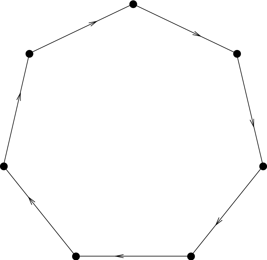
Each node is connected to its predecessor on the loop, and the update function of each node is either “copy” or “invert”. A constant function at one node will freeze the whole loop, in which case for all , and we therefore focus on the more interesting case of no constant function in the loop. A loop with inversions can be mapped bijectively onto one with inversions by replacing two “invert” with two “copy” functions and by inverting the values of all nodes between these two couplings. It is therefore sufficient to distinguish loops with an even or an odd number of inversions, and we call them “even” and “odd” loops respectively. When discussing even loops, we consider loops with only “copy” functions. To odd loops we assign one “invert” function and “copy” functions. An even loop with a prime number of nodes returns to its initial state after time steps. If is not prime, shorter periods exist. Furthermore, if all nodes have the same state, the loop is on a fixed point. An odd loop with a prime number of nodes returns to its initial state after time steps. An odd loop has no fixed points. The shortest attractor has period 2, with alternating 1’s and 0’s.
Figure 3 shows for an even loop with , as obtained from computer simulations.

The return probability is 0 for all odd values of , and it has the same nonzero value for all even larger than 0. This happens for all even loops with being a prime number, as we show in the following. If nodes are perturbed, the loop returns to the same attractor only if the perturbation leads it to another state of this attractor. All states of the same attractor have the same sequence of 0s and 1s, but rotated around the loop by some number of steps. Only by inverting an identical number of 0s and 1s can we stay on the same attractor, and this explains why is nonzero only for even . Now, by fixing the nodes that are to be perturbed and by fixing the number of steps by which the perturbation of these nodes shall rotate the attractor, we uniquely fix the attractor (apart from an inversion of all nodes). This attractor is found by fixing the state of one node to 1 (or 0) and by requiring that the node steps ahead has the same state if the first node is not a perturbed node, and the opposite state if the first node is a perturbed node. Then we determine in the same way the state of the node steps further, and so on, until the state of all nodes is fixed. Since is a prime number, we do not return to the first node before all other nodes have been visited. The probability to be still on the same attractor after perturbing nodes is for even therefore
| (3) |
which is the number of configurations that are rotated by steps under the perturbation, divided by the total number of configurations of the loop. If is not a prime number, there are attractors of different length, and the function depends in a more complicated way on .

For an odd loop with prime , is 1 for and , and has otherwise the value . This result is obtained in a similar way as for even loops: The loop remains on the same attractor after perturbing nodes, if the state generated by the perturbation is among the different states assumed by the loop during the next time steps, but not after steps (where the state of all nodes is simply inverted, which can only be achieved for ). If we fix the nodes to be perturbed and the number of time steps between the unperturbed and the perturbed state, we can uniquely identify the attractor by fixing the state of one node and then stepping around the loop in steps of size , assigning to each node the same state as to the previous node if the previous node is not among the perturbed nodes and if the “invert” function is not between the two nodes. Otherwise, the inverted state is assigned.
II.3 Collections of several loops
If the network consists of several independent loops, the periods of the attractors are the least common multiples of the periods of the loops. Obviously, a collection of loops can remain on the same attractor after a perturbation only if the perturbation produces a state that corresponds to a future state of the loop, but not a state that is not part of the state sequence on this loop. If all loop lengths are different from each other and have no common divisor, every combination of future loop states belongs to the same attractor, and the return probability is identical to the probability that the perturbation generates only such states. Otherwise, if there are two or more loops with periods that have a common divisor, the perturbation must advance all these loops by a multiple of this divisor if the system shall remain on the same attractor. Since the analytical expressions for become complicated and do not provide special insight, we omit them here. We only note that the function depends strongly on the lengths and number of loops, and on the common divisors of their lengths.
III Random Boolean Networks
A random Boolean network (RBN) is constructed by choosing for each node at random nodes from which it receives its input, and an update function that assigns to each of the states of the input nodes an output 1 or 0. The update function of each node is chosen at random among all possible update functions [12, 13]. All nodes are updated in parallel. Depending on the value of and the probabilities assigned to the different update functions, the dynamics of the network is either in the frozen or in the chaotic phase. At the boundary between the two are critical networks. If all update functions are assigned the same probability, RBNs with are in the frozen phase, networks with are critical, and networks with are chaotic. In the following, we consider perturbations of these three types of networks.
III.1 RBNs in the frozen phase
In the frozen phase, all nodes apart from a small number (that remains finite in the limit of infinite system size) assume a constant value after a transient time. If in the stationary state the value of one node is changed, this perturbation propagates during one time step on average to less than one other node. If all nodes that become frozen after some time are removed from the network, there remain the nonfrozen nodes. In the limit , it can be shown that these nonfrozen nodes are connected to simple loops (the “relevant loops”) with trees rooted in the loops [19]. The nodes in the trees are slaved to the dynamics on the loops, and the perturbation of a node on a tree does not induce a change of the attractor. The perturbation of a frozen node can affect a couple of other nodes to which the perturbation may propagate. If these other nodes are also frozen or part of a nonfrozen tree, they will soon return to the behaviour they showed before the perturbation. However, if the perturbation affects a node sitting on a relevant loop, the attractor will usually be changed. If we denote with the probability that the perturbation of one node will affect a node on a relevant loop, we obtain for small . In the limit , the probability must become proportional to , since the number of nodes on relevant loops remains finite in this limit.
From these properties of frozen networks in the limit of large , we can conclude that is close to 1 for , since the probability of perturbing one of the relevant nodes is very small. When becomes of the order of , relevant nodes are perturbed with a considerable probability, and the shape of the function depends on the properties of the relevant loops. The size and number of relevant loops is in general different in different networks. From our discussion in the previous section for collection of independent loops, we conclude that there is no self-averaging of in the limit of large . Also, the probability that the number of relevant nodes is 0 approaches a nonzero constant in the limit , and therefore some networks always have a constant return probability .
Figure 5 shows the result of a computer simulation of three networks in the frozen phase. Half of the nodes were assigned the value and half of the nodes the value . (This combination of values was chosen because networks with are almost always completely frozen. Even for the value , only few networks were not completely frozen.) One can see the inital exponential decay and the broad range of curve shapes when is not small anymore. The behaviour of the curves when approaches depends on the probability that the inversion of the state of all nodes leaves the network in the same basin of attraction. As we can see in this and other figures in this paper, this probability varies widely between networks and is not rarely larger than .

III.2 RBNs in the chaotic phase
In the chaotic phase, initially similar configurations diverge exponentially. Attractors are usually long, and a non-vanishing proportion of all nodes keep changing their state even after long times. Networks with are easiest to understand among the chaotic networks, since the successor of each network state is a randomly chosen other network state [15]. In state space, we have therefore a “network” with one randomly chosen “input” (i.e. successor) for each “node” (i.e., state). In such a network, every perturbation leads the network anywhere in state space, and we therefore expect to be a constant function, with the exception of the value 1 at . The average value of this constant can be determined from what is known for networks: The value of on the plateau is given by the average probability that a randomly chosen state in state space belongs to the same basin of attraction as the randomly chosen initial network state. We define the weight of an attractor as the length of the attractor plus the number of basin states draining into that attractor, normalized by the size of the state space (), so that [16]. We therefore have
| (4) |
| (5) |
leading to
| (6) |
This analytical result applies to the ensemble average of all networks with . In a given network, the value of the plateau usually deviates from 2/3, since always a few large basins dominate the value of , and the values of these basins differ between networks even in the thermodynamic limit.

Now, let us turn to chaotic networks with fixed (smaller than ), for which no such analytical results are known. Figure 6 shows as function of for three networks with and . We see a plateau for , which means that perturbing one or two nodes does not yet necessarily carry the network to a random state, but perturbing several nodes does. The reason for this is that a certain proportion of nodes in chaotic networks with fixed assume a constant value after some time, and perturbing only such nodes may not change the attractor. For larger , it becomes very likely that relevant nodes are changed by a perturbation, and then the situation is similar as in networks, which have no frozen core.
Chaotic networks with fixed value of and large have been shown to share many properties with chaotic networks. From [16], it appears that chaotic networks with have the same set of basin weights as those with , which would mean that the average height of the plateau should be the same for all chaotic networks in the thermodynamic limit. We tested this assumption by simulating smaller networks (of size 20) on the computer for , and . The average of the return probability for a perturbation of size over approximately 10000 networks is , , , and for respectively. These values are impressively close to 2/3 given the small system size. For larger , the value is closer to , because the number of nonfrozen nodes and therefore the size of the (nontrivial part of the) state space increases with increasing . We also simulated systems with larger values of , however, it is very hard to obtain good statistics for larger because the size of the state space and the length of attractors increase exponentially with . From the data we have it appears that the value of the plateau moves closer to 2/3 with increasing . Figure 7 shows the probability distributions of , from which the above-mentioned averages have been obtained. This distribution is very broad and does not appear to become narrower for larger . There is no self-averaging of the plateau value of .
In summary, we find that chaotic networks with large have a return probability that decays rapidly for small and then reaches a plateau, the ensemble average of which lies at .

III.3 Critical RBNs
Critical networks are at the boundary between the frozen and chaotic phase, and neighbouring configurations diverge only algebraically with time. Just as frozen networks, they have a large frozen core. For large , the number of nodes that do not become frozen after some time, is proportional to [19]. Most of them are irrelevant for determining the attractors. When the frozen core is removed from the network, the remaining nodes are connected to relevant components, most of which are simple loops and all of which contain loops, and with trees rooted in these loops. The number of nodes in the relevant components is proportional to for large . The mean number of nodes affected by the perturbation of a single node is for large . The probability that a perturbation of size affects a relevant node is given by the probability that a given node is affected by the perturbation, times the number of relevant nodes, . We therefore obtain
| (7) |
for . This exponential decay can be seen in Figure 8 for small . For , the probability of perturbing a relevant node is not small anymore, and reaches a plateau. A rough estimate of the dependence on of the value of on the plateau is obtained by the following reasoning: The number of attractors increases with roughly as , and the basins of attraction have a size of the order . Using Eq. (4), this gives the estimate on the plateau with some constant . The height of the plateau decreases rapidly with increasing because of the vast number of different attractors of comparable basin size.

Taking these results together, we expect that in large critical networks the function decays from 1 to a value close to 0 when increases from 0 to and then stays on this plateau as increases further. The value of plateau decreases as an exponential function of . However, it is known that the scaling with and of the nonfrozen and relevant nodes becomes clearly visible only in huge networks (of the order ), and smaller networks may show broad distributions in the numbers of these nodes. Figure 8 shows three examples of for critical networks. For such small networks sizes, the critical features of derived for the thermodynamic limit cannot yet be seen.
IV Some specific networks
In the ensemble of all random networks of a not too large size, there are some networks whose characteristic curves are very different from conventional ones, as shown in the next two figures.


The first curve is that of a very robust network, which additionally has the property of returning more easily to the original attractor when the perturbation is larger.
The second curve is that of a network that has no plateau but a very extended decrease of with . A closer inspection of this network reveals that, although its parameter values classify it as critical, there is no frozen core but all nodes are relevant and part of a single complex relevant component. This means that the state space is far from random, and that perturbations of different sizes carry the network to different regions in state space.
Let us compare the first curve to that of networks that have been evolved for robustness to small perturbations [18], shown in Figure 11. These networks have been evolved by modifying the connections and functions and by selecting for a high probability of returning to the same attractor after perturbing one node. Interestingly, although only a large value of has been imposed in the system, is very high for all perturbation sizes. Many networks obtained by the same procedure even show for all .

The network used for producing Figure 12 is the core part of cell cycle regulation network of budding yeast, as represented in [20]. An important property of this network is that it has a prominent fixed point attracting of all network states. The diagram shows the surprising feature that has its minimum at . This means that the main attractor, which is a fixed point, is not very stable under perturbations of one node. Further analysis shows that there are three other fixed points that differ from the main fixed point by the state of only one node. As suggested in [20], the cell is likely to be waiting for a new input when the network is at its fixed point. This might explain why this fixed point is rather sensitive to small perturbations.

V Conclusions
In this paper, we have evaluated the probability that a Boolean network returns to an attractor after perturbing nodes, averaged over different initial states of the network. We found that can display a variety of different shapes, which yields insights into the state-space structure. If the response of the network to the perturbation of several nodes is independent for each perturbed node, decays exponentially with for small . Larger perturbations are of course not independent, and if the perturbation leads the system to a random place in state space, shows a plateau for these perturbation sizes. When the size of the perturbation approaches the total number of nodes, can shown various types of behaviour, including a decrease to zero or an increase to a value larger than the plateau. The reason is that the response to inverting the state of all nodes depends strongly on the network structure. We obtained analytical results for Random Boolean Networks in the limit of large . For critical networks, decreases rapidly to (almost) 0 for large . For chaotic and frozen networks, remains nonzero for large and is not self-averaging, which means that the shape of differs widely between different networks. The ensemble average of the plateau value of for chaotic networks is 2/3 for large . The fact that this plateau value is much higher than in critical networks means that chaotic networks are more robust than critical networks when perturbations affect a nonvanishing proportion of all nodes. The reason for this is that chaotic networks have a much smaller number of attractors than critical networks, and therefore the probability that a perturbation carries the network into the basin of attraction of a different attractor is larger in critical networks than in chaotic networks. Similarly interesting and surprising is the result that a biological network that has been characterized as being very robust is pretty sensitive to perturbations of size , while is much larger for larger perturbations. It remains to be seen if this feature occurs also in other biological networks.
To conclude, characterizing the dynamical stability of networks by a function gives far more information about the state space structure of the network than using a single number, such as the average “sensitivity” of nodes.
VI Acknowledgments
We thank C. Hamer for programming the yeast network and T. Mihaljev for useful discussions.
References
- [1] M. Rosen-Zvi, A. Engel and I. Kanter, Phys. Rev. Lett. 87, 078101 (2001).
- [2] A.A. Moreira, A. Mathur, D. Diermeier and L.A.N. Amaral, PNAS 101, 12085 (2004).
- [3] M.C. Lagomarsino, P. Jona and B. Bassetti, Phys. Rev. Lett. 95, 158701 (2005).
- [4] K.E. Bassler, C. Lee and Y. Lee, Phys. Rev. Lett. 93, 038101 (2004).
- [5] H.J. Herrmann, “Cellular automata” in Nonlinear Phenomena in Complex Systems, ed. A.N. Proto (North-Holland, Amsterdam, 1988), pp. 151-199.
- [6] H.H. McAdams and A. Arkin, Proc. Nat. Acad. Sci. USA 94, 814 (1997).
- [7] J. Indekeu, physics/0310113 (2003).
- [8] A. Aleksiejuk, J.A. Holyst, D. Stauffer, Physica A 310, 260 (2002).
- [9] I. Shmulevich, E.R. Dougherty, and W. Zhang, Proceedings of the IEE 90, 1778 (2002).
- [10] F. Greil and Barbara Drossel, Phys. Rev. Lett. 95, 048701 (2005).
- [11] K. Klemm and S. Bornholdt, Phys. Rev. E 72 (2005) 055101(R).
- [12] S. A. Kauffman,J. Theor. Biol. 22 (1969), p. 437.
- [13] S. A. Kauffman, Nature 224 (1969), p. 177.
- [14] X. Qu, M. Aldana, Leo. P. Kadanoff, Numerical and Theoretical Studies of Noise Effects in the Kauffman Model. Journal of Statistical Physics, 109 (5/6), (December 2002), 967-986.
- [15] Leo Kadanoff and Susan Coppersmith and Maximino Aldana,Boolean Dynamics with Random Couplings, in Perspectives and Problems in Nonlinear Science, A celebratory volume in honor of Lawrence Sirovich, eds. E. Kaplan,J. E. Mardsen and K. R. Sreenivasan (2003), Springer, New York.
- [16] P. Krawitz and I. Shmulevich,Basin Entropy in Boolean Network Ensembles, 2007 cond-mat/0702114
- [17] B. Derrida, J. Phys. 48, 971 (1988).
- [18] A. Szejka, B. Drossel, Eur. Phys. J. B 56 373-380 (2007)
- [19] V. Kaufman, T. Mihaljev, B. Drossel, Phys. Rev. E 72, 046124 (2005)
- [20] F. Li, T. Long, Y. Lu, Q. Ouyang, C. Tang, PNAS 101 4781-4786 (2004)