Establishment of the Coulomb law in the layer phase of a pure U(1) lattice gauge theory
Abstract
In this article we examine the Layer phase of the five dimensional, anisotropic, Abelian gauge model. Our results are to be compared with the ones of the 4D U(1) gauge model in an attempt to verify that four dimensional physics governs the four dimensional layers. The main results are i) From the analysis of Wilson loops we verified the behavior, in the layered phase, for the potential between heavy charges. The renormalized fine structure constant in the layer phase is found to be equal to that of 4D Coulomb phase,=. ii) Based on the helicity modulus analysis we show that the layers are in the Coulomb phase while the transverse bulk space is in the confining phase. We also calculated the renormalized coupling and found results compatible with those obtained from the Coulomb potential. Finally we calculated the potential in the 5D Coulomb phase and found behavior for the static potential. From the study of the helicity modulus we have a possible estimate for the five dimensional renormalized fine structure constant in the region of the critical value of the bare gauge coupling .
Physics Department, National Technical University,15780 Zografou Campus, Athens, Greece
1 Introduction
The idea that we live on a hypersurface embedded in a higher dimensional space has attracted the interest of particle physicists and cosmologists in connection with the hierarchy and the cosmological constant problems. These ideas are motivated by string- and M-theory that are formulated in multidimensional spaces. One version is to consider the extra dimensions flat, compactified to a large scale varying from the Planck scale to a few TeV depending on the number of extra dimensions [1, 2]. An alternative concept is the so called brane world scenario [3], where all of the particles are localized on a three-dimensional submanifold (brane), embedded in a multidimensional manifold (bulk), while gravitons are free to propagate in the bulk. This model in five dimensions, implies a non-factorizable space time geometry of the form around the brane, assuming a negative five-dimensional cosmological constant . The four-dimensional particles are expected to be gravitationally trapped on the brane. Indeed gravitons and scalars for the second RS model [3] have a localized solution on the brane, plus a continuum spectrum . Gravitons, scalars and fermions also exhibit a normalizable zero mode localized on the brane if we assume a non trivial scalar background in the bulk, such as a kink topological defect toward the extra dimension [4]. The most difficult task is the massless non-abelian gauge field localization on the brane, as any acceptable mechanism must preserve the charge universality [5]. A localization mechanism that may be triggered by the extra dimensional gravity is proposed by the authors of refs [6, 7, 8]. It is based on the idea of the construction of a gauge field model which exhibits a non-confinement phase on the brane and a confinement phase on the bulk, that is to say, a higgs mechanism driven by the coupling with the gravity. Thus gauge fields, and more generally fermions and bosons with gauge charge, cannot escape into the bulk unless we give them energy greater than the mass gap , which emerges from the nonperturbative confining dynamics of the gauge model in the bulk. In a previous work [9] we have studied the 4+1 dimensional pure Abelian Gauge model on the lattice with two anisotropic couplings, independent from each other and the coordinates, focusing our attention to the study of the phase diagram and the order of the phase transitions. With this model we wanted to explore the possibility of a gauge field localization scheme based on the observation that the anisotropy of the couplings produces a new phase, the layer phase, which mimics the Coulomb behavior in four dimensions but confines along the remaining one. This model is known since the mid-eighties when Fu and Nielsen proposed it as a new way to achieve dimensional reduction [10]. It is defined on a D-dimensional space containing d-dimensional subspaces. If the couplings in the d-dimensional subspaces are identical () and the remaining coupling coefficients are also to be taken identical (), then for a certain range of parameters (typically and )** * This result comes from the mean field analysis of the theory. this new phase emerges. The confinement along the directions and the resulting detachment of the d-dimensional layers leads to the following physical picture. Charged particles in the layer phase will mainly run only along the layers since if they attempt to leave the layers in which they belong they will be driven back by a linear potential, analogous to the one responsible for quark confinement. Also gauge particles will follow the layers since there is no massless particle (photon) moving across the layers. We must note here however that a stable layer phase exists only if and for the U(1) model. For we cannot have a layer phase since lattice gauge theory in less than four dimensions exhibits confinement for all finite values of the coupling constant, rendering the 3-dimensional subspaces of the model incapable of realizing a Coulomb phase . Also, due to the asymmetric role of and in the action, there is no layer phase with their roles reversed.
Many numerical investigations of the model have been made using Monte-Carlo techniques, verifying the structure of the phase diagram and the properties of the different phases [11, 12, 13]. In one of them [11] the presence of fermions in the model was investigated. The analysis, both analytical (mean field approximation) and numerical (Monte Carlo simulations) revealed that the qualitative characteristics of the phase diagram remained unchanged, even though a slight restriction of the layer phase was observed in favor of the Coulomb one. In [12] the authors analyzed the structure of a U(1) model when the coupling in the fifth dimension depends on the coordinates exponentially, like in the RS model [3]. In ref[13] the 5D anisotropic abelian Higgs model was analyzed and the existence of a layer Higgs phase was established. Finally, we would like to mention the main results in [9] for the phase diagram of the pure U(1) anisotropic gauge model: i) a weak first order phase transition between the 5D strong phase and the layer phase with the characteristics of 4D U(1) and ii) strong indications for a second order transition between the layer phase and 5D Coulomb phase. In a preliminary study of the six dimensional U(1) model we have found that the characteristics of the strong-layer phase transition remained the same but at the same time the transition between the layer and the 6D Coulomb phase turned into a strong first order one.
For the case of the anisotropic non-Abelian SU(2) gauge model the above picture changes [14]. Now the critical dimension for the formation of the layers is D=6 giving as a minimal dimension for the layers d=5. But, as it is shown in ref [15] a Layer Higgs phase in the non-abelian 5D model exists if one includes a scalar field in the adjoint representation.
In the present work we will focus our attention on the study of the long range interactions of charged particles on the layers, at an attempt to further justify our previous assumption [9] that the layers incorporate all the features that emerge in ordinary U(1) gauge theory in 4-dimensions. To this end a very significant step is the establishment of the Coulomb law and for that we follow the usual approach: Measurements of Wilson loops (on the layers and for the 4-dimensional model), subsequent extraction of the potential and finally, estimates for the string tension () and the renormalized charge or fine structure constant () are obtained. An equally important byproduct of the above analysis is determination of the role of layer-layer interactions and their consequences (if any) for the physical picture in the layers.
Our work is organized as follows. In section 2 we present the four dimensional model along with the various analysis techniques used throughout this paper. In section 3 we present the layer phase results and a comparison with their 4D counterparts and finally, in section 4, we concentrate in the 5D Coulomb phase in order to show the clear distinction (both qualitative and quantitative) from the layer one as well as an attempt to explore the very nature of what should be a five-dimensional Coulomb law.
2 The 4-dimensional case
2.1 Wilson loops and the static potential
One of the observables used in lattice gauge theories with great physical significance, is the Wilson loop defined as the gauge invariant quantity consisting of an ordered product of link variables along a contour C. If we denote by such a link variable then the Wilson operator is defined as
| (2.1) |
and its expectation value on a rectangular loop C is:
| (2.2) |
where and are the (dimensionless) spatial and
temporal extention of the contour C. The symbol
denotes the expectation value with respect to the 4d gauge action:
From the asymptotic behavior of the above quantity we can (in principle) derive the potential between two static charges using numerical methods through the formula
| (2.3) |
There are also R-independent self energy contributions to that one has to take into account (see next section).
2.2 Helicity Modulus and the renormalized coupling
A very usefull quantity for the characterization of phases in lattice gauge theories
is the helicity modulus (), first introduced in this context
by P.de Forcrand and M.Vettorazzo [16]. It characterizes the responce of a
system to an external flux and has the behavior of an order parameter.
It is zero in a confining phase and nonzero in a coulombic one [16, 17].
The helicity modulus is defined as:
| (2.4) |
were is the external flux and the flux free energy given by:
| (2.5) |
with the partition function of the system due to the presence of the external flux.
is the sum over the stack of plaquettes, of a given orientation (e.g )
in which the extra flux is imposed (), and
is its complement, consisting of all the plaquettes that remained unchanged.
An observation that will subsequently play an important role is that the partition
function of equation (2.5) and hence the flux free energy is clearly
periodic . So, the extra flux we impose on the system is defined only
.
If we, take for example: then, with a suitable change in variables we can spread the extra flux uniformly to all the plaquettes in the () plane. The partition function now becomes
| (2.6) |
and from equation (2.4) we get for the h.m:
| (2.7) |
with the sum extending to all planes parallel to the given orientation.
Now, consider for the moment the classical limit () for the action of equation (2.6) where all the fluctuations are suppressed. In this limit the flux is distributed equally over all the plaquettes of each plane and does not change as we cross parallel planes. If we expand the classical action in powers of the flux [16], since in the thermodynamic limit is always a small quantity, we find:
where V is the lattice volume, .
The above expression for the free energy F holds all the way up to the phase transition, where fluctuations are present, if one only replaces the bare coupling by a renormalized coupling: (for details see [16, 17]).
Upon replacing the above expression becomes:
| (2.8) |
The above equation does not show any periodicity in . To remedy this situation we have to consider all configurations whose flux is a multiple (k) of .
| (2.9) |
Now we can define implicitly from the equation:
| (2.10) |
As equations (2.9) and (2.10) show, the renormalized coupling equals the helicity modulus up to exponentially small corrections [16].
2.3 Measurements
Our Monte Carlo calculations for the case of four-dimensional QED are restricted to volumes , and . For all lattice sizes, the work of Jersak et al [18] has been closely followed. We used a 5-hit Metropolis algorithm supplemented by an overrelaxation method. About sweeps were used for thermalization and more than 2 x measurements, 10 sweeps apart from each other, for the determination of mean values. For the case of all planar rectangular Wilson loops with R=1,…,6 and T=1,…8 were calculated while for the rest we used loops in an effort to minimize finite size effects.
In general, one has to extract the potential from the logarithms of the expectation values of Wilson loops for large T.
| (2.11) |
This however requires a large enough volume to deal with the many issues that emerge in lattice calculations. Finite size effects are a constant “threat” to the validity of the results and in addition finite T effects must also be taken into account in the extraction of the potential. This means that significant deviations from a linear dependence on T should be investigated. To this end, a third term in the above equation is introduced
| (2.12) |
with C actually being a function of R.
The form of the “correction” term is an open question but we choose as it is the simplest (and most obvious) choice. The potential V(R) has been calculated using both linear (eq. (2.11)) and non-linear (eq. (2.12)) dependence of the logarithms on T, at a variable number of points dependent on the volume under consideration, giving comparable results within errors. The resulting values were fitted to a superposition of linear + Coulomb potentials :
| (2.13) |
and
| (2.14) |
with the lattice Fourier transform of a massless bosonic propagator [18, 19] which respects not only the momentum cut-off but also accounts for the periodicity of the lattice.
| (2.15) |
All measurements focused on the Coulomb phase starting from values near the critical point and extending to larger values of . In Table 1 we present the results for several volumes using both the continuum (eq. (2.13)) and the lattice Coulomb potential (eq. (2.14)) obtained from the non-linear fitting (eq. (2.12)). The notation we use is indicative. With we imply the use of continuum Coulomb potential () and with the use of lattice Coulomb potential (eq. (2.15)). A few remarks are now in order. First of all, the estimates of using the two different types of potential, show a systematic deviation of the order of 0.010 - 0.020 which was also found to be true by Jersak et al [18]. Second, it is evident from Table 1 that the values of show a quick convergence to the infinite volume limit as their deference, between the biggest volumes that we used ( and ) is well within errors. The string tension starts at relatively large values due to finite size effects for the smaller system under study, only to reach a final value of 0.003 as the volume increases. This result is slightly bigger than the one found by Jersak et al. It appears that the reason for this systematic overestimation of has its origin at the insertion of the extra term () of equation (2.12). This extra term inserts an ”effective” string tension that adds up to the measurement, but this was anticipated. In ref [19] it was found that the static charge potential obtained from Wilson loops, acquires a confining contribution for finite volume. This term has exactly the same form as the term () that we have added by hand and consequently we have enhanced an already present confining contribution to the potential. One could in general monitor the contribution of this extra term and subtract it in order to remedy the presented inconsistency between the values of the string tension () as they are obtained through the use of equations (2.11) and (2.12) (Tables 1 & 2). Unfortunately, knowledge of the precise functional dependence of C from R is required, a topic that proves to be not an easy task. So, in order to extend our measurements for the renormalized charge to smaller volumes we have enhanced the signal for the string tension. This however does not affect the obtained values of , a fact most apparent in the subsequent analysis. In Table 2 we present our results for a linear fit (equation (2.11)) and L=16 for both types of potential (ontinuum oulomb and attice oulomb). Comparing with Table 1, for L=16, one can see that by reaching a big enough volume the extra term does not play any substantial role. Insofar as is concerned, linear and non-linear fits give exactly the same results (within errors) (Figure.1). The string tension is found smaller and compatible with zero within the statistical errors. The linear fit gives us a more convincing signal for the vanishing of the string tension with values comparable with the ones found by Jersak et al [18].
| L=16 | ||||
| 1.015 | 0.1860(20) | 0.0033(5) | 0.1693( 9) | 0.0027(3) |
| 1.020 | 0.1765(16) | 0.0035(4) | 0.1605( 9) | 0.0030(3) |
| 1.030 | 0.1631(13) | 0.0036(3) | 0.1484(11) | 0.0030(3) |
| 1.050 | 0.1472(12) | 0.0033(3) | 0.1339(11) | 0.0027(3) |
| L=14 | ||||
| 1.015 | 0.1883(34) | 0.0039(10) | 0.1692(12) | 0.0024(3) |
| 1.025 | 0.1716(26) | 0.0040(10) | 0.1540(11) | 0.0027(3) |
| 1.030 | 0.1632(23) | 0.0034(10) | 0.1474(14) | 0.0023(4) |
| 1.040 | 0.1577(29) | 0.0035(10) | 0.1414(12) | 0.0027(3) |
| 1.050 | 0.1472(21) | 0.0045(15) | 0.1329(14) | 0.0020(4) |
| L=12 | ||||
| 1.013 | 0.1975(2) | 0.0060(10) | 0.1765(12) | 0.0041(3) |
| 1.015 | 0.1906(2) | 0.0060(10) | 0.1708(14) | 0.0040(3) |
| 1.025 | 0.1730(2) | 0.0055(20) | 0.1552(12) | 0.0040(2) |
| 1.050 | 0.1537(2) | 0.0055(10) | 0.1366(10) | 0.0038(2) |
| 1.060 | 0.1466(2) | 0.0055(10) | 0.1307(10) | 0.0034(2) |
| 1.100 | 0.1338(2) | 0.0050(10) | 0.1182(10) | 0.0035(2) |
| 1.200 | 0.1087(2) | 0.0050(10) | 0.0968(10) | 0.0026(2) |
| L=16 | ||||
|---|---|---|---|---|
| 1.015 | 0.1868(30) | 0.0010(7) | 0.1698(23) | 0.0020(6) |
| 1.020 | 0.1771(26) | 0.0005(6) | 0.1610(23) | 0.0010(6) |
| 1.030 | 0.1638(22) | 0.0003(5) | 0.1488(20) | 0.0010(5) |
| 1.050 | 0.1476(20) | 0.0003(4) | 0.1342(18) | 0.0008(5) |

In 1982 Luck [20] using the close analogy between the 2-dimensional XY model and 4-dimensional compact QED arrived by means of a weak-coupling expansion, at the following form for the behavior of the renormalized fine structure constant
| (2.16) |
with and . The analysis lead him to the conclusion that the square of the renormalized charge takes a universal value =1.90 0.10 at the deconfinement point.
By making use of equation (2.16) and the most accurate (to our knowledge) value for the critical in four dimensions ( [21]) we present in Table 3 our results for and , were the last row (L=16) refers to the results of the linear fit and the L=10 entry actually amounts to a lattice volume. Our values are in very good agreement with those found in ref[18] and those predicted through theoretical calculations [20]. The systematic error in the analysis due to the presence of turns out to be insignificant.
| L | |||||
|---|---|---|---|---|---|
| 10 | 0.230(25) | 0.208(24) | 0.31( 8) | 0.33(10) | 1.05 |
| 12 | 0.209( 7) | 0.200( 4) | 0.38( 5) | 0.34( 3) | 0.80 |
| 14 | 0.211(23) | 0.190(10) | 0.44(20) | 0.45(13) | 0.75 |
| 16 | 0.211(16) | 0.190( 9) | 0.42(16) | 0.43(10) | 0.20 |
| 16 | 0.211(23) | 0.192(21) | 0.43(10) | 0.42(15) | 0.10 |
A pleasing fact is that both types of potential manage to describe equally well our data, giving identical results (within errors) and thus providing us with a signal for the existence of a massless photon in the Coulomb phase. The only noticeable difference between the two sets comes from the appearance of a systematic volume dependence for , with evidence that better accuracy is provided by the lattice potential, as it better takes into account the system volume. Finally, the inclusion of the extra term () proved quite efficient, since it allowed us to obtain the required information even at smaller volumes.
3 The 5-dimensional anisotropic model, layer phase
3.1 The model
In this section we consider the five dimensional anisotropic U(1) lattice gauge model with two couplings and :
| (3.17) |
where
are the plaquettes defined on the 4-d subspace ( = 1,2,3,4) and on the plane containing the transverse fifth direction () respectively . †† † By and we denote the two different lattice spacings: one referring to the 4-dimensional subspaces and the other to the transverse fifth direction. The link variables are defined as:
and in terms of them the plaquette variables can be written as
with the definitions
Before we proceed we would like to define the helicity modulus for this model. The anisotropy of the couplings and the resulting enrichment of the phase diagram introduces the necessity for two kinds of h.m. One probing the response of the system to an external flux through the spatial planes () and one for the transverse planes ().
| (3.18) |
| (3.19) |
with the sum of equation (3.3) extending on all the plaquettes on the transverse plane.
The phase diagram of this model includes three distinct phases (Fig.2). For large values of the couplings (, ) the model lies in a oulomb phase on a 5D space. Now, with fixed, as decreases the system will eventually develop a behavior according to which the force in four dimensions will be Coulomb-like while in the fifth direction the system will exhibit confinement. This is the new ayer phase. For small values of both and the force is confining in all five directions and the coresponding phase is the trong phase.
The Wilson loops and the helicity moduli are expected to exhibit different behavior as one crosses the phase boundaries. In the trong (confinement) phase all Wilson loops obey the area law while at the same time the helicity modulus is zero throughout the appropriate range of parameters, both signals for confinement. In the 5D oulomb phase the opposite picture emerges. Wilson loops obey the perimeter law with the helicity modulus being nonzero and scaling with the lattice length as and increase. A five dimensional Coulomb-type force is present. Finally, the ayer phase consists of a mixture of both aforementioned phases. The Wilson loops constrained in the 4d subspaces ( with ) obey the perimeter law while at the same time those that contain the fifth direction (, ) show an area law behavior. The helicity modulus shows also two different behaviors. The space h.m ()) has a nonzero value in the layer phase while the transverse h.m () is constrained to a zero value as one would expect from a confining force (Figure 8).
3.2 Measurements
The calculations of this section are dedicated entirely to the layer phase for the range of parameters =0.2 and . In order to illustrate the qualitative and quantitative agreement between the layer phase of the 5 dimensional model and the corresponding 4d systems we focused on and volumes, which in the context of the layer phase translates to ten and twelve layers of volume and each‡‡ ‡ In the notation that will be used from now on 4D will signify the four dimensional model while 4d the four dimensional subspaces (layers) of the five dimensional system. . Every layer is (to a very large extent) decorrelated [13] from the others and every quantity measured on it a random variable with a given distribution. So, it really does not matter which layer we choose to observe, since each one of them will demonstrate exactly the same behavior. If we treat the system as a whole this would only amount to an increase in statistics. In order to probe the physics in the layers all planar rectangular Wilson loops with R=1,…,5 and T=1,…,8 and R=1,…,6 and T=1,…,6 depending on the case under study were constructed from link variables living only on the 4-dimensional subspaces () §§ § Although finite size effects forced us to disregard all borderline sizes. while at the same time independent runs were made to the corresponding 4-dimensional models (, V=) for a straightforward comparison. Following the same steps as in the previous section we investigated the long range correlations, in terms of the dimensionless parameter , in these two different systems.
3.2.1 The 16 case
We use equation (2.12) in order to extract the potential from the mean values of the Wilson loops. All points with T=1,2 were excluded from the fits and even T=3 for (Fig.3) [18]. We were able to determine the potential V(R) only at 4 points R=1,…,4 for each value of (because of the “noise” introduced by finite size effects) and compare these values with the ones from the 4-dimensional model.


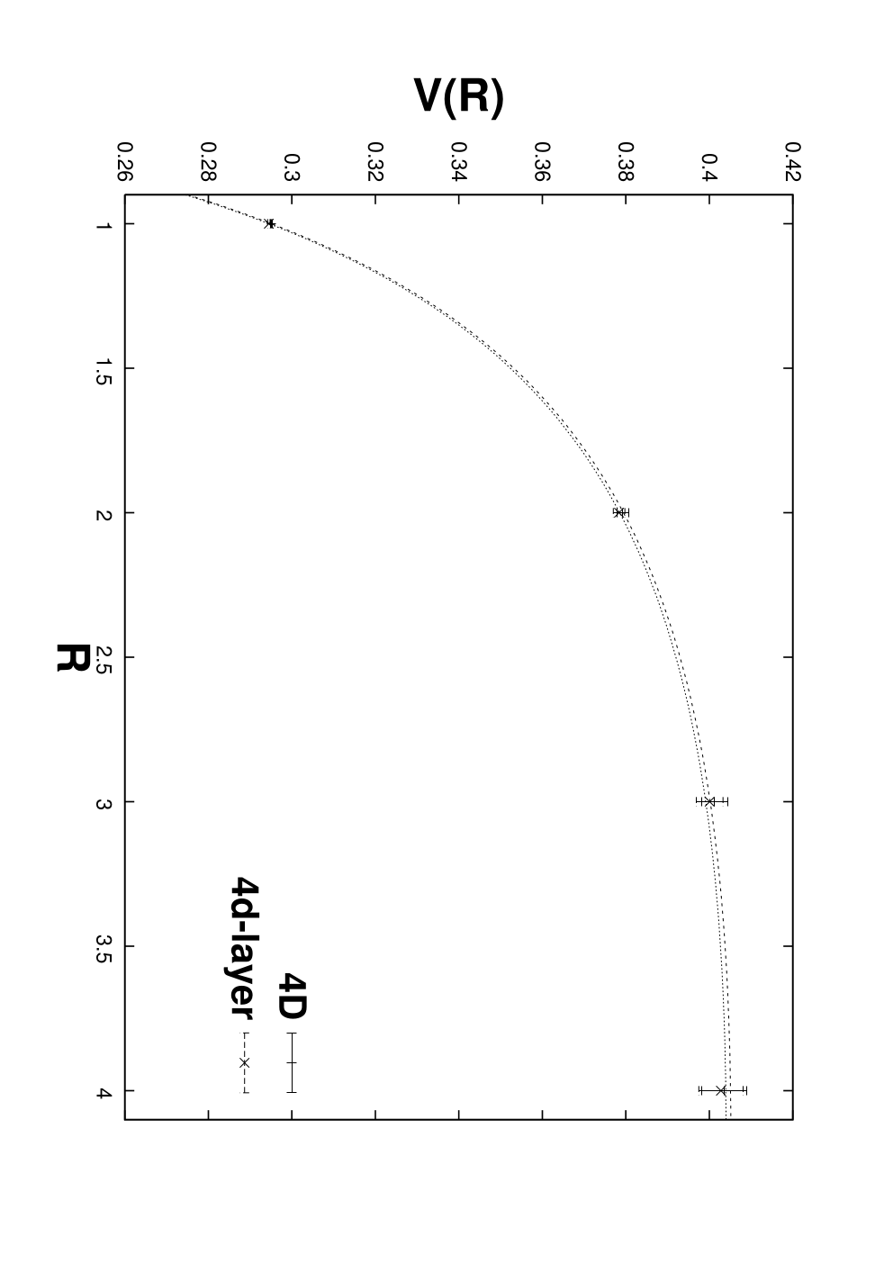
The obtained values were fitted to a superposition of a linear + oulomb potentials for both forms of the latter (ontinuum and attice). The behavior describes well the data (Fig.4(a)) and gives results compatible with the ones obtained from the 4D model (Fig.4(b)). This serves as a first signal for the presence of a four dimensional Coulomb law in the layer phase. The second, and most important, is the fact that equally good results are provided by means of the four dimensional lattice propagator (eq. (2.15)), a quantity that describes the long range interactions in four dimensional lattices. The success in the description of the data comes as strong evidence of the four dimensional nature of the layers.
So, it seems that both signals, the form of the potential in the layers and the success of the massless bosonic propagator in the description of the data, which by itself could be considered as evidence of the presence of a massless boson acting as mediator to the forces in the layer, point to the existence of a 4d gauge particle in the layer phase with all the characteristics of an “ordinary” photon. In Tables 4 and 5 we present the results for and for the two models, and . The similarity between the two sets of measurements is very encouraging. The two systems reveal exactly the same behavior (as it is demonstrated by the two measured quantities) regardless of the form chosen for the Coulomb potential.
| 1.015 | 0.1910(88) | 0.0110(35) | 0.1907(80) | 0.0110(33) |
| 1.030 | 0.1677(78) | 0.0107(30) | 0.1683(75) | 0.0108(30) |
| 1.050 | 0.1517(55) | 0.0098(32) | 0.1522(68) | 0.0100(27) |
| 1.070 | 0.1411(64) | 0.0093(26) | 0.1412(67) | 0.0093(26) |
| 1.080 | 0.1367(62) | 0.0090(25) | 0.1370(63) | 0.0090(25) |
| 1.090 | 0.1330(62) | 0.0087(24) | 0.1332(20) | 0.0088(25) |
| 1.100 | 0.1295(63) | 0.0085(23) | 0.1298(30) | 0.0083(19) |
| 1.200 | 0.1101(40) | 0.0079(23) | 0.1093(23) | 0.0070(20) |
| 1.300 | 0.0900(100) | 0.0065(35) | 0.0932(17) | 0.0060(18) |
| 1.400 | 0.0830(40) | 0.0054(22) | 0.0822(40) | 0.0049(16) |
| 1.015 | 0.1747(80) | 0.0097(34) | 0.1753(73) | 0.0097(34) |
| 1.030 | 0.1541(70) | 0.0096(29) | 0.1546(70) | 0.0096(28) |
| 1.050 | 0.1394(64) | 0.0089(27) | 0.1397(63) | 0.0090(27) |
| 1.070 | 0.1296(61) | 0.0083(25) | 0.1322(69) | 0.0083(25) |
| 1.080 | 0.1256(59) | 0.0080(24) | 0.1258(59) | 0.0081(25) |
| 1.090 | 0.1221(59) | 0.0078(24) | 0.1223(54) | 0.0079(24) |
| 1.100 | 0.1189(56) | 0.0075(23) | 0.1192(50) | 0.0075(22) |
| 1.200 | 0.1065(60) | 0.0068(24) | 0.0981(48) | 0.0062(20) |
| 1.300 | 0.0792(96) | 0.0057(20) | 0.0855(44) | 0.0054(17) |
| 1.400 | 0.0763(38) | 0.0048(16) | 0.0754(39) | 0.0043(16) |
We repeat the whole analysis for the linear case using equation (2.11) since our “correction” term only affects the T direction and, as is evident from our 4-dimensional study, the value T=16 proves to be sufficient. The agreement between the relevant sets of measurements (Tables 6 & 7) is extremely good (indistinguishable within the errors) as one can also see in Figures 5(a) & 5(b).
| 1.015 | 0.1967(133) | 0.0097(51) | 0.1974(136) | 0.0098(52) |
| 1.030 | 0.1734(120) | 0.0095(46) | 0.1741(115) | 0.0095(45) |
| 1.050 | 0.1567(112) | 0.0088(43) | 0.1574(112) | 0.0089(43) |
| 1.070 | 0.1459(107) | 0.0083(41) | 0.1462(106) | 0.0083(41) |
| 1.080 | 0.1413(101) | 0.0080(39) | 0.1418(103) | 0.0081(40) |
| 1.090 | 0.1372(101) | 0.0079(35) | 0.1378(100) | 0.0078(33) |
| 1.100 | 0.1341( 97) | 0.0076(37) | 0.1344( 95) | 0.0077(35) |
| 1.200 | 0.1115( 90) | 0.0075(35) | 0.1105( 83) | 0.0063(32) |
| 1.300 | 0.0961( 70) | 0.0054(28) | 0.0965( 75 ) | 0.0055(27) |
| 1.400 | 0.0860( 66) | 0.0048(25) | 0.0864( 65) | 0.0050(25) |
| 1.015 | 0.1806(122) | 0.0083(50) | 0.1812(124) | 0.0080(50) |
| 1.030 | 0.1592(110) | 0.0082(45) | 0.1597(111) | 0.0080(50) |
| 1.050 | 0.1438(103) | 0.0076(43) | 0.1444(103) | 0.0076(40) |
| 1.070 | 0.1339( 98) | 0.0072(40) | 0.1341( 98) | 0.0073(40) |
| 1.080 | 0.1296( 93) | 0.0069(38) | 0.1301( 94) | 0.0070(40) |
| 1.090 | 0.1259( 91) | 0.0067(36) | 0.1264( 92) | 0.0068(40) |
| 1.100 | 0.1230( 89) | 0.0065(37) | 0.1234( 85) | 0.0064(35) |
| 1.200 | 0.1024( 86) | 0.0076(36) | 0.1013( 76) | 0.0055(33) |
| 1.300 | 0.0883( 66) | 0.0047(27) | 0.0884( 69) | 0.0051(30) |
| 1.400 | 0.0790( 60) | 0.0042(25) | 0.0793( 60) | 0.0040(20) |


3.2.2 The case
The analysis presented above is now repeated for a larger system, at an attempt to further strengthen our results. For the extraction of the potential from Wilson loops only equation (2.12) has been used. Although we had to restrict ourselves to smaller Wilson loops, due to the smaller extend of the lattice in the ”time” direction, and utilize a much larger statistics for the 5D model the aforementioned picture does not change.


We present our results for the potential V(R) in Figure 6 ((a) and (b)). The continuum Coulomb potential () is used to fit the data from R=1 to R=5 with extremely good accuracy, is always in the range 0.8-1.1.
| 1.015 | 0.1898(32) | 0.0080(20) | 0.1906(16) | 0.0075(15) |
| 1.025 | 0.1778(40) | 0.0070(10) | 0.1730(15) | 0.0060(10) |
| 1.050 | 0.1541(33) | 0.0060(10) | 0.1537(12) | 0.0060(10) |
| 1.100 | 0.1333(26) | 0.0050( 5) | 0.1338(13) | 0.0050(10) |
| 1.015 | 0.1735(10) | 0.0060(20) | 0.1708(14) | 0.0040(2) |
| 1.025 | 0.1588(10) | 0.0052(20) | 0.1552(12) | 0.0040(2) |
| 1.050 | 0.1386( 6) | 0.0045(14) | 0.1366(10) | 0.0038(2) |
| 1.100 | 0.1184( 5) | 0.0037(11) | 0.1182(10) | 0.0035(2) |


As it is evident from Figure 6 and Tables 8 & 9, where we compare results for the two different systems: in the Coulomb phase and in the layer phase, for the same , the presented consistency cannot pass unnoticed. It is not only the qualitative characteristics of the layer phase that point to the 4-dimensional nature of the forces governing the layers but also the quantitative agreement with results from the pure 4D model. We found that all results from this section for the effective fine structure constant fall on the same region of values making them almost indistinguishable as Figure 7 shows.
3.2.3 The renormalized fine structure constant, a summary of results
We find with the help of equation (2.16) and Tables 4 and 5, fitting using that:
=0.230(30) =0.32(10) =0.210(30) ()
=0.230(25) =0.31( 8) =0.208(24) = 0.33(10) ()
And for the linear fits, from Tables 6 and 7 we have:
=0.235(49) =0.32(16) =0.216(45) ()
=0.238(52) =0.31(16) =0.219(48) ()
Finally from Tables 8 and 9 we have:
=0.201(14) =0.51(22) =0.198(08) ()
=0.209(07) =0.38(05) =0.200(04) ()
using the continuum () and lattice Coulomb () potential respectively. ¶¶ ¶ Although the values of come very close to the value predicted at large R from the picture of the rough string [22], this should be ascribed to the small four dimensional volume..
We can conclude that the layer-layer interactions are negligible and as a result the interaction between two charges on a layer is a long range Coulomb interaction with a massless carrier the photon.
3.2.4 Results from the helicity modulus
The main effort, as far as the h.m is concerned, was focused on volumes and for the four and five dimensional systems respectively. We supplement the 5D results with data from our previous work [9].

As the Figure 8 and Table 10 reveal, the 4d subspaces (layers) of our model realize the above transition the exact same way as a 4D system realizes the passage from a confining phase to the Coulomb phase. The transverse h.m () remains zero throughout the transition, indicating confinement through the fifth direction while at the same time the space h.m (), measured on the layers, obtains the same values as the corresponding quantity of the four dimensional model.
| 1.015 | 0.4941(22) | 0.1611(7) | 0.4908(8) | 0.1622(4) |
| 1.025 | 0.5455(15) | 0.1460(5) | 0.5462(5) | 0.1458(3) |
| 1.050 | 0.6216(14) | 0.1281(4) | 0.6196(4) | 0.1285(2) |
| 1.100 | 0.7134( 9) | 0.1116(4) | 0.6196(5) | 0.1116(2) |
| 1.200 | 0.8526( 6) | 0.0934(3) | 0.8520(3) | 0.0935(1) |
Using the values we found from the helicity modulus (Table 10) and adopting the
behavior of equation (2.16) for we have :
=0.198(4) =0.28(2) ()
=0.201(2) =0.276(8) ()
These results are to be added to the ones of the previous subsection and the excellent agreement for the renormalized fine structrure constant with the lattice Coulomb results must be noticed.
4 The Coulomb phase
Looking in the 5D (,) phase diagram (Figure 2) there is a separate phase for big values of and which we mention as a Coulomb 5D phase. In order to characterize this phase we calculate the potential V(R) between two heavy charges using the same techniques as in sections 2 and 3. If we follow the diagonal line = there is a first order phase transition between the 5D strong phase and the 5D Coulomb phase for approximately ==0.74 as we show in Figure 9.
For this part of our study we go deep in the 5D Coulomb phase following the diagonal line of = in the phase diagram for the biggest volume under study (). By taking the gauge couplings equal, the previous anisotropy of the model is now lost. As a consequence most equations used in the previous sections recive an almost natural generalization to five dimensions.


Due to the passage from a 4-dimensional world (3+1) to a higher dimensional one
(n + 3 + 1 ) the form of the Coulomb potential changes. The
behavior no longer holds. The extra dimensions add powers to the denominator resulting to a
power law. We remind that:
using for the calculation spherical co-ordinates:
Keeping all this in mind a natural generalization of equation (2.13) would be, for the
case of a 5-dimensional Coulomb potential:
| (4.20) |

| /d.o.f | |||
|---|---|---|---|
| 1.100 | 0.0330(9) | 0.00033(24) | 0.67 |
| 1.200 | 0.0293(8) | 0.00033(25) | 0.74 |
| 1.300 | 0.0264(6) | 0.00028(18) | 0.66 |
Equation (4.1) describes well our data (Figure 10 and Table 11) while at the same time additional endorsement comes from the fact that all attempts to use the 4-dimensional potentials for the description of the data were fruitless, with a ranging from 7 to 20, thus excluding any connection with a 4D law. Another point worth mentioning is that even if we subtract the confining term () from equation (4.1) we still get acceptable results ( 1-1.2) with the resulting change in the values of beeing within errors.
With the form of potential established to we continue with the generalization of equation (2.15) to five dimensions.
| (4.21) |
| (4.22) |
| /d.o.f | |||
|---|---|---|---|
| 1.100 | 0.0298( 4) | 0.0005(3) | 1.68 |
| 1.200 | 0.0265( 6) | 0.0004(2) | 1.90 |
| 1.300 | 0.0239(10) | 0.0004(2) | 1.80 |
The above values are not as good, in terms of the , as the ones obtained from the continuum Coulomb potential. They show a systematic deviation of order 10%-12% from our previous results but that was also the case for the measurements of section 3. Nevertheless they constitute a second estimate for the effective fine structure constant in five dimensions.
Finally we go on and measure the helicity modulus for this phase to acquire our final estimate for . Due to the homogeneity of the model in the line the choice of the plane in which the extra flux is imposed is not restricted, since all the planes are now equivalent. Every possible choice will lead us to the same result (a fact verified by our measurements). So, we continue with what we shall generally call helicity modulus in 5D () measured on the ( planes).
| (4.23) |
Lets pause here for a moment to consider the classical limit of the above equation. With
all fluctuations suppressed we have (following subsection 2.2) :
Again, with the replacement and use of equation (2.10) we have for the helicity modulus:
| (4.24) |
Hence the h.m scales with the lattice length and as one approaches the infinite volume limit the signal obtained from this quantity is infinitely enhanced. Although the argument presented above is based mainly on the classical approach, this is indeed the case and the helicity modulus applied for the five dimensional system behaves exactly as equation (4.5) predicts. So, in order to extract the value of , the appropriate rescaling is needed. To that end, all measurements in this section concerning the h.m are the product of the simple rescaling that equation (4.5) suggests . In Table 13 one can find the verification of all this where the estimates from the two lattice volumes ( and ) are identical, within the error bars.
| 0.800 | 0.5017(4) | 0.0505(2) | 0.5014(4) | 0.0506(2) |
| 0.900 | 0.6312(4) | 0.0402(2) | 0.6306(5) | 0.0402(3) |
| 1.000 | 0.7460(3) | 0.0339(2) | 0.7458(3) | 0.0340(2) |
| 1.100 | 0.8547(3) | 0.0297(1) | 0.8539(7) | 0.0297(1) |
| 1.200 | 0.9611(2) | 0.0264(1) | 0.9610(2) | 0.0264(1) |
| 1.300 | 1.0653(3) | 0.0238(1) | 1.0657(2) | 0.0238(1) |
| 1.400 | 1.1693(2) | 0.0217(1) | 1.1694(2) | 0.0217(1) |
As Table 13 shows the agreement between the values of as they are obtained from the five dimensional helicity modulus and the corresponding lattice Coulomb potential (Table 12) is almost perfect. The measurements of the helicity modulus are extended near the critical point in order to sketch the behavior of the effective renormalized charge as we approach the transition. We observe that there is no volume dependence as the difference between the results from the two lattice volumes is within the statistical error.
5 Conclusions
Throughout this whole investigation we observed no discrepancy between the two systems at any point: The 4D pure U(1) gauge model in the Coulomb phase and the anisotropic 5D U(1) model in the layer phase exhibit exactly the same behavior. From the values and the form of the potential, to the estimates for the renormalized coupling and the string tension and finally to the values of and . All signals point to the four dimensional nature of the long range interactions in the layers and the presence of a massless particle, the photon, albeit the need for larger volumes. The obtained agreement respponds, indirectly, on another subtile matter, which is the role of the layer-layer interactions in the physical picture. It seems, to the extend that we can observe, that there is no evidence of any significant influence that could lead to an essential alteration from the known four dimensional laws. To clarify this point we would like to add a few remarks regarding the nature of the gauge particle. Fu and Nielsen, in a followup work [10], have thoroughly examined the properties of this gauge particle. Their analysis suggested, from a strong coupling expansion point of view, that to lowest-order approximation the photon propagator is identical with the one in the isotropic 4-dimensional U(1) gauge field model. But, upon corrections the propagator received contributions from the layer-layer coupling (). Taking into account the contributions of all graphs consisting of plaquettes connecting neighboring layers (by means of an effective action) they have managed to show that to order
for links in the same layer. ∥∥ ∥ Ordinary propagator means a propagator for which =0 so that all layers are isolated from each other. But, for the range of our measurements, corrections of this order of magnitude are put into shadow by our error estimates. It is beyond our measuring capabilities to examine the possible reprecautions of such a term and the differentiations that it could lead. On the optimistic side though, for the whole range of the parameters that we used for our analysis this “correction” ranges from 0.999967 (starting point) to 0.999976 (end point). So we strongly doubt that any meaningfull diversion from the four dimensional law can be found.
A second point that deserves attention is the use of the helicity modulus for the extraction of the renormalized coupling (). The obtained information from the use of this quantity is in very good agreement with the results obtained from the traditional method of determination of using the Wilson loops, with one advantage: it is much cheaper, from a computer power(/time) point of view, to use the helicity modulus than to resort to Wilson loops. The required information comes directly from a single measurement, without any intermediate steps, thus reducing drastically the complexity of the method, compared to the usual approach. To that end (and) for the characterization of the various phases of our model we find the helicity modulus a much better tool than Wilson loops.
Finally, in the 5D Coulomb phase we found that the values of the effective (=) are smaller than the values of effective = as our results indicate and also that the effective is slightly bigger than the bare coupling == , where = the dimensionless 5D bare U(1) gauge coupling **** ** here is the 5D lattice spacing and the ultraviolet cutoff.. The values of that we used for the determination of the 5D Coulomb potential are far away from the phase transition. In order for someone to be able to compare results between 4D and 5D an extrapolation up to the critical point is neccesary. To that end, we calculated the helicity moduli for two different volumes (Table 13) and fitted the results using equation (2.16) under the assumption that there is no drastic change in the behavior of as we go to five dimensions and consequently, that the equation remains still valid for the particular case under study. We used the critical value of as a free parameter and found: (i) that there is no volume dependence and (ii) the renormalized fine structure constant takes the value of =0.218(48), a value near to the one in four dimensions and =0.49(37). Unfortunately the quality of the fit was not pleasing (, hence the large errors) but it did manage to reproduce the value of the critical in the correct region ().
Because the 5D QED is not a pertubativelly renormalizable field theory and the gauge coupling has Mass dimensions () , powers of the cutoff appear in the calculations of loops corrections (see [2] and references therein) to the vertex and self energy graphs. In the lattice calculations the cutoff does not appear explicitly but only implicitly through the volume dependence of Monte Carlo results. So, in the presence of matter fields, we expect a strong volume dependence for the effective renormalized charge in the extrapolation to the critical and to the infinite volume, different from what we found in the present paper for the pure U(1). This study is outside the scope of this work but we believe that it deserves further investigation.
6 Acknowledgements
We acknowledge support from the EPEAEK programme “Pythagoras II” co-funded by the European Union (75%) and the Hellenic State (25%). We are very greatfull to P.de Forcrand for a series of very usefull conversations regarding the helicity modulus and its applications and to G.Koutsoumbas, K.Anagnostopoulos and P.Dimopoulos for their help and support, for reading and discusing this manuscript.
References
- [1]
I.Antoniadis Phys.Lett.:377-384,1990;
I.Antoniadis, K. Benakli Phys.Lett.:69-78,1994 [hep-th/9310151];
Nima Arkani-Hamed,S.Dimopoulos,G.R.Dvali Phys.Rev.:086004,1999
[hep-ph/9807344];
Nima Arkani-Hamed,S.Dimopoulos,G.R.Dvali Phys.Lett.:263-272,1998 [hep-ph/9803315];
C. P. Bachas :023,1998 [hep-ph/9807415] - [2] K.R.Dienes, E.Dudas, T.Gherghetta Nucl.Phys.:47-108,1999 [hep-ph/9806292]; Keith R. Dienes , Emilian Dudas , Tony Gherghetta Phys.Lett.:55-65,1998 [hep-ph/9803466].
- [3]
L.Randall , R.Sundrum Phys.Rev.Lett.:4690-4693,1999. [hep-th/9906064];
L.Randall , R.Sundrum Phys.Rev.Lett.:3370-3373,1999. [hep-ph/9905221];
B.Bajc, G.Gabadadze Phys.Lett.:282-291,2000. [hep-th/9912232];
I.Oda Phys.Lett.:113-121,2000 [hep-th/0006203];
A.Perez-Lorenzana . J.Phys.Conf.Ser.:224-269,2005. [hep-ph/0503177] - [4] A. Kehagias, K. Tamvakis Phys.Lett.:38-46,2001 [hep-th/0010112]; V.A. Rubakov, M.E. Shaposhnikov Phys.Lett.:136-138,1983; V.A. Rubakov, M.E. Shaposhnikov Phys.Lett.:139,1983.; H. Davoudiasl,J.L.Hewett,T.G.Rizzo Phys.Lett.:43-49,2000 [hep-ph/9911262]; T.Gherghetta,A.Pomarol Nucl.Phys.:141-162,2000 [hep-ph/0003129]; A.Pomarol Phys.Lett.B486:-157,2000 [hep-ph/9911294]
- [5]
V.A. Rubakov Phys.Usp.:871-893 [hep-ph/0104152];
S.L. Dubovsky, V.A. Rubakov Int.J.Mod.Phys.:4331-4350,2001 [hep-th/0105243] - [6] K. Farakos, P. Pasipoularides Phys.Lett.:224-232,2005 [hep-th/0504014]
- [7] K. Farakos, P. Pasipoularides Phys.Rev.:084012,2006 [hep-th/0602200]
- [8] K. Farakos, P. Pasipoularides Phys.Rev.:024018,2007 [hep-th/0610010]
- [9] P. Dimopoulos , K. Farakos, S. Vrentzos Phys.Rev.:094506,2006 [hep-lat/0607033]
- [10]
Y.K. Fu , Holger Bech Nielsen Nucl.Phys.:167,1984.;
Y.K. Fu , Holger Bech Nielsen Nucl.Phys.:127,1985. - [11] A.Hulsebos,C.P.Korthals-Altes,S.Nicolis Nucl.Phys.:437-451,1995 [hep-th/9406003]
- [12] P.Dimopoulos, K.Farakos, A.Kehagias and G.Koutsoumbas Nucl.Phys.:237-252,2001 [hep-th/0007079]
- [13]
P.Dimopoulos,K.Farakos Phys.Rev.:045005,2004 [hep-ph/0404288];
P.Dimopoulos,K.Farakos,S.Nicolis Eur.Phycs.J.,87,2002 [hep-lat/0105014];
P.Dimopoulos,K.Farakos,C.P.Korthals-Altes,G.Koutsoumbas,S.Nicolis
JHEP :005,2001 [hep-lat/0012028] - [14]
D.Berman, E.Rabinovici Phys.Lett.:292,1985
Y.K. Fu, Liang-Xin Huang and Da-Xin Zhang Phys.Lett.:65-70,1994 - [15] P.Dimopoulos, K.Farakos and G.Koutsoumbas, Phys.Rev.:074505,2002 [hep-lat/0111047]
- [16]
Michele Vettorazzo, Philippe de Forcrand Nucl.Phys.Proc.Suppl.:739-741,2004
[hep-lat/0311007];
Michele Vettorazzo, Philippe de Forcrand Nucl.Phys.:85-118,2004 [hep-lat/0311006];
Michele Vettorazzo, Philippe de Forcrand Phys.Lett.:82-90,2004 [hep-lat/0409135] - [17] J.L.Cardy Nucl.Phys.:369-387,1980
- [18]
J. Jersak, T. Neuhaus, P.M. Zerwas Nucl.Phys.:299,1985.;
J. Jersak, T. Neuhaus, P.M. Zerwas Phys.Lett.:103,1983. - [19] G. Cella, U.M.Heller, V.K.Mitrjushkin and A.Vicere Phys.Rev.:3896-3902,1997 [hep-lat/9704012]
- [20]
J.M. Luck Nucl.Phys.:111,1982
- [21] G. Arnold, B.Bunk, T.Lippert and K.Schilling Nucl.Phys.Proc.Suppl.:864-866,2003 [hep-lat/0210010]
- [22]
M.Luscher,K.Symanzik and P.Weisz Nucl.Phys. (1980) 365;
M.Luscher, Nucl.Phys. (1981) 317.