Coarse graining of master equations with fast and slow states
Abstract
We propose a general method for simplifying master equations by eliminating from the description rapidly evolving states. The physical recipe we impose is the suppression of these states and a renormalization of the rates of all the surviving states. In some cases, this decimation procedure can be analytically carried out and is consistent with other analytical approaches, such as in the problem of the random walk in a double-well potential. We discuss the application of our method to nontrivial examples: diffusion in a lattice with defects and a model of an enzymatic reaction outside the steady state regime.
I Introduction
Many problems of relevance in physics, chemistry and biology are appropriately described as systems of interacting, discrete entities which evolve according to stochastic rules. These entities may be not all equal, for example they may be molecules of different chemical species. When a) there is spatial homogeneity and other continuous degrees of freedom are irrelevant for the description, and b) the Markovian property holds, such systems are well described by master equations,
| (1) |
Here denotes the state of the system, is the probability of being in state at time , and is the transition rate from state to state . For instance in multi-species chemical systems, is a vector , the component being the number of molecules of the -th specie.
The description of chemical and biological processes in terms of master equations is usually rather accurate. However, it can have rather severe problems, even in the numerical treatment, if the number of states is large and overall if many degrees of freedom are involved. When the number of particles is large enough, a possibility is to describe the dynamics in terms of concentrations: there are several methods to move from a master equation to a partial differential equation, like the Van Kampen system size expansion [1]. The most common result of such a procedure is a Fokker-Plank equation.
On the other hand there are systems which are fundamentally discrete and, therefore, the continuous approximation may give answers which are quite different from that of the discrete case, like enzymatic reactions which are often studied in the limit where one has many substrate molecules but very few enzymes [2]. Other notable examples are genetic systems working with low molecules copy numbers [3, 4] and ecological systems close to the extinct absorbing state [5].
A common features of many of these problems which can be used to simplify the description is the presence of many relevant timescales. Sometimes the timescale of the interactions is fast, but due to the many degrees of freedom the timescale of the global dynamics is much slower. This is the case of protein folding: while the elementary time scale of vibration of covalent bonds is , the folding time for a protein may be of order of seconds. Another problematic situation is when the degrees of freedom are not so many, but the interactions are of diverse nature, resulting in entries in the transition matrix of very different orders of magnitude. An example of the latter case comes from many cell regulatory systems: proteins in a cell can interact chemically, again on molecular timescales, and via transcription regulation, on timescales of seconds or even minutes. In all these situations one says that the system has a multiscale character [6].
The necessity of treating the “slow dynamics” in terms of effective equations is both practical (even modern supercomputers are not able to simulate all the relevant scales involved in certain difficult problems) and conceptual: effective equations are able to catch some general features and to evidence key controls and basic ingredients which can remain hidden in the detailed description. The study of multiscale problems has a long history in science: perhaps the first example is the study, due to Newton, of the precession of the equinoxes, which was basically a special version of the averaging method in mechanics [7]. In fluid dynamics an example of the multiscale procedure is the derivation of an effective Fick equation for the large scale and long time behavior starting from the transport equation [8]: the diffusion tensor depends, often in a non intuitive way, on the velocity field. Finally, in quantum mechanics, since the nuclei are much heavier than the electrons, one can simplify the treatment “splitting” the electronic and nuclear degrees of freedom, like in the Born-Oppenheimer approximation [9], or in its modern generalization due to Car and Parrinello [10].
Multiscale systems described by master equations can be difficult to deal with. Gillespie’s stochastic simulation algorithm [11], which is an exact and well established method for numerical simulations of master equations, is not very efficient to simulate multiscale systems. The reason is that Gillespie algorithm treats fast and slow dynamics on equal footing, while if one is interested in the slow dynamics it is usually not necessary (and computationally demanding) to exactly integrate the fast dynamics. In recent years, several authors introduced modifications and approximations of the Gillespie algorithm that allow to improve its efficiency when applied to multiscale problems. Many approaches have been developed like the quasi-steady state approximation [12, 13], fast variables elimination methods [14, 15], finite state projection techniques [16, 17], or continuous approximations of fast variables [18, 19].
The method developed in this paper follows a different idea. We want to study master equation containing states with fast and slow dynamics (evolving with different characteristic times). Our approach is to write down an effective master equation describing the evolution of the slow states only. The physical recipe we are going to impose is that, looking at the system on a slow timescale, the time spent on the fast states can be neglected. These states are thus eliminated from the description and this brings to new effective transitions among the slow states. Clearly this approximation gives better results when the separation of timescales between fast and slow states becomes large. Our procedure, by reducing the number of states, may allow for a large gain in simulation time. However, our main goal is to obtain in a systematic way a simple description of a system obeying a master equation on a slow timescale. Indeed, we will show that in some cases our method does not correspond only to a numerical recipe, but allows for analytical predictions.
The plan of the paper is the following. In Section II we introduce our method. Section III is devoted to the one dimensional examples: a random walk in a double-well potential and a random walk in a lattice with defects. Section IV we apply our method to a common model of enzymatic reaction and show how it can predict its behavior far from the steady state regime. Conclusions and perspectives are in section V.
II The method
Let us introduce the intuitive idea of the method with a schematic example. We consider the motion of a Brownian particle in a potential having minima, like the one sketched in Fig. 1.

When the temperature is not too large the probability distribution function of the particle is concentrated only around the the minima and . Therefore, instead of the complete Fokker-Planck description, it is sensible to study the system in terms of a Master equation with states: we say that the system is in the state when is close to . Moreover, we consider the case in which the barriers between states , and , have the same height , being smaller than the height of the barrier between states and . In this case, one has two very different typical times: the transition time between states , and , and the transition time between and , . If one is interested to properties on times much longer than , it is quite natural to devise a model of the system with only two states, say which includes and and which includes and . This simple example suggests how the study of a system on a slower timescale may lead to a reduction in the number of states one has to consider.
Consider now a generic master equation
| (2) |
The standard way to simulate the above equation would be of course the Gillespie algorithm [11], which is exact and does not imply a choice of a timestep. On the other hand, we would like to select a (slow) timescale, so let us discuss what happens if we integrate naively the equation, for example discretizing the time via the Euler algorithm:
| (3) |
In this case, the application of the Euler algorithm corresponds to approximate the master equation with a Markov chain, defined by the Markov transition matrix
| (4) |
where we introduced for convenience of notation the total out-rate of state ,
| (5) |
When integrating Eq.(2), should be chosen to be small compared to the timescales of the system dynamics. However, notice that Eq.(2) and (3) share the same stationary condition independently on . This means that they have the same stationary state for any , even though they can have in principle quite different dynamics when increases. A natural question is what happens when becomes large. The problem one encounters is that the diagonal element of the matrix (4) can become negative. This starts happening when
| (6) |
On the other hand, when , the Markov chain and the original master equation are closely related. Not only they share the same stationary state, but one can easily write a relation between their eigenvalues, which are in a one to one correspondence. We can write the Markov matrix :
| (7) |
where is the identity and is the matrix having as non-diagonals elements the transition rates and on the diagonal minus the total out-rates. This implies that, calling and the eigenvalues of the matrices and , one has
| (8) |
Another way of seeing it is that is the first-order expansion of the evolution operator of the master equation . This implies the error one makes on the eigenvalues is order and should be negligible for the slower modes when is not too large.
II.1 Decimation procedure
Eq. (6) suggests a strategy to identify “fast states” on a given timescale. The idea is that, every time a generic state is reached, the average time spent in it is . As a consequence, if we choose the parameter representing the smaller timescale we aim to describe, then all states having should not enter into the description. In order to eliminate them, the physical recipe we impose is simply that the time spent on these states is zero. In this way, the states disappear from the dynamics and the transition rates from a generic state to a generic state are modified according to:
| (9) |
This procedure corresponds to adding to the rate the process of going to with the proper rate and then instantaneously going to with the proper probability. A graphical example of the application of the method is shown in Fig. (2).

II.2 Commutativity and adiabatic approximations
A natural question at this point is whether the order of elimination of the “fast states” matters for the resulting dynamics . In presence of two fast “linked” states, say and , such that , and or , the result of decimation could be different, in principle, depending on the order of elimination of the “fast states”, i.e. before and them or viceversa.
To show that our procedure commutes in general and clarify the connection with adiabatic approximations, let us rearrange the vector into two vectors where is a vector containing the probabilities of the slow states and contains the probabilities of the fast states. We rewrite the master equation as:
| (10) |
The adiabatic approximation corresponds to set , that is
| (11) |
We can safely assume since otherwise the probabilities of the slow states would be zero at equilibrium. So we can solve the above equation for and substitute it into the equation for :
| (12) |
Notice that Eq. (12) preserves normalization since
| (13) |
in other words, within the adiabatic approximation there is no probability flow between fast and slow states. Eq.(12) may thus be considered a bona fide reduced master equation for the slow degrees of freedom, with the transition rates being renormalized due to the effect of the fast states. Notice that, at variance with fast variables elimination methods [14], the probabilities are not marginalized probabilities, meaning that we didn’t average over fast states. The probabilities of fast states can be eventually reconstructed as a function of time after solving the equations for the slow states.
To clarify the relationship between Eq. (12) and our method, notice that condition (11) is a linear set of equations for the fast degrees of freedom. Let us consider the solution obtained by the substitution method: we start eliminating a particular fast state by computing its probability from the -th equation:
| (14) |
It should be clear at this point that, by substituting the above expression in the evolution equation of a fast state, the original rule of Eq. (9) is retrieved; the same procedure can be iterated to solve the probabilities of all the fast states and substitute it into the remaining equations. The conclusion is that our method is equivalent to solve the condition (11) using the substitution method. But since the solution of that condition is unique, the resulting master equation will be Eq.(12), independently on the order of elimination of the fast variables.
III One dimensional examples
Now we apply our decimation procedure to some one dimensional random processes. The first example is the well known problem of the double well; in this case the decimation procedure can be carried out analytically and predict the correct transition rate between the two minima. The second example is a one dimensional random walk with defect.
III.1 Double well potential
Let us consider the problem of a random walk in a double-well potential. This example is paradigmatic both in physics and in kinetic chemistry, in the latter case the one-dimensional axis represents the reaction coordinate and one is interested the rate of jumping from one minimum to the another, i.e. of the reaction to occur. Again, we assume that this axis is subdivided in discrete states . We can introduce the potential , which determines the following transition probabilities:
| (15) |

being the usual Boltzmann factor. Notice that the above transition rates ensure that at equilibrium the probability of being in state is proportional to . We do not restrict ourself to a particular choice of the potential, we just assume that the potential has two minima which we denote with and , as sketched in Fig.(3). As usual, we are free to choose a value of and eliminate all the states whose inverse out-rate is smaller than :
| (16) |
By increasing , the two minima are the last two surviving states since in a minumum both the exponentials in Eq.(16) have negative arguments. This means that with a proper choice of the time scale we can end up with a two state Markov chain and calculate the transition rate between the two minima.
By alling the number of states between and , the transition rate writes:
| (17) |
In the denominator we indicate with the notation the total out-rate of state to remember that this out-rate changes when a neighboring state is eliminated. This means that the product of out-rates has to be evaluated by eliminating the states one after the other. To evaluate the expression (17), we make use of the following equality, which is demonstrated in the Appendix:
| (18) |
with the convention that products of less than one terms are always equal to one, . Substituting (15) and (18) into (17) one obtains:
| (19) | |||
where in the last step we assumed that the potential does not change much between adjacent states. The last expression is basically the well known result for the transition rate in a double well potential in a continuous system described by a Fokker-Planck [20].
III.2 Random walk with defects
Considered now a random walker in a one dimensional geometry with periodic boundary conditions; the number of its possible states is fixed to . The transition rate between two adjacent states is except for a fraction of the states (the “defects”), having . The defects are placed at random at the beginning and kept the same in all the simulations (quenched disorder). In solid state physics the master equation of this system corresponds to the Schrödinger equation (at imaginary time and with disorder) in the limit of tight binding approximation [21].
Clearly one has for the normal states and for the defects. This means that the defects are the fast states and we will test what happens when eliminating them from the description. For comparison, we will see also the differences with the ideal case without defects, that is for all the states.
It is easy to analytically calculate the eigenvalues in the case without defects [21]:
| (20) |
Notice that all the eigenfunction are non-localized, which in solid state physics corresponds to a conductive system. On the contrary, in the case with defects (for any positive value of ) the eigenfunctions are localized, i.e. one has a transition from a metal to an insulator [22].

In Fig.(4) we show the eigenvalues of the master equation in the three cases: random walk without defects, with defects and after decimation. Being the master equation linear, the eigenvalues spectrum contain all the informations about the dynamics. The spectrum shows an interesting property: the most negative eigenvalues are much larger in modulus and correspond to fast decaying eigenfunctions concentrated on the defects. It is clear from the figure that the effect of our algorithm is to eliminate these eigenvalues (and the corresponding eigenfunctions).
It is clear in the figure that the 100 eigenvalues smaller in modulus, corresponding to the slower dynamics of the system, are very similar in the model with defects and the decimated one. A further check comes from the correlation functions. We performed the simulations starting from a slow state and plotted in Fig. 5 the probability of being in the state as a function of time in the three cases we considered. After an initial time, the correlation functions for the decimated model and the model with defects are very close to each other.

IV Enzymatic reactions
In this section we apply our method to a model of enzymatic reactions. Enzymatic reactions are widely studied in kinetic chemistry and many methods have been derived to predict the steady-state kinetics in cases in which the reaction is close to an equilibrium, or at least in a non equilibrium steady state [23]. To exemplify the relevance of our method in this case, we will consider in the following the simplest model of an enzymatic reaction:
| (21) |
where as usual denotes the enzyme, the substrate and the reaction product. This correspond to the following master equation:
| (22) | |||
where we called the number of free (non binded) substrate molecules, the number of free enzymes molecules, and the total number of enzyme molecules. We also introduced, as usual, the total out-rate of a general state:
| (23) |
The quantity of interest is usually the production rate, that is the velocity of the rightmost reaction as a function of the concentration of enzymes and substrate. It is easy to estimate it in the quasi-equilibrium approximation, that is when , meaning that the leftmost part of the reaction can be considered at equilibrium. Another thing one can assume is steady state dynamics: the calculation is simple even if the complex is not at equilibrium but the concentration of the complex does not vary much with time, . The steady state approximation is known to hold very well when the concentration of enzymes is much smaller than that of substrate.
In this case the reaction velocity follows the Michaelis-Menten formula:
| (24) |
where . In order to apply our method, we start from Eq. (23). The expression for the out-rates suggests two limiting cases in which there is separation of scales between fast and slow states. The first case is . In this case, states having have a much greater out-rate than those with and can be coarse-grained. Physically it corresponds to the situation in which the complex is efficiently processed, so that its concentration is always very close to zero. In this case the application of our method yields:
| (25) |
Notice that we wrote the rate in term of (the total number of substrate molecules) and not since with the coarse graining we grouped together states with bounded and free substrates as long as the total number is the same. Notice also that this rate correctly corresponds to the Michaelis Menten formula, eq. (24) taken in the limit . The new information provided by our method is that in this limit the linear dependence on the number of substrates is valid also beyond the steady state approximation, that is when the enzymes concentration becomes large.
The second limiting case is . In this case, all states having and are fast. This means that, for a fixed , the slow state is characterized by . When we retrieve again the steady state result:
| (26) |
The above expression, again, is consistent with the Michaelis-Menteen equation, this time in the limit when the reaction rate does not depend anymore on the substrate concentration. On the other hand, when one has:
| (27) |
This last case is radically different with the steady state prediction: we have a linear dependence on the number of substrate molecules while Michaelis-Menteen formula predicts a rate which is independent on . The physical reason is that this is a case in which the complex never reaches a steady state: on a fast timescale, order the free substrate is completely converted into the complex . Then it is depleted on much slower times, and the depletion speed is limited by the lower between the enzyme and the substrate concentration.

In Fig. (6) we plot simulations of the reaction (21) in four different situations. The top left figure corresponds to the situations in which and (numerical values of the parameters are in the figure caption), together with the prediction of Eq. (25), while on the top-right we show and with the prediction of Eq. (26). These two are the cases in which steady state approaches are known to work and our approach simply corresponds to the limiting cases of Michaelis-Menten formula. On the bottom figures we show the same cases, but with . Notice that the left one correspond to the top/left one, rescaled with the higher number of enzymes; in particular, it is still described by Eq. (25). On the other hand, the bottom-right is even qualitatively different from the corresponding top figure. Eq.(27) correctly describes the behavior, while Michaelis Menten formula would predict the rate to be independent of .
In order to study also the fluctuations of the process, we simulated both the full master equation and the simplified processes defined by Eq. (25), (26) and (27). Then we compare in Fig. (7) the variance of the number of product molecules as a function of time. The result of the simulations is that the fluctuations are almost indistinguishable in the reduced processes: the intuitive reason is that most of the fluctuations are related to the slow states and thus unaffected by the coarse graining procedure.
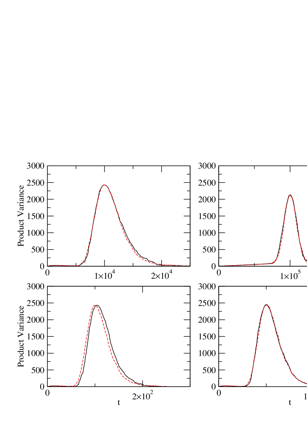
We conclude this section with some remarks. The condition has a physical interpretation: it corresponds to the situation in which the concentrations are very low. Indeed is the only rate that depends on the volume since it is essentially determined by the search time. Conversely, the condition corresponds to large concentrations. This means that all the four cases we discuss are, in general, experimentally accessible. This kind of approach may be useful in the study of enzymatic reactions inside the cells. Such reactions are often characterized by low number of molecules [3], and probably the Michaelis-Menten picture is appropriate even with a low number of substrate molecules. On the other hand, one can study situations in which concentrations are very high, or cases in which the changes that can occur in the cell environment, for example as a response to a rapidly varying external signal [24], can bring the reaction outside the steady state regime and make a description of this kind more appropriate.
V Conclusions
In this paper we introduced a general method for the decimation of “fast modes” in systems evolving according to a Master equation via a coarse graining procedure. Our method is general, and somehow, in the spirit of the renormalization group (RG) approach. Indeed, similar approaches have been proposed in statistical mechanics for the study of disordered systems [25]. At variance with the RG, we do not aim at reaching a fixed point by repeating the decimation procedure. In general, the method is applied only once: a sensible value of the parameter , which selects the coarse graining level, may be easily chosen by looking at the magnitude of the total out rates .
We show that the procedure is commutative and brings to consistent results for a general master equation, independently of the dimensionality. However, for the sake of simplicity, we discussed in details low dimensional examples, where the method brings also to analytical predictions. In the discrete version of the double well potential, the decimation procedure is able to reproduce the well known result for the transition time. A numerical analysis shows that the method gives a very good approximation of the original system in the case of a random walk with defects. In the case of an enzymatic reaction, we show that the method allows for predictions only in some well defined limiting cases. However, in these cases, the prediction are more general than those obtained within a steady-state approximation.
Let us conclude with a short comparison with other approaches to multiscale master equations. Our method is more similar in spirit to projection methods[16, 17] than to other quasi-steady states methods [18, 19]. The reason is that the result of our procedure is still a master equation while the other method describe the fast dynamics in a different way (with a differential or Langevin equation). The main difference between our method and the finite state projection is that our procedure is “local” (we consider fast and slow states) while projection methods generally consider eigenvalues and eigenvector of the transition matrix. Projection methods are usually of more general applicability, however our procedure may allow a more transparent interpretation of the surviving states, as we show in the examples we considered.
On the other hand, fast variables elimination methods [14, 15] aim at writing an evolution equation for the probability of slow states summed over the probability of the fast ones. In this way one loses informations about the fast states and, if there is separation of scales, may write a closed equation for the slow ones. We show that our approach does not imply such coarse graining. In fact, no information about the fast states is lost in our case and their dynamics can be reconstructed after solving the problem involving the slow states only.
There are also analogies between our method and some coarse graining procedure that have been proposed in the field of complex networks. In this field, a relevant problem is the identification of communities [26] and a possible way to do it is to consider a diffusion process on the network and try to coarse grain the graph while keeping the long timescale properties of this dynamics [28, 27]. The difference is that in these cases the procedure allows for a spatial simplification of the links, while our decimation procedure in a system whose states are seen as elements of a graph brings a suppression of the fast states but without a relevant simplification of the surviving connections.
Appendix: proof of equality (18) and commutativity in
In this appendix we prove that, when decimating a cluster of consecutive states, the product of their out rates can be written as:
| (28) |
remembering the convention that the product of less than one object is equal to one, and it is independent of the order of decimation.

We will show that the above formula holds when decimating states in consecutive order, say from state one after the other to state (see Fig.(8)), remembering that the result does not depend on the order of decimation due to the commutative property. We will demonstrated it by induction: first of all, the above formula is obviously true for :
| (29) |
Now we show that if the equality holds for a given value of , then it holds also for :
which is exactly the same expression of eq.(28) for . This completes our proof.
Acknowledgements.
We are grateful to M. Cencini and A. Puglisi for useful remarks and a detailed reading of the manuscript. A.V. wishes to thank Universitad de las Islas Baleares (Palma de Mallorca, Spain) for hospitality during the first stage of this work. S.P. wishes to thank A.D. Jackson for stimulating discussions and help with the commutativity argument.References
- [1] N.G. Van Kampen, Stochastic Processes in Physics and Chemistry, (North Holland, Amsterdam 1990)
- [2] M.O. Stefanini, A. J. McKane and T. J. Newman, Nonlinearity 18 1575-1595 (2005).
- [3] M.B. Elowitz, A.J. Levine, E.D. Siggia, P.S. Swain, Science 297(5584) pp.1183-1186 (2002).
- [4] M.N. Artyomov, J. Das, M. Kardar, and A.K. Chakraborty, Proc. Natl. Acad. Sci. 104 18958-18963 (2007).
- [5] A. J. McKane and T. J. Newman, Phys. Rev. E 70, 041902 (2004).
- [6] W. E and B. Engquist, Notices of the AMS 50, 1062 (2003).
- [7] V.I. Arnold, Méthodes Mathématiques de la Mécanique Classique (Éditions de Moscou, 1976).
- [8] L. Biferale, A. Crisanti, M. Vergassola and A. Vulpiani, Phys. Fluids 7, 2725 (1995).
- [9] J.M. Ziman Electrons and Phonons (Oxford Univ. Press, Oxford, 1960).
- [10] R. Car and M. Parrinello, Phys. Rev. Lett. 55, 2471 (1985).
- [11] D.T. Gillespie, J. Phys. Chem. 81, 2340 (1977).
- [12] C.V. Rao and A.P. Arkin, J. Chem. Phys. 118, 4999 (2003).
- [13] J. Goutsias, J. Chem. Phys. 122, 184102 (2005).
- [14] M. Frankowicz, M. Moreau, P. P. Szczȩsny , J. Tóth and L. Vicente, J. Phys. Chem. 97, 1891-1895 (1993).
- [15] M. Pineda, R. Imbihl, L. Schimansky-Geier, Ch. Zülicke, J. Chem. Phys. 124, 044701 (2006).
- [16] B. Munsky and M. Khammash, J. Chem. Phys. 124, 044104 (2006).
- [17] S. Peles, B. Munsky and M. Khammash, J. Chem. Phys. 125, 204104 (2006).
- [18] E. L. Haseltine and J. B. Rawlings, J. Chem. Phys 117, 6959 (2002).
- [19] Y. Cao, D. Gillespie and L. Petzold, J. Comp. Phys. 206, 395 (2005).
- [20] See e.g. H. Risken, The Fokker-Planck Equation p. 123 (Springer, 1989).
- [21] N. W. Ashcroft and N. D. Mermin, Solid State Physics, pp. 430-433 (Thomson Learning, Toronto, 1976).
- [22] E.H. Lieb and D.C. Mattis, Mathematical Physics in One Dimension, (Academic Press, New York, 1966).
- [23] See e.g. I.H. Segel, Enzyme Kinetics (John Wiley & Sons, 1993).
- [24] G. Tiana, S. Krishna, S. Pigolotti, M.H. Jensen and K. Sneppen, Phys. Biol. 4(2), R1-R17, doi:10.1088/1478-3975/4/2/R01 (2007).
- [25] F. Igloi and C. Monthus, Phys. Rep. 412, 277-431 (2005).
- [26] M. Girvan and M. E. J. Newman, Proc. Natl. Acad. Sci 99(12), 7821-7826 (2002).
- [27] D. Gfeller and P. De Los Rios, Phys. Rev. Lett. 99, 038701 (2007).
- [28] J. Reichardt and S. Bornholdt, Phys. Rev. Lett. 93, 218701 (2004).