Predictions from an anisotropic inflationary era

Cyril Pitrou Email: pitrou@iap.fr Affiliation: Institut d’Astrophysique de Paris, Université Pierre & Marie Curie - Paris VI, CNRS-UMR 7095, 98 bis, Bd Arago, 75014 Paris, France, Thiago S. Pereira Email: thiago@if.usp.br Affiliation: Instituto de Física, Universidade de São Paulo CP 66318, 05315-970 São Paulo, Brazil, Jean-Philippe Uzan Email: uzan@iap.fr Affiliation: Institut d’Astrophysique de Paris, Université Pierre & Marie Curie - Paris VI, CNRS-UMR 7095, 98 bis, Bd Arago, 75014 Paris, France.

18 novembre 2007

Abstract

This article investigates the predictions of an inflationary phase starting from a homogeneous and anisotropic universe of the Bianchi $I$ type. After discussing the evolution of the background spacetime, focusing on the number of $e$ -folds and the isotropization, we solve the perturbation equations and predict the power spectra of the curvature perturbations and gravity waves at the end of inflation.

The main features of the early anisotropic phase is (1) a dependence of the spectra on the direction of the modes, (2) a coupling between curvature perturbations and gravity waves, and (3) the fact that the two gravity waves polarisations do not share the same spectrum on large scales. All these effects are significant only on large scales and die out on small scales where isotropy is recovered. They depend on a characteristic scale that can, but a priori must not, be tuned to some observable scale.

To fix the initial conditions, we propose a procedure that generalises the one standardly used in inflation but that takes into account the fact that the WKB regime is violated at early times when the shear dominates. We stress that there exist modes that do not satisfy the WKB condition during the shear-dominated regime and for which the amplitude at the end of inflation depends on unknown initial conditions. On such scales, inflation loses its predictability.

This study paves the way to the determination of the cosmological signature of a primordial shear, whatever the Bianchi $I$ spacetime. It thus stresses the importance of the WKB regime to draw inflationary predictions and demonstrates that when the number of $e$ -folds is large enough, the predictions converge toward those of inflation in a Friedmann-Lemaître spacetime but that they are less robust in the case of an inflationary era with a small number of $e$ -folds.

pacs

98.80.Cq, 04.62.+v,04.20.cv

I Introduction

Inflation [1, 2] (see Ref. [3] for a recent review of its status) is now one of the cornerstones of the standard cosmological model. In its simplest form, inflation has very definite predictions: the existence of adiabatic initial scalar perturbations and gravitational waves, both with Gaussian statistics and an almost scale invariant power spectrum [4, 5]. Various extensions, which in general involve more fields, allow e.g. for isocurvature perturbations [6], non-Gaussianity [7], and modulated fluctuations [8]. All these features let us hope that future data will shed some light on the details (and physics) of this primordial phase of the universe.

Almost the entire literature on inflation assumes that the universe is homogeneous and isotropic while homogeneity and isotropy are what inflation is supposed to explain. Indeed, the dynamics of anisotropic inflationary universes has been widely discussed [9]. It was demonstrated that under a large variety of conditions, inflation occurs even if the spacetime is initially anisotropic [10], regardless of whether it is dominated by a pure cosmological constant or a slow-rolling scalar field. The isotropization of the universe was even generalized to Bianchi braneworld models [11] recently. It should be emphasized, however, that a deviation from isotropy [10] or flatness [12] may have a strong effect on the dynamics of inflation, and in particular on the number of $e$ -folds.

The study of the perturbations during the isotropization phase has been overlooked, mainly because in the past decades one was mostly focused on large field inflationary models, which generically give very long inflationary phases. This was also backed up by the ideas of chaotic inflation and eternal inflation [3]. In such cases, it is thus an excellent approximation to describe the universe by a Friedmann-Lemaître (FL) spacetime when focusing on the modes observable today since they exited the Hubble radius approximatly in the last 60 $e$ -folds. In this case, the origin of the density perturbations is understood as the amplification of vacuum quantum fluctuations of the inflaton. In particular, the degrees of freedom that should be quantized deep in the inflationary phase, and known as the Mukhanov-Sasaki variables [13], were identified [5], which completely fixes the initial conditions and makes inflation a very predictive theory.

In the context of string theory, constructing a string compactification whose low energy effective Lagrangian is able to produce inflation is challenging (see Ref. [14]). In particular, it has proved to be difficult to build large field models [15] (in which the inflaton moves over large distances compared to the Planck scale in field space). This has led to the idea that, in this framework, an inflationary phase with a small number of $e$ -folds is favored (see however Ref. [16]). If so, the predictions of inflation are expected to be sensitive to the initial conditions, and in particular the classical inhomogeneities are not expected to be exponentially suppressed, which makes the search for large scale deviations from homogeneity and isotropy much more motivated, as well as the possibility that the inflaton has not reached the inflationary attractor. More important, it is far from obvious (as we shall discuss in details later) that all observable modes can be assumed to be in their Bunch-Davies vacuum initially, and more puzzling, that for a given mode modulus the possibility of setting the initial conditions will depend on its direction. If so, then the initial conditions for these modes would have to be set in the stringy phase, an open issue at the time.

The theory of cosmological perturbations in a Bianchi universe was roughed out in Ref. [17, 18, 19] (see also Ref. [20] and Ref. [21] for the case of higher-dimensional Kaluza-Klein models and Ref. [22] for the quantization of test fields and particle production in an anisotropic spacetime). Recently, we performed a full analysis of the cosmological perturbations in an arbitrary Bianchi $I$ universe [23]. It was soon followed by an analysis [24] that focused on Bianchi $I$ universe with a planar symmetry. As we shall see in this work, the case of a planar symmetric spacetime is not generic (both for the dynamics of the background and the evolution of the perturbations).

From a more observationally oriented perspective, the primordial anisotropy can imprint a preferred direction in the primordial power spectra. This could be related to the possible large scale statistical anomalies [25] of the cosmic microwave background (CMB) anisotropies. Many possible explanations have been proposed, including foregrounds [26], non-trivial spatial topology [27] (which implies a violation of global isotropy [28]), the breakdown of local isotropy due to multiple scalar fields [29], the presence of spinors [30] or dynamical vectors [31], the effect of the spatial gradient of the inflaton [32] or a late time violation of isotropy [33]. In the case of universes with planar symmetry, the signatures on the CMB were derived by many authors [24, 34, 35]. In this case, a large primordial shear is indeed necessary, which is not in contradiction with the constraints obtained from the CMB [36] or from the big-bang nucleosynthesis [37]. This brings a secondary motivation to our analysis: can the CMB anisotropy be related to an anisotropic primordial phase or, on the other hand, can it constrain the primordial shear and what are the exact predictions of a primordial anisotropic phase?

This is however not our primary motivation. In the first place, we are interested in understanding the genericity of the predictions of inflation, and in particular with respect to the symmetries of the background spacetime. As we shall see, the simple extension considered in this article drives a lot of questions, concerning both the initial conditions in inflation and, more generally, quantum field theory in curved spacetime.

In this article, we build on our previous work [23] to investigate the dynamics and predictions of one field inflation starting from a generic Bianchi $I$ universe. After discussing the dynamics of the background in § II, we focus on the evolution of the perturbations in § III. In particular, we will need to understand the procedure for the quantization during inflation. As we shall see in § IV, this procedure deviates from the one standardly used in a Friedmann-Lemaître spacetime, and even in a planar symmetric spacetime as discussed in Ref. [24]. The main reason for such an extension lies in the fact that there always exist modes that were not in a WKB regime during the shear-dominated inflationary era. It follows that, while our procedure leads to similar predictions to the standard one on small scales, it appears that there is a lack of predictibility on large scales. Indeed, we do not want to push our description beyond the Planck or string scale where extensions of general relativity have to be considered. This may give a description of both the early phase of the inflationary era and also a procedure to fix the initial conditions without any ambiguity. In § V, we explicitly compute the primordial spectra, for both scalar modes and gravity waves. We will describe in details the effect of the anisotropy and show how the isotropic predictions are recovered on small scales.

II Background dynamics

We first set our notations in § II.1 and describe the dynamics of the background, focusing on its general solutions in § II.2. We then turn to the slow-roll regime and to the case of a massive free field, that we shall use as our working example, respectively in § II.3 and § II.4.

II.1 Definitions and notations

Bianchi spacetimes [38] are spatially homogeneous and those of type $I$ have Euclidean hypersurfaces of homogeneity. In comoving coordinates, and using cosmic time, their metric takes the general form

{\rm d}s^{2}=-{\rm d}t^{2}+\sum_{i=1}^{3}X_{i}^{2}(t)\,\left({\rm d}x^{i}\right)^{2}\ ,

(1)

which includes three a priori different scale factors. It includes the Friedmann-Lemaître spacetimes as a subcase when the three scale factors are equal, and the extensively studied planar symmetric universes when only two of the three scale factors are different. The average scale factor, defined by

S(t)\equiv\left[X_{1}(t)X_{2}(t)X_{3}(t)\right]^{1/3}\,,

(2)

characterises the volume expansion of the universe. The metric (1) can then be recast under the equivalent form

{\rm d}s^{2}=-{\rm d}t^{2}+S^{2}(t)\gamma_{ij}(t){\rm d}x^{i}{\rm d}x^{j}\,,

(3)

where the “spatial metric”, $\gamma_{ij}$ , is the metric on constant time hypersurfaces. It can be decomposed as

\gamma_{ij}=\hbox{exp}\left[{2\beta_{i}(t)}\right]\delta_{ij}\,,

(4)

where the functions $\beta_{i}$ must satisfy the constraint

\sum_{i=1}^{3}\beta_{i}=0\,.

(5)

Let us introduce some useful definitions. First, we consider the scale factors

a_{i}\equiv\hbox{e}^{\beta_{i}(t)}\ ,\qquad X_{i}=Sa_{i}\,.

(6)

They are associated to the following Hubble parameters

H\equiv\frac{\dot{S}}{S}\ ,\qquad h_{i}=\frac{\dot{X}_{i}}{X_{i}}\ ,\qquad\dot{\beta}_{i}=\frac{\dot{a}_{i}}{a_{i}}\ ,

(7)

which are trivially related by

h_{i}=H+\dot{\beta}_{i}\ ,\qquad H=\frac{1}{3}\sum_{i=1}^{3}h_{i}\ ,

(8)

where the dot refers to a derivative with respect to physical time. We define the shear as

\hat{\sigma}_{ij}\equiv\frac{1}{2}\dot{\gamma}_{ij}

(9)

and introduce the scalar shear by

\hat{\sigma}^{2}\equiv\hat{\sigma}_{ij}\hat{\sigma}^{ij}=\sum_{i}\dot{\beta}_{i}^{2}\ .

(10)

(See appendix A of Ref. [23] to see the relation with the shear usually defined in the $1+3$ formalism.) To finish, we define the conformal time by ${\rm d}t\equiv S{\rm d}\eta$ , in terms of which the metric (3) is recast as

{\rm d}s^{2}=S^{2}(\eta)\left[-{\rm d}\eta^{2}+\gamma_{ij}(\eta){\rm d}x^{i}{\rm d}x^{j}\right].

(11)

We define the comoving Hubble parameter by $\mathcal{H}\equiv S^{\prime}/S$ , where a prime refers to a derivative with respect to the conformal time. The shear tensor, now defined as

\sigma_{ij}\equiv\frac{1}{2}\gamma_{ij}^{\prime}\ ,

(12)

is clearly related to $\hat{\sigma}_{ij}$ by $\sigma_{ij}=S\hat{\sigma}_{ij}$ so that $\sigma^{2}\equiv\sigma_{ij}\sigma^{ij}$ is explicitly given by $\sigma^{2}=\sum_{i=1}^{3}(\beta_{i}^{\prime})^{2}$ and is related to its cosmic time analogous by $\sigma=S\hat{\sigma}$ .

II.2 Friedmann equations and their general solutions

II.2.1 Friedmann equations

In cosmic time, assuming a general fluid as matter source with stress-energy tensor

T_{\mu\nu}=\rho u_{\mu}u_{\nu}+P(g_{\mu\nu}+u_{\mu}u_{\nu})+\pi_{\mu\nu},

(13)

where $\rho$ is the energy density, $P$ the isotropic pressure and $\pi_{\mu\nu}$ the anisotropic stress ( $\pi_{\mu\nu}u^{\mu}=0$ and $\pi_{\mu}^{\mu}=0$ ), the Einstein equations take the form

$\displaystyle 3H^{2}$	$\displaystyle=$	$\displaystyle\kappa\rho+\frac{1}{2}\hat{\sigma}^{2}\,,$	(14)
$\displaystyle\frac{\ddot{S}}{S}$	$\displaystyle=$	$\displaystyle-\frac{\kappa}{6}(\rho+3P)-\frac{1}{3}\hat{\sigma}^{2}\,,$	(15)
$\displaystyle(\hat{\sigma}^{i}_{j})^{.}$	$\displaystyle=$	$\displaystyle-3H\hat{\sigma}^{i}_{j}+\kappa\tilde{\pi}^{i}_{j}\,,$	(16)

and the conservation equation for the matter reads

\dot{\rho}+3H(\rho+P)+\hat{\sigma}_{ij}\tilde{\pi}^{ij}=0\,,

(17)

where the $ij$ -component of $\pi_{\mu\nu}$ has been defined as $S^{2}\tilde{\pi}_{ij}$ (so that $\tilde{\pi}^{i}_{j}=\gamma^{ik}\tilde{\pi}_{kj}$ ).

In this work, we focus on inflation and assume that the matter content of the universe is described by a single scalar field so that

T_{\mu\nu}=\partial_{\mu}\varphi\partial_{\nu}\varphi-\left(\frac{1}{2}\partial_{\alpha}\varphi\partial^{\alpha}\varphi+V\right)g_{\mu\nu}\,.

(18)

This implies that

$\displaystyle 3H^{2}$	$\displaystyle=$	$\displaystyle\kappa\left[\frac{1}{2}\dot{\varphi}^{2}+V(\varphi)\right]+\frac{1}{2}\hat{\sigma}^{2}\,,$	(19)
$\displaystyle\frac{\ddot{S}}{S}$	$\displaystyle=$	$\displaystyle-\frac{\kappa}{3}\left[\dot{\varphi}^{2}-V(\varphi)\right]-\frac{1}{3}\hat{\sigma}^{2}\,,$	(20)
$\displaystyle(\hat{\sigma}^{i}_{j})^{.}$	$\displaystyle=$	$\displaystyle-3H\hat{\sigma}^{i}_{j}\ .$	(21)

The last of these equations is easily integrated and gives

\hat{\sigma}^{i}_{j}=\frac{{\cal K}^{i}_{j}}{S^{3}}

(22)

where ${\cal K}^{i}_{j}$ is a constant tensor, $({\cal K}^{i}_{j})^{\cdot}=0$ . This implies that

\hat{\sigma}^{2}=\frac{{\cal K}^{2}}{S^{6}}\,,

(23)

with ${\cal K}^{2}\equiv{\cal K}^{i}_{j}{\cal K}^{j}_{i}$ , from which we deduce that

\dot{\hat{\sigma}}=-3H\hat{\sigma}\,.

(24)

The conservation equation reduces to the Klein-Gordon equation, which keeps its Friedmannian form,

\ddot{\varphi}+3H\dot{\varphi}+V_{\varphi}=0.

(25)

II.2.2 General solutions

Let us concentrate on the particular case in which $\pi_{\mu\nu}=0$ (relevant for scalar fields) and first set

\beta_{i}=B_{i}W(t)\,,

(26)

where $B_{i}$ are constants yet to be determined. Equations (10) and (23) then imply that

\left(\sum B_{i}^{2}\right)\dot{W}^{2}(t)=\frac{{\cal K}^{2}}{S^{6}}\,,

from which we deduce that

W(t)=\int\frac{{\rm d}t}{S^{3}}

(27)

The constraints (5) and (10) imply that the $B_{i}$ must satisfy

\sum_{i=1}^{3}B_{i}=0,\quad\sum_{i=1}^{3}B_{i}^{2}={\cal K}^{2}\,,

(28)

which can be trivially satisfied by setting

B_{i}=\sqrt{\frac{2}{3}}{\cal K}\sin\alpha_{i},\quad{\rm with}\quad\alpha_{i}=\alpha+\frac{2\pi}{3}i,\quad i\in\{1,2,3\}.

(29)

Thus, the general solution is of the form

\beta_{i}(t)=\sqrt{\frac{2}{3}}{\cal K}\sin\left(\alpha+\frac{2\pi}{3}i\right)\times W(t),

(30)

where $S$ is solution of

3H^{2}=\kappa\rho+\frac{1}{2}\frac{{\cal K}^{2}}{S^{6}}.

(31)

Once an equation of state is specified, the conservation equation gives $\rho[S]$ and we can solve for $S(t)$ .

As we shall see, it is convenient to introduce the reduced shear

x\equiv\frac{1}{\sqrt{6}}\frac{\hat{\sigma}}{H}=\frac{1}{\sqrt{6}}\frac{\sigma}{\mathcal{H}}

(32)

in terms of which the Friedmann equation takes the form

(1-x^{2})H^{2}=\frac{\kappa}{3}\rho\ ,

so that the local positivity of the energy density implies that $x^{2}<1$ .

II.2.3 Particular case of a cosmological constant

First, let us consider the case of a pure cosmological constant, $V={\rm constant}$ and $\dot{\varphi}=0$ . This case is relevant for the initial stage of the inflationary period since we expect first the shear to dominate and the field energy density to be dominated by its potential energy. If not, then the field is fast rolling and its energy density behaves as $S^{-6}$ exactly as the square of the shear.

The Friedmann equation now takes the form

H^{2}=V_{0}\left[1+\left(\frac{S_{*}}{S}\right)^{6}\right],

with¹¹ 1 Note the dimensions: $\rho\sim M^{4}$ , $G\sim M^{-2}$ , $H\sim M$ , $\hat{\sigma}\sim M$ , $B_{i}\sim M$ , $W\sim M^{-1}$ , $V_{0}\sim M^{2}$ , $S_{*}\sim M^{0}$ where $M$ is a mass scale. $V_{0}\equiv\kappa V/3$ and $S_{*}\equiv({\cal K}^{2}/6V_{0})^{1/6}$ . It can be easily integrated to get

S(t)=S_{*}\left[\sinh\left(t/\tau_{*}\right)\right]^{1/3}

(33)

where we have introduced the characteristic time

\tau_{*}^{-1}=3\sqrt{V_{0}}\ .

(34)

Thus, we obtain from Eq. (27)

W(t)=W_{0}+\frac{\tau_{*}}{S_{*}^{3}}\log\left[\tanh\left(\frac{t}{2\tau_{*}}\right)\right]\ ,

(35)

where the constant $W_{0}$ can be set to zero (corresponding to the choice of the origin of time). It follows, using that $\sqrt{3/2}{\mathcal{K}}=S_{*}^{3}/\tau_{*}$ , that the directional scale factors behave as

\displaystyle X_{i}

\displaystyle=

\displaystyle S_{*}\left[\sinh\left(\frac{t}{\tau_{*}}\right)\right]^{1/3}\left[\tanh\left(\frac{t}{2\tau_{*}}\right)\right]^{\frac{2}{3}\sin\alpha_{i}}.

(36)

From this expression, we deduce that the directional Hubble parameters evolve as

\displaystyle h_{i}

\displaystyle=

\displaystyle\frac{1}{3\tau_{*}}\frac{1}{\sinh(t/\tau_{*})}\left[2\sin\alpha_{i}+\cosh(t/\tau_{*})\ \right]

(37)

and further that the average Hubble parameter and reduced shear are given by

\displaystyle H

\displaystyle=

\displaystyle\frac{1}{3\tau_{*}}\frac{1}{\tanh(t/\tau_{*})}\,,\qquad x=\frac{1}{\cosh(t/\tau_{*})}\ .

(38)

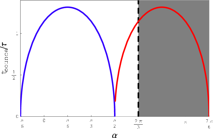
The behaviours of the directional scale factors are depicted on Fig. 1 for various values of the parameter $\alpha$ . We restrict to $\alpha\in[0,2\pi/3]$ and it is clear that for $\alpha<\pi/2$ the $i=3$ direction is bouncing. At $\alpha=\pi/2$ none of the direction is contracting and then it switches to direction $i=2$ , when $\alpha>\pi/2$ . It is thus clear that there is always one bouncing direction, except in the particular case in which $\alpha=\pi/2$ .

Refer to caption — Figure 1: Evolution of the scale factors according to the value of the parameter $\alpha$ . We depict the three directional scale factors and the average scale factor $S$ (dashed line), all in units of $S_{*}$ . The three directional scale factors are permuted when $\alpha$ is changed by $2\pi/3$ . Note that there exist two particular cases in which the spacetime has an extra rotational symmetry when $\alpha=\pi/6$ or $\alpha=\pi/2$ . The latter case is even more peculiar since this is the only Bianchi $I$ universe for which none of the direction is bouncing.

As a first conclusion, let us compute the time at which the contracting direction bounces. Fig 2 (left) depicts the value of the time of the bounce as a function of $\alpha$ and we conclude that it is always smaller than $1.4\tau_{*}$ .

II.2.4 Behaviour close to the singularity

Whatever the potential chosen for the inflaton, the Friedmann equation will be dominated by the shear close to the singularity, so that we can use the solutions obtained in the case of a pure cosmological constant for the sake of the discussion. From the previous analysis, we obtain that

\displaystyle X_{i}

\displaystyle=

\displaystyle S_{*}\left(\frac{t}{2\tau_{*}}\right)^{\frac{2}{3}\sin\alpha_{i}+\frac{1}{3}}\left[1+\frac{1}{18}(1-\sin\alpha_{i})\left(\frac{t}{\tau_{*}}\right)^{2}+\mathcal{O}\left(\left(\frac{t}{\tau_{*}}\right)^{4}\right)\right].

(39)

The metric can thus be expanded around a Kasner solution of the form

{\rm d}s^{2}_{{}_{\rm Kasner}}=-{\rm d}t^{2}+S_{*}^{2}\sum_{i=1}^{3}\left(\frac{t}{2\tau_{*}}\right)^{2p_{i}}({\rm d}x^{i})^{2}

(40)

with the indices

p_{i}(\alpha)=\frac{2}{3}\sin\alpha_{i}+\frac{1}{3}\ ,

(41)

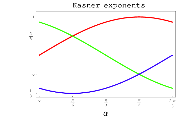
that clearly satisfy $\sum p_{i}=\sum p_{i}^{2}=1$ [see Fig. 2 (right)]. We thus have

{\rm d}s^{2}\simeq-{\rm d}t^{2}+S_{*}^{2}\sum_{i=1}^{3}\left(\frac{t}{2\tau_{*}}\right)^{2p_{i}}\left[1+\frac{1}{12}(1-p_{i})\left(\frac{t}{\tau_{*}}\right)^{2}\right]({\rm d}x^{i})^{2}

(42)

up to terms of order $(t/\tau_{*})^{4}$ .

The invariants of the metric behave as

$\displaystyle R$	$\displaystyle=$	$\displaystyle\frac{4}{3\tau_{*}^{2}}\ ,$	(43)
$\displaystyle R_{\mu\nu}R^{\mu\nu}$	$\displaystyle=$	$\displaystyle\frac{4}{9\tau_{*}^{2}}\ ,$	(44)
$\displaystyle R_{\mu\nu\rho\sigma}R^{\mu\nu\rho\sigma}$	$\displaystyle=$	$\displaystyle\frac{1}{27\tau_{}^{2}}\left\{8+\frac{4}{\cosh^{4}\left[t/(2\tau_{})\right]}\,+\right.$	(45)
		$\displaystyle\qquad\quad\left.+\frac{32\cosh\left(t/\tau_{}\right)}{\sinh^{4}\left(t/\tau_{}\right)}\left[3\cos(\alpha)^{2}\sin(\alpha)-\sin(\alpha)^{3}+1\right]\right\}\ .$	(45)

Clearly, we see that $R$ and $R_{\mu\nu}R^{\mu\nu}$ are regular at the singularity, which is expected for a cosmological constant dominated universe since $R_{\mu\nu}=-\Lambda g_{\mu\nu}$ . The third invariant $R_{\mu\nu\rho\sigma}R^{\mu\nu\rho\sigma}$ diverges when we are approaching the singularity, the only exception being the case where $\alpha=\pi/2$ which corresponds to the positive branch considered in Ref. [24]. In this particular case, the Kasner metric has exponents $(1,0,0)$ . We emphasize that the spacetime $\alpha=\pi/2$ is a singular point in the set of Bianchi spacetimes since there is no uniform convergence of the invariants of the metric evaluated on the singularity when $\alpha\rightarrow\pi/2$ .

II.3 Slow roll parameters

In order to discuss our results, we introduce the slow-roll parameters in the usual way by

\epsilon\equiv 3\frac{\varphi^{\prime 2}}{\varphi^{\prime 2}+2S^{2}V}\,,\qquad\delta\equiv 1-\frac{\varphi^{\prime\prime}}{\mathcal{H}\varphi^{\prime}}=-\frac{\ddot{\varphi}}{H\dot{\varphi}}\,\,.

(46)

With these definitions, the Friedmann and Klein-Gordon equations take the form

(1-x^{2})\mathcal{H}^{2}=\frac{\kappa}{3-\epsilon}VS^{2}\,,\qquad(3-\delta)\mathcal{H}\varphi^{\prime}+V_{\varphi}S^{2}=0\,,

(47)

and we deduce that

\frac{\mathcal{H}^{\prime}}{\mathcal{H}^{2}}=(1-\epsilon)+\left(\epsilon-3\right)x^{2}\,,

(48)

so that

\frac{S^{\prime\prime}}{S}=\mathcal{H}^{2}\left[2-\epsilon+\left(\epsilon-3\right)x^{2}\right]

(49)

and

\epsilon^{\prime}=2\mathcal{H}\epsilon(\epsilon-\delta)\,.

(50)

Interestingly, it is easy to check that

x^{\prime}=-\mathcal{H}x(1-x^{2})(3-\varepsilon)\ ,

from which we deduce that

\delta^{\prime}=\mathcal{H}\left[-9x^{2}+\frac{S^{2}V_{,\varphi\varphi}}{\mathcal{H}^{2}}-(1-x^{2})(3\epsilon+3\delta)+\delta(\delta+\epsilon(1-x^{2}))\right]\ .

(51)

From the definition (46) and making use of the second equation of Eqs. (47), we deduce that the slow-roll $\epsilon$ parameter takes the form

\epsilon=\frac{(1-x^{2})}{2\kappa}\left(\frac{V_{,\varphi}}{V}\right)^{2}\left(\frac{3-\epsilon}{3-\delta}\right)^{2}\,.

Once we use the relation $\dot{\varphi}^{2}=2\epsilon V/(3-\epsilon)$ , we deduce that

\dot{\varphi}=-\frac{1}{\sqrt{\kappa}}\sqrt{\frac{(3-\epsilon)(1-x^{2})}{(3-\delta)^{2}}}\frac{V_{,\varphi}}{\sqrt{V}}\ .

(52)

As long as $\dot{\varphi}^{2}\ll V(\varphi)$ and in the limit $x\rightarrow 1$ , which corresponds to the shear dominated period prior to the inflationary phase, we have that

\epsilon\rightarrow 0\ ,\qquad\delta\rightarrow-3\ ,

(53)

but we still have $\delta^{\prime}\rightarrow 0$ . It follows that initially, even if the shear decreases rapidly, $\varphi$ remains almost constant and $\delta$ remains close to $-3$ . This solution converges when $t\rightarrow 0$ to the pure cosmological constant solution of §II.2.3. Note that this conclusion differs from the statement of Ref. [39].

Before, we reach the slow-roll attractor, we may be in a transitory regime in which $\dot{\varphi}^{2}\gg V$ . Then, this implies that

\epsilon\rightarrow 3,\quad\delta\rightarrow 3,\quad\dot{\varphi}\simeq\frac{\varphi_{0}}{t}\ .

The field velocity decreases so that this solution converges rapidly toward the slow-rolling attractor. These general results on the limiting behaviours will be important to understand the dynamics of the inflaton.

II.4 Numerical integration for a massive scalar field

In this article, we will consider the explicit example of chaotic inflation with a potential

V=\frac{1}{2}m^{2}\varphi^{2}\,.

(54)

The dynamical equations (19) and (25) can be rescaled as

	$\displaystyle h^{2}=\frac{1}{6}\left[\frac{1}{2}\dot{\psi}^{2}+\psi^{2}+\left(\frac{S_{*}}{S}\right)^{6}\right]$		(55)
	$\displaystyle\ddot{\psi}+3h\dot{\psi}+\psi=0\ ,$		(56)

where we use $\tau=mt$ as a time variable (so that $h=H/m$ ), $\psi=\varphi/M_{p}$ (with $M_{p}^{-2}=8\pi G=\kappa$ ) as the field variable, and where $S_{*}=({\cal K}/m)^{1/3}$ . Under this form, it is clear that the various solutions of the system (55-56) are, in general, characterised by the three numbers $\{\psi(t_{0}),\dot{\psi}(t_{0}),S_{*}\}$ . As we will now see, this extra dependence on the parameter $S_{*}$ causes our dynamical system to behave differently from its analogous in Friedmann-Lemaître spacetimes²² 2 There is another way to see this: the term in $S^{-6}$ in Eq. (55) is equivalent to the contribution of a massless scalar field, $\chi$ say, that would satisfy the Klein-Gordon equation $\ddot{\chi}+3h\dot{\chi}=0$ , implying $\dot{\chi}\propto S^{-3}$ . One requires initial conditions for this extra-degree of freedom as well.. Under this form, we also see clearly that one cannot continuously go from a Bianchi to a FL spacetime (because either $S_{*}=0$ or $S_{*}\neq 0$ ), even though Bianchi spacetime isotropizes.

It is well known that the dynamics of the inflationary stage in a Friedmann-Lemaître spacetime is characterised by attractor solutions, clearly seen in the phase space. For a large set of initial conditions, the solutions converge to the slow-roll stage defined by an almost constant $\dot{\varphi}$ and $\varphi$ decreasing accordingly. It is thus given by a roughly horizontal line in the phase portrait which ends with the oscillations of the scalar field at the bottom of its potential. As previously mentioned, the slow-roll inflationary stage in Bianchi $I$ spacetimes possesses the same attractor behaviour, although it is quite different during the initial shear-dominated phase. When the shear dominates, the solutions are rapidly attracted to the point $\dot{\varphi}\simeq 0$ and $\varphi$ nearly constant. This is the attractor whose solution is given by Eqs. (58-62). It then converges towards the Friedmann-Lemaître behaviour when the shear becomes negligible (see Fig. 4).

In conclusion, we have a double attraction mechanism, namely of the field dynamics toward the slow-roll attractor and of the Bianchi spacetime toward a Friedmann-Lemaître solution.

In Fig. 5, we compare the dynamics of the inflationary phase of a Bianchi $I$ and a Friedmann-Lemaître spacetimes. While in both cases the (average) scale factors grow, the effect of a shear-dominated phase is to initially decrease the velocity of the expansion of the Bianchi universe. On the other hand, the dynamics of the scalar field is barely affected by the presence of the shear as long as we have reached the slow-roll attractor. In the following we will assume that we have reached this attractor. If the number of $e$ -folds is small, it is not clear that this attractor has been reached, regardless of whether or not we assume a Friedmann-Lemaître spacetime. In such a case, one has to rely on families of trajectories to draw the observational predictions (see e.g. Ref. [40]).

Let us now consider the behaviour close to the singularity and introduce the characteristic time $\tau_{*}$ , explicitly given by

\tau_{*}=\sqrt{\frac{2}{3}}\frac{M_{p}}{m\varphi_{0}}\ .

(57)

By developing all the previous equations in powers of $t/\tau_{*}$ , we obtain that

$\displaystyle H(t)$	$\displaystyle=$	$\displaystyle\frac{1}{3t}\left[1+\frac{1}{3}\frac{t^{2}}{\tau_{}^{2}}+\mathcal{O}\left(\frac{t^{4}}{\tau_{}^{4}}\right)\right]\ ,$	(58)
$\displaystyle x(t)$	$\displaystyle=$	$\displaystyle 1-\frac{1}{2}\frac{t^{2}}{\tau_{}^{2}}+\mathcal{O}\left(\frac{t^{4}}{\tau_{}^{4}}\right)\ ,$	(59)
$\displaystyle\varphi(t)$	$\displaystyle=$	$\displaystyle\varphi_{0}\left[1-\frac{1}{6}\left(\frac{M_{p}}{\varphi_{0}}\right)^{2}\frac{t^{2}}{\tau_{}^{2}}+\mathcal{O}\left(\frac{t^{4}}{\tau_{}^{4}}\right)\right]\ ,$	(60)
$\displaystyle\delta(t)$	$\displaystyle=$	$\displaystyle-3\left[1-\frac{1}{2}\frac{t^{2}}{\tau_{}^{2}}+\mathcal{O}\left(\frac{t^{4}}{\tau_{}^{4}}\right)\right]\ ,$	(61)
$\displaystyle\epsilon(t)$	$\displaystyle=$	$\displaystyle\frac{1}{3}\left(\frac{M_{p}}{\varphi_{0}}\right)^{2}\frac{t^{2}}{\tau_{}^{2}}+\mathcal{O}\left(\frac{t^{4}}{\tau_{}^{4}}\right)\ ,$	(62)

in complete agreement with the expansions obtained in Ref. [24]. In this limit, we understand why $\delta\rightarrow-3$ close to the singularity. It simply reflects the fact that the field decreases as $t^{2}$ . This is different from the case of chaotic inflation in a Friedmann-Lemaître spacetime where the field varies linearly with time during the slow-roll regime since in that case

\displaystyle\varphi=\varphi_{i}\left[1-\left(\frac{M_{p}}{\varphi_{i}}\right)^{2}\frac{t}{\tau_{*}}\right]\ ,\qquad S=S_{i}\,\exp\left\{{\frac{1}{M_{p}^{2}}[\varphi_{i}^{2}-\varphi^{2}(t)]}\right\}\ ,

and the slow-roll parameters are explicitly given by

\epsilon=2\frac{M_{p}^{2}}{\varphi^{2}}\ ,\qquad\delta=0\ .

Let us come back on the slow-roll parameters defined in § II.3. In the particular case of a quadratic potential, we have

\delta^{\prime}=\mathcal{H}(3-\delta)\left[\frac{\epsilon^{2}-3\delta}{3-\epsilon}-x^{2}(3-\epsilon)\right]\ ,

(63)

since $S^{2}V_{,\varphi\varphi}=\epsilon{\mathcal{H}^{2}}(3-\delta)^{2}/(3-\epsilon)$ . During the shear-dominated phase, $\delta\sim-3$ and the previous equation tells us that $\delta$ remains constant. It follows from Eq. (50) that $\epsilon^{\prime}$ is of the same order than $\epsilon$ (note the difference between the standard case in which $\epsilon^{\prime}$ is second order). It follows that the variation of $\epsilon$ cannot be neglected until $\delta$ has converged toward $0$ . Then $\epsilon$ can be considered as constant until the end of inflation. While the universe isotropizes, both $\delta$ and $\epsilon$ converged toward their Friedmann-Lemaître value. Fig. 6 illustrates the evolution of the two slow-roll parameters and compare them to their values in a Friedmann-Lemaître universe.

For any initial value of the scalar field, $\varphi_{0}$ , we define $\varphi_{i}$ as the value of the field when the universe starts to inflate, that is at the time when $\ddot{S}=0$ . Then, the number of $e$ -folds of the inflationary period is defined as

N[\varphi_{i}]\equiv\ln\frac{S(\varphi_{f})}{S(\varphi_{i})}=\int_{\varphi_{i}}^{\varphi_{f}}\frac{H}{\dot{\varphi}}{\rm d}\varphi\ ,

(64)

where $\varphi_{f}$ is the value of the field at which $\epsilon=1$ . Since at that time the shear is negligible, $\varphi_{f}$ is given by

\varphi_{f}=\sqrt{2}M_{p}\ .

(65)

It follows that for any initial value of the field, we can characterise the shear-dominated phase by

\Delta\varphi[\varphi_{0}]=\varphi_{0}-\varphi_{i}[\varphi_{0}]\ ,

(66)

which indicates by how much the field has moved prior to inflation. Then, the duration of the inflationary phase is given

N[\varphi_{0}]=\int_{\varphi_{i}(\varphi_{0})}^{\sqrt{2}M_{p}}\frac{H}{\dot{\varphi}}{\rm d}\varphi\ .

(67)

This has to be compared with the number of $e$ -folds in the FL case

N_{\rm FL}[\varphi_{i}]=\frac{1}{4}\left(\frac{\varphi_{i}}{M_{p}}\right)^{2}-\frac{1}{2}\ .

In Fig. 7 (left), we depict the fractional duration of the shear-dominated phase [see Eq. (66)] as a function of $\varphi_{0}$ . We see that the larger the initial value of the field, the smaller the impact of the shear. Also shown in Fig. 7 is the number of $e$ -folds for the Friedmann-Lemaître and Bianchi spacetimes. The presence of the shear slightly increases the number of $e$ -folds (solid red line in Fig. 7).

II.5 Discussion

This general study of the background shows that generically there is always one bouncing direction, except in the particular case $\alpha=\pi/2$ considered in Ref. [24] (positive branch). Regarding the dynamics of the universe, the expansions (58-62) at lowest order exactly reproduce the exact (numerical) solutions.

This analysis actually shows that the shear is effective typically until the characteristic time $\tau_{*}$ . Going backward in time, the universe goes rapidly to an initial singularity and is thus past incomplete (in fact as other inflationary models [41]). Indeed, as we shall discuss later, we do not want to extrapolate such a model up to the Planck or string times and we just assume that they are a good description of the inflating universe after this time.

We have focused on the evolution of the “slow-roll” parameters and concluded that the variation of $\epsilon$ cannot be neglected until the shear has decayed. We have also shown that the scalar field barely moves during the shear dominated era and that, with same initial value for the scalar field, the number of $e$ -folds is almost not affected (even though slightly larger) by a non-vanishing shear.

III Summary of the perturbation theory

In our previous work [23], we investigated the theory of cosmological perturbations around a Bianchi $I$ universe. We shall now briefly summarize the main steps which are necessary to deduce the dynamical system of equations that we want to solve in this article.

III.1 Mode decomposition

First, we pick up a comoving coordinates system, $\{x^{i}\}$ , on the constant time hypersurfaces. Any scalar function can then be decomposed in Fourier modes as

f\left(x^{j},\eta\right)=\int\frac{{\rm d}^{3}k_{i}}{\left(2\pi\right)^{3/2}}\,\hat{f}\left(k_{i},\eta\right)\,\hbox{e}^{\mathrm{i}k_{i}x^{i}}\,.

(68)

In the Fourier space, the comoving wave co-vectors $k_{i}$ are constant, $k_{i}^{\prime}=0$ . We now define $k^{i}\equiv\gamma^{ij}k_{j}$ that is obviously a time-dependent quantity. Contrary to the standard Friedmann-Lemaître case, we must be careful not to trivially identify $k_{i}$ and $k^{i}$ , since this does not commute with the time evolution. Note however that $x_{i}k^{i}=x^{i}k_{i}$ remains constant.

Besides, since $(k^{i})^{\prime}=-2\sigma^{ip}k_{p}$ , the modulus of the comoving wave vector, $k^{2}=k^{i}k_{i}=\gamma^{ij}k_{i}k_{j}$ , is now time-dependent and its rate of change is explicitly given by

\frac{k^{\prime}}{k}=-\sigma^{ij}\hat{k}_{i}\hat{k}_{j}\ ,

(69)

where we have defined the unit vector

\hat{k}_{i}\equiv\frac{k_{i}}{k}\ .

(70)

Now, we introduce the base $\{e^{1},e^{2}\}$ of the subspace perpendicular to $k^{i}$ . By construction, it satisfies the orthonormalisation conditions

e^{a}_{i}k_{j}\gamma^{ij}=0\ ,\qquad e^{a}_{i}e^{b}_{j}\gamma^{ij}=\delta^{ab}\ .

Such a basis is indeed defined up to a rotation about the axis $k^{i}$ . These two basis vectors allow to define a projection operator onto the subspace perpendicular to $k^{i}$ as

P_{ij}\equiv e_{i}^{1}e_{j}^{1}+e_{i}^{2}e_{j}^{2}=\gamma_{ij}-\hat{k}_{i}\hat{k}_{j}\ .

(71)

It trivially satisfies $P^{i}_{j}P^{j}_{k}=P^{i}_{k}$ , $P^{i}_{j}k^{j}=0$ and $P^{ij}\gamma_{ij}=2$ .

Any symmetric tensor $\bar{V}_{ij}$ that is transverse and trace-free has only two independent components and can be decomposed as

\bar{V}_{ij}(k_{i},\eta)=\sum_{\lambda=+,\times}V_{\lambda}(k^{i},\eta)\,\varepsilon_{ij}^{\lambda}(\hat{k}_{i})\ ,

(72)

where the polarization tensors have been defined as

\varepsilon_{ij}^{\lambda}=\frac{e_{i}^{1}e_{j}^{1}-e_{i}^{2}e_{j}^{2}}{\sqrt{2}}\delta^{\lambda}_{+}+\frac{e_{i}^{1}e_{j}^{2}+e_{i}^{2}e_{j}^{1}}{\sqrt{2}}\delta^{\lambda}_{\times}\,.

(73)

It can be checked that they are traceless ( $\varepsilon_{ij}^{\lambda}\gamma^{ij}=0$ ), transverse ( $\varepsilon_{ij}^{\lambda}k^{i}=0$ ), and that the two polarizations are perpendicular ( $\varepsilon_{ij}^{\lambda}\varepsilon^{ij}_{\mu}=\delta^{\lambda}_{\mu}$ ). This defines the two tensor degrees of freedom.

III.2 Decomposition of the shear

It is then fruitful to decompose the shear in a local basis adapted to the mode that we are considering. The shear being a symmetric trace-free tensor, it can be decomposed on the basis $\{\hat{k}_{i},e^{1}_{i},e^{2}_{j}\}$ as

\sigma_{ij}=\frac{3}{2}\left(\hat{k}_{i}\hat{k}_{j}-\frac{1}{3}\gamma_{ij}\right)\sigma_{{}_{\parallel}}+2\sum_{a=1,2}\sigma_{{}_{\rm V}a}\,\hat{k}_{(i}e^{a}_{j)}+\sum_{\lambda=+,\times}\sigma_{{}_{\rm T}\lambda}\,\varepsilon^{\lambda}_{ij}.

(74)

This decomposition involves 5 independent components in a basis adapted to the wavenumber $k_{i}$ . We must however stress that $(\sigma_{{}_{\parallel}},\sigma_{{}_{\rm V}a},\sigma_{{}_{\rm T}\lambda})$ do not have to be interpreted as the Fourier components of the shear, even if they explicitly depend on $k_{i}$ . This dependence arises from the local anisotropy of space.

Using Eq. (74), it is easily worked out that $\sigma_{ij}\gamma^{ij}=0$ , and that

\sigma_{ij}\hat{k}^{i}=\sigma_{{}_{\parallel}}\hat{k}_{j}+\sum_{a}\sigma_{{}_{\rm V}a}e^{a}_{j}\,,\qquad\sigma_{ij}\hat{k}^{i}\hat{k}^{j}=\sigma_{{}_{\parallel}}\,,

(75)

and

\sigma_{ij}\varepsilon_{\lambda}^{ij}=\sigma_{{}_{\rm T}\lambda}\,,\qquad\sigma_{ij}\hat{k}^{i}e^{j}_{a}=\sigma_{{}_{\rm V}a}\,.

(76)

The scalar shear is explicitly given by

\sigma^{2}=\sigma_{ij}\sigma^{ij}=\frac{3}{2}\sigma_{{}_{\parallel}}^{2}+2\sum_{a}\sigma_{{}_{\rm V}a}^{2}+\sum_{\lambda}\sigma_{{}_{\rm T}\lambda}^{2}\,,

(77)

which is, by construction, independent of $k_{i}$ . We emphasize that the local positivity of the energy density of matter implies [see Eq. (32)] that $\sigma^{2}/6<\mathcal{H}^{2}$ and thus

\frac{1}{2}\sigma_{{}_{\parallel}}\leq\frac{1}{\sqrt{6}}\sigma<\mathcal{H}\,.

(78)

This, in turn, implies that

{\sigma_{{}_{\parallel}}}<2\mathcal{H}\,,

(79)

a property that shall turn to be very useful in the following of our discussion. Analogously, we have that

{\sigma_{{}_{\rm T}\lambda}}<\sqrt{6}\mathcal{H}\,.

(80)

III.3 Gauge invariant variables

We start from the most general metric of an almost Bianchi $I$ spacetime,

{\rm d}s^{2}=S^{2}\left[-\left(1+2A\right){\rm d}\eta^{2}+2B_{i}{\rm d}x^{i}{\rm d}\eta+\left(\gamma_{ij}+h_{ij}\right){\rm d}x^{i}{\rm d}x^{j}\right].

(81)

$B_{i}$ and $h_{ij}$ are further decomposed as

	$\displaystyle B_{i}$	$\displaystyle=$	$\displaystyle\partial_{i}B+\bar{B}_{i}\,,$		(82)
	$\displaystyle h_{ij}$	$\displaystyle\equiv$	$\displaystyle 2C\left(\gamma_{ij}+\frac{\sigma_{ij}}{\mathcal{H}}\right)+2\partial_{i}\partial_{j}E+2\partial_{(i}E_{j)}+2E_{ij}\,,$		(83)

with

\partial_{i}\bar{B}^{i}=0=\partial_{i}E^{i},\quad E_{i}^{i}=0=\partial_{i}E^{ij}.

(84)

We showed, that one can construct the following gauge invariant variables

	$\displaystyle\Phi$	$\displaystyle\equiv$	$\displaystyle A+\frac{1}{S}\left\{S\left[B-\frac{\left(k^{2}E\right)^{\prime}}{k^{2}}\right]\right\}^{\prime}\,,$		(85)
	$\displaystyle\Psi$	$\displaystyle\equiv$	$\displaystyle-C-\mathcal{H}\left[B-\frac{\left(k^{2}E\right)^{\prime}}{k^{2}}\right]\,.$		(86)

for the scalar modes,

\Phi_{i}\equiv\bar{B}_{i}-\gamma_{ij}\left(E^{j}\right)^{\prime}+2\mathrm{i}k^{j}\sigma_{lj}P^{l}_{\,\,i}E,

(87)

for the vector modes and that the tensor mode $E_{ij}$ is readily gauge invariant.

Concerning the matter sector, one can introduce a single gauge invariant variable associated with the scalar field perturbation,

Q\equiv\delta\varphi-\frac{C}{\mathcal{H}}\varphi^{\prime}\ .

(88)

III.4 The Mukhanov-Sasaki variables and their evolution equations

We established that the only degrees of freedom reduce to a scalar mode and two tensor modes

v\equiv SQ\,,\qquad\sqrt{\kappa}\mu_{\lambda}\equiv SE_{\lambda}\ .

(89)

They evolve according to

	$\displaystyle v^{\prime\prime}+\omega^{2}_{v}(k_{i},\eta)v=\sum_{\lambda}\aleph_{\lambda}(k_{i},\eta)\mu_{\lambda}\ ,$		(90)
	$\displaystyle\mu_{\lambda}^{\prime\prime}+\omega^{2}_{\lambda}(k_{i},\eta)\mu_{\lambda}=\aleph_{\lambda}(k_{i},\eta)v+\beth(k_{i},\eta)\mu_{(1-\lambda)}\ ,$		(91)

where the pulsations are explicitly given by

\omega^{2}_{v}(k_{i},\eta)\equiv k^{2}-\frac{z_{\rm s}^{\prime\prime}}{z_{\rm s}}\ ,\qquad\omega^{2}_{\lambda}(k_{i},\eta)\equiv k^{2}-\frac{z_{\lambda}^{\prime\prime}}{z_{\lambda}}\ .

(92)

The two functions $z_{\rm s}$ and $z_{\lambda}$ have been defined by

	$\displaystyle\frac{z_{\rm s}^{\prime\prime}}{z_{\rm s}}(\eta,k_{i})$	$\displaystyle\equiv$	$\displaystyle\frac{S^{\prime\prime}}{S}-S^{2}V_{,\varphi\varphi}+\frac{1}{S^{2}}\left(\frac{2S^{2}\kappa\varphi^{\prime 2}}{2\mathcal{H}-\sigma_{{}_{\parallel}}}\right)^{\prime}\ ,$		(93)
	$\displaystyle\frac{z_{\lambda}^{\prime\prime}}{z_{\lambda}}(\eta,k_{i})$	$\displaystyle\equiv$	$\displaystyle\frac{S^{\prime\prime}}{S}+2\sigma_{{}_{\rm T}(1-\lambda)}^{2}+\frac{1}{S^{2}}\left(S^{2}\sigma_{{}_{\parallel}}\right)^{\prime}+\frac{1}{S^{2}}\left(\frac{2S^{2}\sigma_{{}_{\rm T}\lambda}^{2}}{2\mathcal{H}-\sigma_{{}_{\parallel}}}\right)^{\prime}\ ,$		(94)

and we also need the coupling terms

	$\displaystyle\aleph_{\lambda}(\eta,k_{i})$	$\displaystyle\equiv$	$\displaystyle\frac{1}{S^{2}}\sqrt{\kappa}\left(\frac{2S^{2}\varphi^{\prime}\sigma_{{}_{\rm T}\lambda}}{2\mathcal{H}-\sigma_{{}_{\parallel}}}\right)^{\prime}\ ,$		(95)
	$\displaystyle\beth(\eta,k_{i})$	$\displaystyle\equiv$	$\displaystyle\frac{1}{S^{2}}\left(\frac{2^{2}\sigma_{{}_{\rm T}\times}\sigma_{{}_{\rm T}+}}{2\mathcal{H}-\sigma_{{}_{\parallel}}}\right)^{\prime}-2\sigma_{{}_{\rm T}\times}\sigma_{{}_{\rm T}+}\ .$		(96)

IV Prescription for the initial conditions

The set of equations (90-96) completely determines the evolution of the three degrees of freedom of our problem. To be predictive, we must determine the initial conditions.

In a FL spacetime, the procedure is well understood [5] and relies on the quantization of the canonical variables on sub-Hubble scales where it can be shown that they evolve adiabatically.

We have to understand how far this procedure can be extended to a Bianchi universe and how robust it is to the existence of a non-vanishing primordial shear. We thus start, in § IV.1 by a review of the standard FL procedure, to highlight its hypothesis. In § IV.2, we stress, and also quantify, the differences that appear in a Bianchi universe. This will lead us (§ IV.3) to propose an extension of the quantization procedure. We shall finish in § IV.4 by critically discussing the limits and weaknesses of our quantization procedure.

IV.1 Friedmann-Lemaître universes

For simplicity, let us consider the case of a pure de Sitter phase. This represents no limitation to our following arguments and can be generalised to an almost-de Sitter phase.

IV.1.1 Quantization procedure

In order to be quantized, the canonical variables are promoted to the status of quantum operators [5] and are decomposed as

	$\displaystyle\hat{v}({\bf x},\eta)$	$\displaystyle=$	$\displaystyle\int\frac{{\rm d}^{3}{\bf k}}{(2\pi)^{3/2}}\left[v_{k}(\eta)\hbox{e}^{i{\bf k}.{\bf x}}\hat{a}_{\bf k}+v_{k}^{*}(\eta)\hbox{e}^{-i{\bf k}.{\bf x}}\hat{a}_{\bf k}^{\dagger}\right]\ ,$		(97)
		$\displaystyle\equiv$	$\displaystyle\int\frac{{\rm d}^{3}{\bf k}}{(2\pi)^{3/2}}\left[\hat{v}_{\bf k}(\eta)\hbox{e}^{i{\bf k}.{\bf x}}+\hat{v}_{\bf k}^{\dagger}(\eta)\hbox{e}^{-i{\bf k}.{\bf x}}\right]\ ,$		(97)

where the creation and annihilation operators satisfy the commutation relations $[\hat{a}_{\bf k},\hat{a}_{{\bf k}^{\prime}}^{\dagger}]=\delta^{(3)}({\bf k}-{\bf k}^{\prime})$ . The mode function, $v_{k}(\eta)$ , is solution of the classical Klein-Gordon equation

v_{k}^{\prime\prime}+\omega_{v}^{2}(k,\eta)v_{k}=0\qquad\hbox{with}\qquad\omega_{v}^{2}(k,\eta)=k^{2}-\frac{2}{\eta^{2}}\ ,

(98)

which is the equation of motion for a harmonic oscillator with time-dependent mass, which translates the fact that the field lives in a time-dependent background spacetime. The general solution of Eq. (98) is

v_{k}(\eta)=\left[A(k)H_{\nu}^{(1)}(-k\eta)+B(k)H_{\nu}^{(2)}(-k\eta)\right]\sqrt{-\eta}

where $H_{\nu}$ are the Hankel functions. In the particular case of a de Sitter era considered here, $\nu=3/2$ so that

H_{3/2}^{(2)}(z)=\left[H_{3/2}^{(1)}(z)\right]^{*}=-\sqrt{\frac{2}{\pi z}}\hbox{e}^{-iz}\left(1+\frac{1}{iz}\right)\ .

Canonical quantization consists in imposing the commutation rules $[\hat{v}({\bf x},\eta),\hat{v}({\bf x}^{\prime},\eta)]=[\hat{\pi}({\bf x},\eta),\hat{\pi}({\bf x}^{\prime},\eta)]=0$ and $[\hat{v}({\bf x},\eta),\hat{\pi}({\bf x}^{\prime},\eta)]=\delta^{(3)}({\bf x}-{\bf x}^{\prime})$ on constant time hypersurfaces, $\hat{\pi}$ being the conjugate momentum of $\hat{v}$ . From Eq. (97) and the commutation rules of the annihilation and creation operators, this implies that

v_{k}v_{k}^{\prime*}-v_{k}^{*}v_{k}^{\prime}=i\ ,

(99)

which determines the normalisation of the Wronskian. The choice of a specific mode function $v_{k}(\eta)$ corresponds to the choice of a prescription for the physical vacuum $|0\rangle$ , defined by

\hat{a}_{\bf k}|0\rangle=0\ .

The most natural choice for the vacuum is to pick up the solution that corresponds adiabatically to the usual Minkowsky vacuum so that

v_{k}\rightarrow\frac{1}{\sqrt{2k}}\hbox{e}^{-ik\eta}

when $k\eta\rightarrow-\infty$ . This implies that the mode function is

v_{k}=\frac{1}{\sqrt{2k}}\left(1+\frac{1}{ik\eta}\right)\hbox{e}^{-ik\eta}\ .

(100)

This choice is referred to as the Bunch-Davies vacuum.

IV.1.2 WKB approximation

In more general cases, and for sure in the Bianchi case that follows, we may not have exact solutions for the mode functions. On can redo the previous construction by relying on a WKB approach [42] in which one introduces the WKB mode function

v_{k}^{\rm WKB}(\eta)=\frac{1}{\sqrt{2\omega_{v}}}\hbox{e}^{\pm i\int\omega_{v}{\rm d}\eta}\ .

(101)

It is easily checked that it is solution of

{v_{k}^{\rm WKB}}^{\prime\prime}+\left(\omega^{2}_{v}-Q_{\rm WKB}\right)v_{k}^{\rm WKB}=0

with

Q_{\rm WKB}=\frac{3}{4}\left(\frac{\omega_{v}^{\prime}}{\omega_{v}}\right)^{2}-\frac{1}{2}\frac{\omega_{v}^{\prime\prime}}{\omega_{v}}\ .

(102)

For a function satisfying an equation such as Eq. (98), the WKB solution is thus a good approximation as long as the WKB condition $|Q_{\rm WKB}/\omega_{v}^{2}|\ll 1$ is satisfied. In the example at hand, this condition reduces to $k\eta\rightarrow-\infty$ so that on sub-Hubble scales, the mode function is actually close to its WKB approximation. We see that the quantization procedure thus relies on the fact that there exists an adiabatic (WKB) solution on sub-Hubble scales.

IV.1.3 Primordial spectra on super-Hubble scales

Once the initial conditions are fixed, $v_{k}$ is completely determined and it can then be related to the scalar field perturbation $Q$ (also promoted to the status of operator). After the modes become super-Hubble, i.e. $k\eta\ll 1$ , the scalar field perturbation in flat slicing gauge is given by

\hat{Q}\rightarrow\int\frac{{\rm d}^{3}{\bf k}}{(2\pi)^{3/2}}\,\hat{Q}_{\bf k}\,\hbox{e}^{i{\bf k}.{\bf x}}=\int\frac{{\rm d}^{3}{\bf k}}{(2\pi)^{3/2}}\,\frac{H}{\sqrt{2k^{3}}}\left(\hat{a}_{\bf k}+\hat{a}_{-{\bf k}}^{\dagger}\right)\,\hbox{e}^{i{\bf k}.{\bf x}}\ ,

where we have used that $S(\eta)=-1/H\eta$ for a pure de Sitter inflationary phase, $H$ being a constant in this case. All the modes are proportional to $(\hat{a}_{\bf k}+\hat{a}_{-{\bf k}}^{\dagger})$ so that the variables $\hat{Q}_{\bf k}$ commute. We thus deduce that $\hat{Q}$ has actually the same statistical properties as a Gaussian classical stochastic field. Effectively, we can replace our quantum operators by stochastic fields with Gaussian statistics and we introduce a unit Gaussian random variable, $e_{v}({\bf k})$ , which satisfies

\langle e_{v}({\bf k})\rangle=0\ ,\qquad\langle e_{v}({\bf k})e_{v}^{*}({\bf k}^{\prime})\rangle=\delta^{(3)}({\bf k}-{\bf k}^{\prime})\ .

In this description the mode operators are replaced by stochastic variables according to $\hat{v}_{\bf k}\rightarrow v_{\bf k}=v_{k}(\eta)e_{v}({\bf k})$ and we identify the (quantum) average in the vacuum, i.e. $\langle 0|...|0\rangle$ by an ensemble (classical) average, $\langle...\rangle$ .

The correlation function of $v$ is defined as

\xi_{v}\equiv\langle 0|\hat{v}({\bf x},\eta)\hat{v}({\bf x}^{\prime},\eta)|0\rangle\ ,

and takes the simple form

\xi_{v}=\int\frac{{\rm d}^{3}{\bf k}}{(2\pi)^{3}}|v_{k}|^{2}\hbox{e}^{i{\bf k}.({\bf x}-{\bf x}^{\prime})}\ .

(103)

Interestingly, in a Friedmann universe, isotropy implies that we can integrate over the angle to get

\xi_{v}=\int\frac{{\rm d}k}{k}\,\frac{k^{3}}{2\pi^{2}}|v_{k}|^{2}\,\frac{\sin kr}{kr}\ ,

(104)

and it is , because of the symmetries of the background, a function of $r=|{\bf x}-{\bf x}^{\prime}|$ only. We thus define the power spectra

P_{v}(k)=|v_{k}|^{2}\ ,\qquad{\mathcal{P}}_{v}(k)=\frac{k^{3}}{2\pi^{2}}|v_{k}|^{2}\ .

(105)

In the stochastic picture, the correlator of $v_{\bf k}$ is simply given by

\langle v_{\bf k}v_{{\bf k}^{\prime}}^{*}\rangle=P_{v}(k)\,\delta^{(3)}({\bf k}-{\bf k}^{\prime})\ ,

(106)

from which one easily deduces the power spectrum of the curvature perturbation

P_{\mathcal{R}}(k)=\frac{2\pi^{2}}{k^{3}}{\mathcal{P}}_{\mathcal{R}}(k)=\frac{|v_{k}|^{2}}{z^{2}}\ .

Indeed, we can proceed in the same way for gravity waves. Since they are not coupled to scalar modes and since the two polarisations are independent, we introduce two sets of creation and annihilation of operators, $\hat{b}_{{\bf k},\lambda}$ , one per polarisation. On super-Hubble scales, the two modes can be described by two independent Gaussian classical stochastic fields, $\mu_{{\bf k},\lambda}=\mu_{\bf k}e_{\lambda}({\bf k})$ with

\langle e_{\lambda}({\bf k})e_{\lambda^{\prime}}^{*}({\bf k}^{\prime})\rangle=\delta_{\lambda\lambda^{\prime}}\delta^{(3)}({\bf k}-{\bf k}^{\prime})\ .

The power spectra are thus given by

P_{\lambda}(k)=\frac{2\pi^{2}}{k^{3}}{\mathcal{P}}_{\lambda}(k)=|\mu_{k}|^{2}\ .

Spatial isotropy implies that $P_{+}=P_{\times}$ so that the tensor modes power spectrum is

P_{T}(k)=2\frac{\kappa}{S^{2}}P_{+}(k)\ .

(107)

IV.1.4 Conclusion

To conclude, this short review of the standard procedure highlights (1) the importance of the WKB regime on sub-Hubble scales which allows to construct a Bunch-Davies vacuum adiabatically, (2) the fact that on super-Hubble scales (where one wants to draw the predictions for the initial power spectra) the quantum operators can be conveniently replaced by stochastic fields, (3) the importance of isotropy which implies that there exist 3 independent stochastic directions (because modes are decoupled) and (4) the fact that the two gravity wave polarisations have the same power spectrum.

We shall now see which of these properties generalise to a Bianchi universe.

IV.2 Generic Bianchi $I$ universes

IV.2.1 Characteristic wavenumber

In order to relate our predictions to observations, we introduce the characteristic wavenumber $k_{\rm ref}$ by

k_{\rm ref}\equiv\left.SH\right|_{t=\tau_{*}}\ .

(108)

We define ${\mathcal{N}}$ as the number of $e$ -fold with the quantity $SH$ rather than $S$ in the definition (64). If we denote by ${\mathcal{N}}_{\text{ref}}$ the number of $e$ -folds between $t=\tau_{*}$ and the end of inflation, and ${\mathcal{N}}_{0}$ the number of $e$ -folds from the end of inflation until now, then we can relate $k_{\rm ref}$ to the largest observable scale today, $k_{0}=S_{0}H_{0}$ , by

\frac{k_{\rm ref}}{k_{0}}=e^{({\mathcal{N}}_{0}-{\mathcal{N}}_{\text{ref}})}\,.

(109)

Since during the inflationary era after $\tau_{*}$ , $H$ is nearly constant, then ${\mathcal{N}}_{\text{ref}}\simeq N_{\text{ref}}$ . As for ${\mathcal{N}}_{0}$ , it depends on the post-inflationary evolution and it can be estimated [43] by

\displaystyle{\mathcal{N}}_{0}\simeq 62-\ln\left(\frac{10^{16}\,{\rm GeV}}{V_{k_{0}}^{1/4}}\right)+\frac{1}{4}\ln\frac{V_{k_{0}}}{V_{\rm end}}-\frac{1}{3}\ln\left(\frac{V_{\rm end}^{1/4}}{\rho_{\rm reh}^{1/4}}\right)-\ln h,

(110)

$h$ being the Hubble parameter in units of 100 km.s^-1/Mpc. Typically, $V_{k_{0}}\sim V_{\rm end}$ as long as slow rolling holds. The reheating temperature can be argued to be larger than $\rho_{\rm reh}^{1/4}>10^{10}$ GeV to avoid the gravitino problem [44]. The amplitude of the cosmological fluctuations (typically of order $2\times 10^{-5}$ on Hubble scales) roughly implies that $V_{\rm end}^{1/4}$ is smaller than a few times $10^{16}$ GeV and, for the same reason as above, has to be larger than $10^{10}$ GeV in the extreme case. This implies that $N_{0}$ has approximately to lie between 50 and 70, which is the order of magnitude also required to solve the horizon and flatness problem.

$N_{\rm ref}$ can be computed from the background dynamics, and as shown on Fig. 7, it is almost equivalent to its value in the FL case.

IV.2.2 Anisotropy

The first obvious difference with the FL case arises from the local spatial anisotropy.

First, it is clear from the set of equations (90-91) that it implies that the evolution of the mode functions shall depend on $k_{i}$ and not simply on the modulus. This violation of isotropy will reflect itself on the fact that

1.

the power spectra at the end of inflation will be functions of $\bf k$ and not $k$ , i.e. $P_{v}(k_{i})$ , $P_{\lambda}(k_{i})$ ;
2.

because of the coupling between scalar and gravity waves, there exists a cross-correlation between scalar and tensor, i.e. $\langle v\mu_{\lambda}\rangle\not=0$ ;
3.

the two polarisations shall a priori have two different power spectra, i.e. $P_{+}\not=P_{\times}$ .

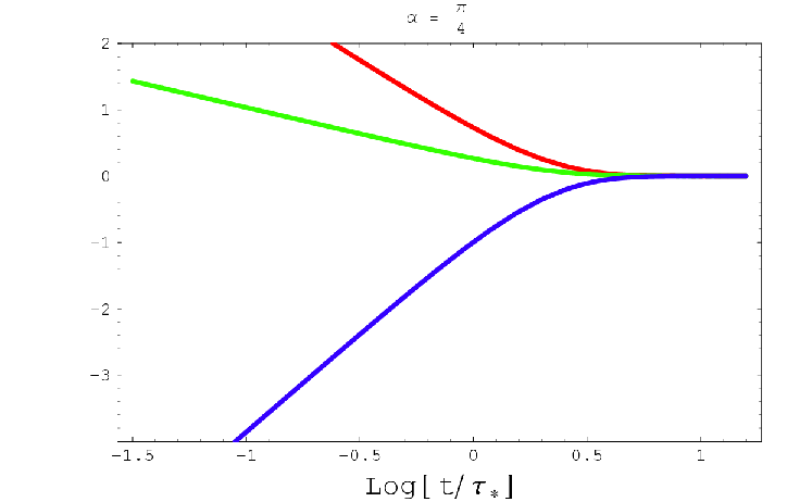
A second related issue arises from the evolution of a comoving wavenumber. Let us consider the different evolutions of a wave-mode of modulus $k$ at the end of inflation according to its orientation. As we see on Fig. 8, depending on its orientation, this mode has very different time evolutions before it settles to a constant value.

IV.2.3 WKB regime

Whatever the Bianchi universe we consider, there is a shear-dominated phase prior to inflation. During this phase $\ddot{S}<0$ . Besides, in a generic Bianchi $I$ spacetime (that is $\alpha\not=\pi/2$ ) two of the scale factors go to zero while the third is bouncing (in the $\alpha=\pi/2$ case, one scale factor goes to zero while the two others remain constant).

For analysing the WKB regime we will consider, as usual, the ratio $k/SH$ to discuss whether a given mode is inside $(k/SH\gg 1)$ or outside $(k/SH\ll 1)$ the Hubble radius. According to the details shown in the Appendix A, if we specify to only one direction we have $k\sim 1/a_{i}\sim S/X_{i}$ , then

\frac{k}{SH}=\frac{1}{X_{i}H}\sim t^{2(1-\sin\alpha_{i})/3}

during the shear-dominated regime. This shows that, except when $\alpha=\pi/2$ , any given mode becomes super-Hubble when we approach the singularity $(t\rightarrow 0)$ , and that this approach is faster (going backwards in time) for modes aligned with the bouncing direction.

In other words, all modes become super-Hubble in the past, and the mode aligned with the bouncing direction (blue line in Fig. 8) becomes super-Hubble earlier (again, going backwards in time) than the ones with same $k$ at the end of inflation but aligned with a growing direction (blue line in Fig. 9).

For these two reasons, we can doubt the existence of a well-defined adiabatic vacuum for all modes through their early evolution, as happens in FL universes. However, we can still ask whether the WKB regime is reached in a short time interval when the shear is not complete negligible, and how long it lasts given the wavenumber.

Let us thus discuss quantitatively the validity of the WKB approximation. First, we focus on the pulsation, we neglect the effect of the couplings, and consider the WKB solutions

v_{\bf k}^{\rm WKB}(\eta)=\frac{1}{\sqrt{2\omega_{v}}}\hbox{e}^{\pm i\int\omega_{v}{\rm d}\eta}\ ,\qquad\mu_{{\bf k},\lambda}^{\rm WKB}(\eta)=\frac{1}{\sqrt{2\omega_{\lambda}}}\hbox{e}^{\pm i\int\omega_{\lambda}{\rm d}\eta}\ .

(111)

They are good approximations of the solutions of Eqs. (90-91) if $|Q_{v,\lambda}^{\rm WKB}/\omega_{v,\lambda}^{2}|\ll 1$ where $Q_{\rm WKB}$ has been defined in Eq. (102).

Fig. 9 illustrates the validity of the WKB approximation for the scalar modes. It depicts the evolution of $|Q_{v}^{\rm WKB}/\omega_{v}^{2}|$ as a function of time for three different modes corresponding to the three principal axis of the Bianchi universe. We see that, for a given comoving wavenumber $k$ at the end of inflation, the WKB condition is always violated in the past and that it is violated first in increasing order of the Kasner coefficients (compare with Fig. 8). It can be checked that the larger the $k$ is, the longer the time during which the WKB condition is restored. For long wavelength modes (typically of order $1/k_{\rm ref}$ ), the WKB regime is never established.

Fig. 10 compares the exact (numerical) solution and the WKB approximation for a mode $k=10k_{\rm ref}$ . Fig. 11 is similar to Fig. 9 but for the tensor modes. Indeed, we reach the same conclusions.

IV.2.4 Couplings

The third difference arises from the coupling between scalar and tensor modes.

As we demonstrated in our previous analysis [23] (see § IV.D), deep in the sub-Hubble regime (that is when $k/SH$ is large enough), the three degrees of freedom decouple and behave as a collection of three independent harmonic oscillators.

However, on larger scales the couplings are a priori non-negligible. We thus need to evaluate with care the scales for which this is a good approximation.

Fig. 12 shows that, while the functions $\aleph_{\lambda}$ , which couple gravity waves and scalar modes can be neglected on small scales, this is certainly not the case for the coupling $\beth$ between the two gravity wave polarizations. This coupling cannot be neglected, even at early time, for modes which are not sub-Hubble enough. Typically, the modes for which this coupling cannot be neglected correspond to modes for which the WKB regime cannot be reached.

Let us compare this situation with the case of multi-field inflation. The equations of evolution for the various scalar field perturbations are also usually coupled (see e.g. Ref. [45] for a recent review). However generally, it is possible to extract independent fields, at least in the sub-Hubble regime [46] so that one can introduce a set of independent stochastic fields. To our knowledge, the situation where this is not possible has not been addressed.

The situation is analogous for us and the long wavelength modes will be particularly difficult to trustfully deal with because they can never be considered as independent.

IV.3 Prescription for setting the initial conditions

IV.3.1 Prescription for Bianchi $I$ spacetimes

It is part of the nature of quantum fluctuations that they do not have initial conditions in the sense that they are continuously excited. As soon as a mode can oscillate, it will be sourced by these quantum fluctuations. Given the discussion of the preceding section, we will thus set the initial conditions at the time where a mode is the deepest in the WKB regime. This time, $t_{i}({\bf k})$ say, depends explicitly on the mode, which is not a problem since all the modes are independent from each other. In practice, we have fixed $t_{i}({\bf k})$ by minimizing $\omega_{v}$ .

As we saw, modes with $k<k_{\rm ref}$ never enter a WKB regime. Given the fact that modes up to approximatively $k_{0}$ have been excited and have, at least as a good approximation, a scale invariant power spectrum, we have to assume that $k_{\rm ref}\lesssim k_{0}$ . Then, from Figs. 13 and 14, we deduce that the WKB is reached for all modes with $k>k_{\rm ref}$ . Indeed this amounts to a fine tuning on the shear such that only the largest observable modes today were affected by the Bianchi phase.

To check the robustness of this procedure, we have varied the time $t_{i}({\bf k})$ . In particular, we have also assumed, as a test, that $t_{i}({\bf k})=\tau_{*}$ for all modes. It can be shown that this does not affect the predictions for the modes with $k\gtrsim 2k_{\rm ref}$ while long wavelength modes are more affected. This is simply due to the fact that the duration of their WKB phase is smaller (see Fig. 16). Also note that the procedure is more robust for the two directions which are not bouncing.

For these modes, and as can be seen from Fig. 15, it is also a good approximation to neglect the coupling terms in Eqs. (90-91). We emphasize that this hypothesis breaks down approximatively at the same time when the WKB approximation also breaks down.

Therefore we will assume that the three modes are independent at the time when they are excited by the quantum fluctuations.

Technically, we thus start our computation by setting

v_{\bf k}=\frac{\hbox{e}^{-i\int\omega_{v}{\rm d}\eta}}{\sqrt{2\omega_{v}({\bf k},\tau)}}\,e_{v}({\bf k})\ ,\qquad{\rm and}\qquad\mu_{\lambda,{\bf k}}=\frac{\hbox{e}^{-i\int\omega_{\lambda}{\rm d}\eta}}{\sqrt{2\omega_{\lambda}({\bf k},\tau)}}\,e_{\lambda}({\bf k})\ ,

(112)

up to an arbitrary relative phase which can be absorbed in the definition of the unit random variables and where the three random variables satisfy

\langle e_{X}({\bf k})e_{Y}^{*}({\bf k}^{\prime})\rangle=\delta_{XY}\delta^{(3)}({\bf k}-{\bf k}^{\prime})\ .

IV.3.2 Freedom in a time redefinition

As mentioned in Ref. [24], the dynamical system of equation for the Mukhanov-Sasaki variables admits time reparameterisations that conserve the canonicity of the system, in the sense that if $v(\eta)$ is a canonical variable that satisfies

\frac{{\rm d}^{2}v}{{\rm d}\eta^{2}}+\omega_{v}^{2}v=0\quad\textrm{and}\quad v\frac{{\rm d}v^{*}}{{\rm d}\eta}-v^{*}\frac{{\rm d}v}{{\rm d}\eta}=i\,,

then there is a function $f$ and a time $\tau$ defined as

f(\eta)^{2}{\rm d}\tau={\rm d}\eta

(113)

through which we can define a new variable $u=fv$ that satisfies

\frac{{\rm d}^{2}u}{{\rm d}\tau^{2}}+\omega_{u}^{2}u=0\quad\textrm{and}\quad u\frac{{\rm d}u^{*}}{{\rm d}\tau}-u^{*}\frac{{\rm d}u}{{\rm d}\tau}=i\,.

If, for example, $v$ is a variable for which the WKB condition does not hold, we might wonder whether exists a function $f$ that would lead to a different conclusion concerning the validity of the WKB condition for the variable $u$ .

In the present case, the transformation Eq. (113) would lead to the same equations of motion satisfied by the new canonical variables

\tilde{v}\equiv fv,\quad\tilde{\mu}_{+}\equiv f\mu_{+},\quad\tilde{\mu}_{\times}\equiv f\mu_{\times}\,,

(114)

where the new pulsations are defined according to

\tilde{\omega}_{v}^{2}\equiv\frac{\omega_{v}^{2}}{f^{4}}-\frac{1}{f}\frac{{\rm d}^{2}f}{{\rm d}\tau^{2}}\,\qquad\tilde{\omega}_{\lambda}^{2}\equiv\frac{\omega_{\lambda}^{2}}{f^{4}}-\frac{1}{f}\frac{{\rm d}^{2}f}{{\rm d}\tau^{2}}\ ,

(115)

and the coupling functions become

\tilde{\aleph}_{\lambda}\equiv\frac{\aleph_{\lambda}}{f^{4}}\ ,\qquad\tilde{\beth}\equiv\frac{\beth}{f^{4}}\ .

(116)

For the sake of simplicity, let us drop $\aleph_{\lambda}$ and $\beth$ in the following discussion. It has been shown in Ref. [24] that, if $\omega_{v}$ and $\omega_{\lambda}$ satisfy the WKB condition, then $f$ is required to satisfy the condition

\frac{1}{f}\left|\frac{{\rm d}^{n}f}{{\rm d}\eta^{n}}\right|\ll\omega_{v}^{n},\omega_{\lambda}^{n}\ ,\qquad\text{with}\quad n=1\ldots 4

(117)

in order for the new equations to also satisfy the WKB condition. Under such conditions, it would lead to the same quantization procedure. Note that the condition for $n=4$ is required when we take $|Q^{\rm WKB}/\omega^{2}|\ll 1$ for the (correct) WKB condition rather than just $\omega^{\prime}/\omega^{2}\ll 1$ , as assumed in Ref. [24].

In our case the pulsations $\omega_{v}$ and $\omega_{\lambda}$ scale like $SH$ when $t\rightarrow 0$ , or like $1/\eta$ in conformal time. Let us choose the integration constant $W_{0}$ of Eq. (35) such that the initial singularity corresponds to $\eta=0$ . Now, if $\omega\simeq C/\eta$ then the associated function $Q_{\rm WKB}$ behaves as

\frac{Q_{\rm WKB}}{\omega^{2}}\simeq-\frac{1}{4C^{2}}\ .

Let us consider now a time redefinition associated to a function $f(\eta)=\eta^{A}$ . Then the WKB condition involves

\frac{\tilde{Q}_{\rm WKB}}{\tilde{\omega}^{2}}\simeq-\frac{\left(A+\frac{1}{2}\right)^{2}}{C^{2}+A(A+1)}\ \ .

(118)

We conclude that it is possible for the WKB condition to be fulfilled with a new time coordinate by choosing $A=-1/2$ , provided $|C|\neq 1/2$ .

Unfortunately, using the expansion (145) and the asymptotic behaviours obtained in Eqs. (53), we deduce that when the leading term of $\omega_{v}^{2}$ is $z_{s}^{\prime\prime}/z_{s}$ , then $\omega_{v}^{2}\rightarrow-\mathcal{H}^{2}$ , which implies that for this pulsation, $|C|=1/2$ .

Thus, it is never possible to construct a time redefinition which would enable the WKB condition to be satisfied for $\tilde{\omega}_{v}$ . The only exception arises when the leading term of $\omega_{v}^{2}$ is $k^{2}$ . This happens for $\alpha=\pi/2$ since in this particular case $k\sim t^{-2/3}\sim\eta^{-1}$ and we recover the conclusions reached in Ref. [24].

As a conclusion, though we might naively think that redefining time could lead to equations satisfying the WKB conditions for the new canonical variables, it is impossible however to build such a change of time coordinates. The choice of the canonical variables is thus unique up to the reparameterisation satisfying the conditions (117), which would not change our predictions.

IV.4 Discussion

Let us discuss our procedure to set the initial conditions.

First for modes smaller than $k_{\rm ref}$ , the WKB regime was never reached. We have no natural prescription to determine their amplitude. A solution, that we do not investigate in this article, would be to fix them by assuming that they minimize their energy, as proposed in Ref. [47] in the study of some trans-Planckian models in which the WKB regime is violated.

On the other hand, and probably in a more conservative way, one could just assume their initial value to be completely random and introduce a free function to describe the initial conditions on large scales. Such a function would then need to be measured from e.g. large angular scale properties of the CMB or predicted by some processes that arise at the Planck or string scale, and that indeed cannot be accounted for in our description.

In the former case, we loose the predictive power on large scales, that actually may just be beyond the actual size of the observable universe. It may seem that we are back to the (historical) pre-inflationary times, where the form of the initial power spectrum of the Harrison-Zel’dovich type had to be postulated in order to reproduce the observations of the large-scale structures. This is somehow a very standard approach in physics in which one learns about the initial conditions of a system by observing its evolution

Inflationary theories allowed to actually predict this spectrum, which makes them very predictive. We realize with this study that these inflationary predictions are very sensitive to the existence of an (classical) initial shear. To recover such a predictive power, we have to hope that a theory handling the dynamics of the universe on this scales [48, 49, 50] or allowing to generate the shear [51] will also provide a better understanding of the initial conditions.

Indeed, one may wonder whether the arbitrary (pre-WKB era) conditions can be amplified and compete in amplitude with the ones of quantum origin seeded during the WKB regime.

To estimate this, note that at early time (apart from the particular case $\alpha=\pi/2$ ), $\omega_{v}^{2}$ behaves as $-z_{s}^{\prime\prime}/z_{s}$ and $\omega_{\lambda}^{2}$ behaves as $-z_{\lambda}^{\prime\prime}/z_{\lambda}$ . The expansion (145) then leads to the conclusion that, at early times,

\omega_{v}^{2}\simeq+\mathcal{H}^{2}\,,

whereas at late time, we deduce from our previous analysis that

\omega_{v}^{2}\simeq-2\mathcal{H}^{2}\ .

Thus, the solutions of Eq. (90) has an oscillatory behaviour until the time when $\omega_{v}=0$ and the arbitrary initial conditions are not amplified. For the tensor modes the situation is different because for some configurations of ${\bf k}$ , we can have $\omega_{\lambda}^{2}\sim-\mathcal{H}^{2}$ at early time, and this leads to an exponential growth. However, since $|\omega_{\lambda}|\lesssim C/\eta$ with $C={\cal O}(1)$ , this exponential growth is typically at most of order

\exp\left(\frac{{\cal O}(1)}{\eta}\times\eta\right)\sim e\ .

It follows that the arbitrary initial conditions either are not amplified or do actually grow, but in the latter case they are amplified by no more than a factor of order unity. We thus expect the transitional tachyonic behaviour and our ignorance of the initial state of the perturbations before the WKB regime not to significantly alter the validity of our prescription for the initial conditions of quantum origin set during the WKB regime.

From a practical point of view, we can estimate the effect of the coupling functions $\aleph$ and $\beth$ by changing their amplitude by hand. We have checked that they hardly affect the predictions that are presented in the following section. In particular, that teaches us that the main directional dependence of the power spectra is induced mainly by the directional dependence of the comoving wavenumbers (see Fig. 8). We have also checked that when $k/k_{\rm ref}$ increases our prediction is similar to the one obtained in standard inflation.

In conclusion, we can trust our prescription for modes larger than $k_{\rm ref}$ and we have to assume (somehow as an observational input) that $k_{\rm ref}<k_{0}$ . This sets a tuning on the primordial shear that we cannot explain with the model at hand. In this regime, we have checked that it is a robust prescription that is not affected by the unknown preexisting perturbations that are completely arbitrary and that fixes the properties of the long wavelength modes.

V Primordial spectra: numerical examples and predictions

V.1 Definition of the spectra

To set the initial conditions as previously detailed, we need to first solve numerically the system (90-91). Because of the couplings, each of the three variables, $v$ and $\mu_{\lambda}$ , will have components along the three independent stochastic directions, even if they were initially independent. For instance,

v_{\bf k}(\eta)=v_{v}({\bf k},\eta)e_{v}({\bf k})+v_{+}({\bf k},\eta)e_{+}({\bf k})+v_{\times}({\bf k},\eta)e_{\times}({\bf k})

and

\mu_{{\bf k}\lambda}(\eta)=\mu_{\lambda v}({\bf k},\eta)e_{v}({\bf k})+\mu_{\lambda\lambda}({\bf k},\eta)e_{\lambda}({\bf k})+\mu_{\lambda(1-\lambda)}({\bf k},\eta)e_{1-\lambda}({\bf k})

and we deduce from the properties of the random variables that

\langle v_{\bf k}(\eta)v_{{\bf k}^{\prime}}^{*}(\eta)\rangle=\left(|v_{v}({\bf k},\eta)|^{2}+|v_{+}({\bf k},\eta)|^{2}+|v_{\times}({\bf k},\eta)|^{2}\right)\delta^{(3)}({\bf k}-{\bf k}^{\prime})\ .

(119)

The power spectrum of the curvature perturbation at the end of inflation (once the shear has decayed away) is thus

P_{\mathcal{R}}({\bf k})=\frac{2\pi^{2}}{k^{3}}{\mathcal{P}}_{\mathcal{R}}({\bf k})=\frac{1}{z_{\rm S}^{2}}\left(|v_{v}({\bf k},\eta)|^{2}+|v_{+}({\bf k},\eta)|^{2}+|v_{\times}({\bf k},\eta)|^{2}\right)\ .

(120)

It can be checked, as expected, that for super-Hubble modes, $\mathcal{R}$ is conserved once the shear is negligible. We thus perform our numerical integration in a time interval long enough so that the universe has been isotropized and all the observable modes have become super-Hubble.

The power spectra of the gravity waves are defined analogously by

P_{\lambda}({\bf k})=\frac{2\pi^{2}}{k^{3}}{\mathcal{P}}_{\lambda}({\bf k})=|\mu_{\lambda v}({\bf k},\eta)|^{2}+|\mu_{\lambda\lambda}({\bf k},\eta)|^{2}+|\mu_{\lambda(1-\lambda)}({\bf k},\eta)|^{2}\ .

(121)

At the beginning of the radiation era, the background spacetime can be described by a Friedmann-Lemaître solution and the primordial anisotropy is now encoded on the statistical properties of the perturbations on large scales. It is thus convenient to decompose the power spectra on spherical harmonics according to

{\mathcal{P}}_{\mathcal{R}}({\bf k})=f_{R}(k)\left[1+\sum_{\ell=1}^{\ell=\infty}\sum_{m=-\ell}^{m=+\ell}r_{\ell m}(k)\,Y_{\ell m}(\hat{\bf k})\right]\ ,

(122)

and

{\mathcal{P}}_{\lambda}({\bf k})=f_{\lambda}(k)\left[1+\sum_{\ell=1}^{\ell=\infty}\sum_{m=-\ell}^{m=+\ell}r^{\lambda}_{\ell m}(k)\,Y_{\ell m}(\hat{\bf k})\right]\ .

(123)

The three functions $f_{R}(k)$ and $f_{\lambda}(k)$ represent the power spectra averaged over the spatial directions,

f_{X}(k)=\int{\mathcal{P}}_{X}({\bf k})\frac{{\rm d}^{2}\hat{\bf k}}{4\pi}\ .

The three series, $r_{\ell m}(k)$ and $r^{\lambda}_{\ell m}(k)$ , characterise the deviation from statistical isotropy. Indeed, we expect the anisotropy to be negligible on small scales, that is

r_{\ell m}(k)\rightarrow 0\qquad\hbox{when}\qquad k\gg k_{\rm ref}\ ,

and that

r_{\ell m}(k)\rightarrow 0\qquad\hbox{when}\qquad\ell\gg 1\ ,

the same being true to $r^{\lambda}_{\ell m}(k)$ . Additionaly, because of the symmetries of the spectrum, the only non-vanishing coefficients are obtained for even $\ell$ and even $m$ . It can also be checked that these coefficients are real and that their values do not depend on the sign of $m$ . Thus, we conclude that there are only $1+\ell/2$ independent real coefficients,

r_{\ell m}\in\mathbb{R}\,\qquad\ell=2\ell^{\prime}\ ,\,m=2m^{\prime}\ ,\quad m^{\prime}=0\ldots\ell^{\prime}\ .

The gravity waves and curvature perturbation are also correlated so that

\langle v_{\bf k}(\eta)\mu_{\lambda{\bf k}^{\prime}}^{*}(\eta)\rangle=\left(|v_{v}\mu_{\lambda v}|+|v_{\lambda}\mu_{\lambda\lambda}|+|v_{(1-\lambda)}\mu_{\lambda(1-\lambda)}|\right)\delta^{(3)}({\bf k}-{\bf k}^{\prime})\ .

(124)

V.2 Predictions

To illustrate the signatures of a Bianchi $I$ inflationary era, we consider a Bianchi spacetime with $\alpha=\pi/4$ . We fix the initial value $\varphi_{0}/M_{p}=3.25\sqrt{8\pi}\simeq 16.3$ for the inflaton field. This implies that the number of $e$ -folds of the accelerating phase is $N[\varphi_{i}]\simeq 67$ . We also set the reference wavenumber to $k_{\rm ref}\simeq 157m\simeq 157~10^{-6}M_{P}$ . This corresponds to the definition (108) evaluated with the approximate cosmological constant solution (33) and (38), with the expression (57) for assessing $\tau_{*}$ .

We solve numerically the dynamics of the background and the evolution of the perturbations, as detailed in Appendix A, in order to compute the spectra defined in § V.1. In order to understand their behaviour, we present:

•

Fig. 16: the evolution of the functions $f_{R}(k)$ and $f_{\lambda}(k)$ as a function of $k$ for modes ranging from $3k_{\rm ref}$ to $100k_{\rm ref}$ . This shows the evolution of the isotropic part, which dominates the small scales.

We conclude that the curvature perturbation power spectrum has a spectral index $n_{s}-1\simeq-0.032$ . For this model, $\delta\ll\epsilon$ and the modes depicted become super-Hubble when $\epsilon$ is almost constant and $\epsilon\sim 0.008$ (see Fig. 6). The expected spectral index in standard isotropic inflation is thus of order $n_{s}-1=2\delta-4\epsilon\sim-0.032$ , in full agreement with our numerical computation.

For tensor modes, we clearly see that $P_{+}$ and $P_{\times}$ differ on large scales and converge to the spectrum predicted by standard inflation on small scales. In particular, it can be checked that $n_{T}=-2\epsilon\sim-0.016$ , in full agreement with our numerical computation.
•

Fig. 17: a Mollweide projection of ${\mathcal{P}}_{\mathcal{R}}({\bf k})$ for different wavenumbers and for the scalar modes. This provides a visual intuition of the isotropization on small scales.
•

Fig. 18: $r_{\ell m}(k)$ and $r^{\lambda}_{\ell m}(k)$ as a function of $k$ for the lowest multipoles ( $\ell=2$ ). It quantifies the isotropisation on small scales, as was observed on the previous figure.

Such predictions can be generated for any Bianchi $I$ spacetime and up to an arbitrary multipole. In Appendix C, we provide another example, namely of the particular case $\alpha=\pi/2$ considered in Ref. [24].

VI Conclusion

In this article, we have worked out the predictions of an anisotropic inflationary era for a generic Bianchi $I$ spacetime. We have discussed the isotropization both at the background level and at the linear order in perturbation theory, both for scalar modes and gravity waves.

Generically these spacetimes always enjoy a bouncing direction, apart from the particular case $\alpha=\pi/2$ considered in Ref. [24]. (Note that the predictions for this case are in fact singular among the predictions since they do not converge uniformly when $\alpha\rightarrow\pi/2$ ).

Since at early time, the modes are not in a WKB regime, we had to extend the standard procedure to fix the initial conditions (see § IV.3). We showed that the modes larger than $k_{\rm ref}$ always enter a WKB regime before they become super-Hubble during inflation. As we discussed, our procedure reproduces the standard one on small scales.

In the particular case where we tune the initial shear so that these initial conditions can be set unambiguously while still having an imprint of the CMB anisotropy, we presented the imprint of the primordial anisotropy in the power spectra of the gravity waves and curvature perturbation at the end of inflation. Two examples were studied but we can provide predictions for any Bianchi $I$ universe. Note that these predictions were drawn by assuming that the slow-roll attractors were reached before the time the modes of observational relevance had exited the horizon. In the case of inflation with small number of $e$ -folds before that time, it is not clear that this is a realistic hypothesis. If so, one would have to make the predictions in terms of trajectories, that is predictions that will depend on the initial conditions of the scalar field. This is not specific to Bianchi universes but to all models in which the inflationary period is short [40].

Concerning the initial conditions, two problems arise (see discussion in § IV.4). First, there exists an early shear-dominated phase where the WKB approximation is violated. This forbids us to set the initial conditions as in a Friedmann-Lemaître universe. As we showed, the sub-Hubble modes at the onset of the accelerating phase can be quantized because quantum fluctuations act at all times and can always source oscillatory solutions, when they exist. On the other hand, there always exist non-oscillating modes. These modes are expected not to be much smaller than the Hubble radius today (since there is no trivial imprint of the anisotropy on the CMB). This implies that there exists a cut-off scale above which we cannot predict the spectra from first principles, at least in the theoretical set-up we are considering. Consequently, we conclude that above this scale we can only measure the power spectra or postulate their functional form, as was actually done to set the initial conditions before the invention of inflation. We have shown that even if unknown pre-WKB initial conditions can grow, this growth is at most of order unity. Therefore we can safely assume that the perturbations at the end of inflation reflect only those modes that have been seeded during the WKB regime.

Second, for these modes, one cannot assume that they are independent. It implies that we have to consider 3 interacting fields, which also complicates the quantization procedure. Such an issue was addressed perturbatively in the interaction picture in the case of self-interacting field in order to estimate the non-Gaussianity [52] but no general formalism has been designed when no interaction-free regime can be exhibited.

In our analysis we have assumed the validity of general relativity up to the singularity. Indeed, we do not take this model for more than what it actually is, e.g. we cannot extrapolate it beyond the Planck or the string scale. There, more degrees of freedom have to be included and can change the dynamics. This could introduce an early chaotic phase [48] since Bianchi $I$ models coupled to $p$ -form fields have never ending oscillatory behaviour exhibited by generic string theory. Examples of an early dynamics have also been given in terms of Kalb-Ramond axion fields [49], non-commutative geometry [51] and recently loop quantum gravity [50]. Any of these developments may give a description of both the early phase and a procedure to fix the initial conditions.

Coming back to inflation, our study demonstrates to which extent its predictions are sensitive to initial (classical) large scale anisotropies and that in the presence of a non-vanishing shear, it is impossible to define a Bunch-Davies vacuum in the standard way (see also Ref. [53] for a discussion of this issue in the standard picture and the arbitrariness on the choice of the initial state and its influence of the prediction of inflation). Indeed, if we tune the initial conditions such that the number of $e$ -folds is large, none of the problems we address here will affect the observable modes, simply because only modes such that $k/k_{\rm ref}\gg 1$ are observable and we have shown that in this limit we recover the standard inflationary predictions. If this is the case, one would have no observational imprint of the primordial shear. But our analysis and conclusions may be of some relevance for inflationary model building in the framework of string theory if the feeling that no large field model (and thus no large number of $e$ -folds) can be constructed persists, an issue far beyond the scope of this article.

Our analysis also shows the importance (and peculiarity) of the Friedmann-Lemaître background in our theoretical predictions and on the quantization procedure, and it gives as well an explicit construction of the difficulties encountered when these symmetries do not exist. We showed that if the number of $e$ -folds is large the inflationary predictions converge toward the isotropic predictions, hence demonstrating that they are robust in that regime. In the case of a small number of $e$ -folds, they are very sensitive to the initial shear but also the theoretical construction is less under control.

If the indication of the breakdown of statistical isotropy from the CMB were to be confirmed and related to such an early anisotropic phase, then a new coincidence will appear in the cosmological models since one would need to understand why the characteristic scale is of the order of the Hubble radius today, $k_{\rm ref}\sim k_{0}$ .

From a more pragmatic attitude, the present work allows us to draw the CMB signatures of such an anisotropic early phase, for any Bianchi $I$ universe. We stress that the general form of the initial power spectra are more general than those heuristically considered in the analysis performed in Refs. [35, 54] and go beyond the one derived for the singular case $\alpha=\pi/2$ studied in Ref. [24]. The existence of correlation between gravity waves and curvature perturbation, as well as the fact that the two gravity wave polarisations do not share the same spectrum, may also lead to specific signatures to be investigated.

Acknowlegements

TSP thanks the Brazilian research agency Fapesp for financial support. We thank George Ellis, Lev Kofman, Marco Peloso and Raul Abramo for discussions. We also thank Slava Mukhanov and Francis Bernardeau for reading and commenting the manuscript. The background and perturbed equations have been checked using the tensor calculus package xAct [55]. We thank José Martín-García for his help in mastering this package.

References

[1] A.D. Linde, Particle physics and inflationary cosmology, Harwood (Chur, Switzerland, 1990);
S. Mukhanov, Physical foundations of cosmology, Cambridge University Press (Cambrige, UK, 2005).
[2] P. Peter and J.-P. Uzan, Cosmologie primordiale, Belin (Paris, France, 2005);
F. Bernardeau, Cosmologie, des fondement théoriques aux observations, CNRS Éditions (Paris, France, 2007).
[3] A. Linde, [arXiv:0705.0164 [hep-th]].
[4] V. Mukhanov and G.V. Chibisov, JETP Lett. 33 (1981) 532;
S.W. Hawking, Phys. Lett. B 115 (1982) 295.
[5] V.F. Mukhanov, F.A. Feldman and R.H. Brandenberger, Phys. Rep. 215, 203 (1992).
[6] A.D. Linde, Phys. Lett. B 158, 375 (1985);
J. García-Bellido and D. Wands, Phys. Rev. D 53, 5437 (1996);
V.F. Mukhanov and P.J. Steinhardt, Phys. Lett. B 422 52 (1998);
D. Langlois, Phys. Rev. D 59, 123512 (1999).
[7] E. Komatsu et al., Phys. Rep. 402, 103 (2006), [arXiv:astro-ph/0406398];
A. Linde and V. Mukhanov, Phys. Rev. D 56 (1997) 535, [arXiv:astro-ph/9610219];
F. Bernardeau and J.-P. Uzan, Phys. Rev. D 66, 103506 (2002), [arXiv:hep-ph/0207295];
F. Bernardeau and J.-P. Uzan, Phys. Rev. D 67, 121301(R) (2003), [arXiv:astro-ph/0209330];
B. Osano et al., JCAP 004, 003 (2007), [arXiv:gr-qc/0612108];
J. Maldacena, JHEP 0305, 013 (2005), [arXiv:astro-ph/0210603].
[8] F. Bernardeau, L. Kofman, and J.-P. Uzan, Phys. Rev. D 70, 083004 (2004), [arXiv:astro-ph/0403315].
[9] K. Olive, Phys. Rept. 190, 307 (1990).
[10] C.B. Collins and S.W. Hawking, Astrophys. J. 180, 317 (1973);
J.D. Barrow, Quart. J. Roy. Astron. Soc. 23, 344 (1982);
R.M. Wald, Phys. Rev. D 28, 2118 (1983);
G. Steigman and M. Turner, Phys. Lett. B 128, 295 (1983);
O. Gron, Phys. Rev. D 32, 2522 (1985);
T. Rothman and M.S. Madsen, Phys. Lett. B 159, 256 (1985);
T. Rothman and G.F.R. Ellis, Phys. Lett. B 180, 19 (1986);
L.G. Jensen and J.A. Stein-Schabes, Phys. Rev. D 34, 931 (1986);
L.G. Jensen and J.A. Stein-Schabes, Phys. Rev. D 35, 1146 (1987);
T. Patcher, Eur. Phys. Lett. 4, 1211 (1987);
I. Moss and V. Sahni, Phys. Lett. B 178, 159 (1986);
A.B. Burd and J.D. Barrow, Nuc. Phys. B 308, 929 (1988);
A. Raychaudhuri and B. Modak, Class. Quant. Grav. 5, 225 (1988);
S. Byland and D. Scialom, Phys. Rev. D57, 6065 (1998);
J. Aguirregabiria and A. Chamorro, Phys. Rev. D62, 084028 (2000);
R.V. Buniy, A. Berera, and T.W. Kephart, [arXiv:hep-th/0511115];
J.D. Barrow and S. Hervik, Class. Quant. Grav. 23, 3053 (2006).
[11] R. Maartens, V. Sahni, and T.D. Saini, Phys. Rev. D 63, 063509 (2001) [arXiv:gr-qc/0011105];
M.G. Santos, F. Vernizzi, and P.G. Ferreira, Phys. Rev. D 64, 063506 (2001), [arXiv:hep-ph/0103112];
B.C. Paul, Phys. Rev. D 64, 124001 (2001), [arXiv:gr-qc/0107005];
J. Aguirregabiria, L.P. Chimento, and R. Lazkoz, Class. Quant. Grav. 21, 823 (2004), [arXiv:gr-qc/0303096].
[12] G.F.R. Ellis et al., Gen. Rel. Grav. 34, 1445 (2002), [arXiv:gr-qc/0109023];
J.-P. Uzan, U. Kirchner, and G.F.R. Ellis, Month. Not. R. Astron. Soc. 344, L65 (2003), [arXiv:astro-ph/0302597].
[13] V.F. Mukhanov, JETP Lett. 41, 493 (1985) [Pisma Zh. Eksp. Teor. Fiz. 41, 402 (1985)];
M. Sasaki, Prog. Theor. Phys. 76, 1036 (1986).
[14] L. McAllister and E. Silverstein, [arXiv:0710.2951].
[15] D. Bauman and L. McAllister, [hep-th/0610285].
[16] J.R. Bond et al.., Phys. Rev. D 75, 123511 (2007), [hep-th/0612197].
[17] K. Tomita and M. Den, Phys. Rev. D 34, 3570 (1986).
[18] P. Dunsby, Phys. Rev. D 48, 3562 (1993).
[19] C. Pitrou and J.-P. Uzan, Phys. Rev. D 75, 087302 (2007), [arXiv:gr-qc/0701121].
[20] H. Noh and J.-C. Hwang, Phys. Rev. D 52, 1970 (1995).
[21] R.B. Abbott, B. Bednarz and D. Ellis, Phys. Rev. D 33, 2147 (1986).
[22] Y.B. Zeldovich and A.A. Starobinsky, Sov. Phys. JETP 34, 1159 (1972);
B.J. Berger, Phys. Rev. D 12, 368 (1975);
P.K. Suresh, [arXiv:gr-qc/0308080].
[23] Thiago S. Pereira, C. Pitrou, and J.-P. Uzan, JCAP 0709, 006 (2007), [arXiv:0707.0736].
[24] A.E. Gümrükçüoǧlu, C.R. Contaldi and M. Peloso, JCAP 0711, 005 (2007), [arXiv:0707.4179].
[25] A. Oliveira-Costa et al., Phys. Rev. D 69, 063516 (2004), [arXiv:astro-ph/0307282];
H.K. Eriksen et al., Astrophys. J. 605, 14 (2004), [arXiv:astro-ph/0307507];
D.J. Schwartz et al., Phys. Rev. Lett. 93, 0403353 (2004), [arXiv:astro-ph/0403353];
K. Land and J. Magueijo, Phys. Rev. Lett. 95, 071301 (2005), [arXiv:astro-ph/0502237].
[26] S. Prunet et al., Phys. Rev. D 71, 083508 (2005), [arXiv:astro-ph/0406364].
[27] J.-P. Luminet et al., Nature 425, 593 (2003), [arXiv:astro-ph/0310253];
A. Riazuelo et al., Phys. Rev. D 69, 103518 (2004), [arXiv:astro-ph/0311314];
A. Riazuelo et al., Phys. Rev. D 69, 103514 (2004), [arXiv:astro-ph/0212223];
J.-P. Uzan et al., Phys. Rev. D 69, 043003 (2004), [arXiv:astro-ph/0303580].
[28] R. Lehoucq, J-P. Uzan, and J. Weeks, Kodai Math. Journal 26, 119 (2003), [arXiv:math.SP/0202072];
E. Gausmann et al., Class. Quant. Grav. 18, 5155 (2001), [arXiv:gr-qc/0106038];
R. Lehoucq et al., Class. Quant. Grav. 19, 4683 (2002), [arXiv:gr-qc/0205009];
J.D. Barrow and H. Kodama, Class. Quant. Grav. 18, 1753 (2001), [arXiv:gr-qc/0012074].
[29] C. Armendariz-Picon, [arXiv:0705.1167].
[30] C.G. Böhmer and D.F. Mota, [arXiv:0710.2003 [astro-ph]].
[31] T. Dulaney, M.I. Gresham and M.B. Wise, [arXiv:0801.2951 [astro-ph]].
[32] E.P. Donoghue and J.F. Donoghue, [arXiv:astro-ph/0411237];
J.F. Donoghue, K. Dutta, and A. Ross, [arXiv:astro-ph/0703455].
[33] T.R. Jaffe, et al., Astrophys. J. Lett. 629, L1 (2005), [arXiv:astro-ph/0503213];
T.R. Jaffe, et al., [arXiv:astro-ph/0606046];
A. Pontzen and A. Challinor, [arXiv:0706.207 [astro-ph]].
[34] A.E. Gümrükçüoǧlu, C.R. Contaldi and M. Peloso, [arXiv:astro-ph/0608405].
[35] L. Ackerman, S.M. Caroll, and M.B. Wise, Phys. Rev. D 75, 083502 (2007), [arXiv:astro-ph/0701357];
A.R. Pullen and M. Kamionkowski, [arXiv:0709.1144 [astro-ph]].
[36] R. Marteens, G.F.R. Ellis, and W.R. Stoeger, Asron. Astrophys. 309, L7 (1996), [astro-ph/9501016];
R. Marteens, G.F.R. Ellis, and W.R. Stoeger, Phys. Rev. D 51, 1525 (1995), [astro-ph/9510126];
W.R. Stoeger, M.E Araujo, and T. Gebbie, Astrophys. J. 476, 435 (1997), [astro-ph/9904346];
A. Kogut, G. Hinshaw, and A.J. Banday, Phys. Rev. D 55, 1901 (1997), [astro-ph/9701090];
E. Martinez-Gonzalez and J.L. Sanz, Astron. Astrophys. 300, 346 (1995).
[37] K.S. Thorne, Astrophys. J. 148, 51 (1967).
[38] M.P. Ryan, Homogeneous relativistic cosmologies (Princeton University Press, Princeton, 1975);
G.F.R. Ellis and M.A.H. MacCallum, Comm. Math. Phys. 12, 108 (1969).
[39] J.E. Lidsey, Class. Quant. Grav. 9, 1239 (1992).
[40] L. Kofman, results presented in seminars and conferences.
[41] A. Borde, A.H. Guth, and A. Vilenkin, Phys. Rev. Lett. 90, 151301 (2003), [arXiv:gr-qc/0110012].
[42] J. Martin, D.J. Schwartz, Phys. Rev. D 67, 083512 (2003), [arXiv:astro-ph/0210090].
[43] J.E. Lidsey, et al., Rev. Mod. Phys. 69, 373 (1997);
D. Lyth and A. Liddle, Phys. Rept. 231, 1 (1993).
[44] S. Sarkar, Rep. Prog. Phys. 59, 1493 (1996).
[45] D. Wands, [arXiv:astro-ph/0702187].
[46] C.T. Byrnes and D. Wands, [arXiv:astro-ph/0605679].
[47] M. Lemoine et al., Phys. Rev. D 65, 023510 (2002); [arXiv:hep-th/0109128].
[48] T. Damour and M. Henneaux, Phys. Rev. Lett. 85, 920 (2000), [arXiv:hep-th/0003139];
T. Damour and M. Henneaux, Phys. Lett. B 488, 108 (2000), [arXiv:hep-th/0006171].
[49] N. Kaloper, Phys. Rev. D 44, 2380 (1991).
[50] D.-W. Chiou, [arXiv:0710.0416]
[51] E. Di Grezia et al.., Phys. Rev. D 68, 105012 (2003), [gr-qc/0305050].
[52] J. Maldacena, JHEP 0305, 013 (2005), [arXiv:astro-ph/0210603];
T. Brunier, F. Bernardeau, and J.-P. Uzan, Phys. Rev. D 71 (2005) 063529, [hep-th/0412186];
F. Bernardeau, T. Brunier, and J.-P. Uzan, Phys. Rev. D 69 (2004) 063520, [astro-ph/0311422];
S. Weinberg, Phys. Rev. D 72 (2005) 043514, [hep-th/0506236];
S. Weinberg, Phys. Rev. D 74 (2006) 023508, [hep-th/0605244].
[53] C. Armendariz-Picon, [arXiv:astro-ph/0612288].
[54] A.R. Pullen and M. Kamionkowsky, Phys. Rev. D 76, 103529 (2007).
[55] J. Martín-García, “xPerm and xAct”,
http://metric.iem.csic.es/Martin-Garcia/xAct/index.html

Appendix A Integrating the perturbations

We are interested in both the evolution of a cosmological mode and the decomposition of the shear according to this mode until it reaches the Friedmann stage. The covector of components $k_{i}$ is constant by definition [see the discussion below Eq. (68)], but in the Bianchi regime the vector $k^{i}=\gamma^{ij}k_{j}$ is not constant since $\gamma_{ij}$ (and thus $\gamma^{ij}$ ) is time dependent. This is why we used these covectors to label a mode.

Once the background equations are solved for the functions $\beta_{i}(t)$ and thus $a_{i}(t)$ , $\gamma_{ij}$ is completely determined so that

k^{2}=\sum_{i}\frac{k_{i}^{2}}{a_{i}^{2}(t)}

(125)

and the associated normal vector is

\hat{k}_{i}=\frac{k_{i}}{k(t)},\qquad\hat{k}^{i}=\frac{k_{i}}{a_{i}^{2}(t)k(t)}\ .

(126)

A.1 Evolution of the shear components

The decomposition of the shear with respect to $\hat{\bf k}$ also requires the construction of an orthonormal base $\left\{{\bf e}_{1}(t),{\bf e}_{2}(t),\hat{\bf k}(t)\right\}$ that shall satisfy [23]

{\bf e}_{1}^{\prime}(t).{\bf e}_{2}(t)={\bf e}_{1}(t).{\bf e}_{2}^{\prime}(t)\ ,

(127)

where the scalar product is meant in terms of the spatial metric $\gamma_{ij}$ .

In principle, it is only necessary to determine this basis at a given initial time, $t_{\rm init}$ say, in order to extract the initial value of the shear components through Eqs. (75-76)

{\bm{\Sigma}}(t_{\rm init})=(\sigma_{{}_{\parallel}},\sigma_{{}_{\rm V}1},\sigma_{{}_{\rm V}2},\sigma_{{}_{\rm T}\times},\sigma_{{}_{\rm T}+}).

(128)

Then, to determine the value of ${\bm{\Sigma}}$ at any time, we use that Eq. (21) implies (see Ref. [23] for details)

	$\displaystyle\sigma_{{}_{\parallel}}^{\prime}+2\mathcal{H}\sigma_{{}_{\parallel}}=-2\sum_{a}\sigma_{{}_{\rm V}a}^{2}\,,$		(129)
	$\displaystyle\sigma_{{}_{\rm V}a}^{\prime}+2\mathcal{H}\sigma_{{}_{\rm V}a}=\frac{3}{2}\sigma_{{}_{\rm V}a}\sigma_{{}_{\parallel}}-\sum_{b,\lambda}\sigma_{{}_{\rm V}b}\sigma_{{}_{\rm T}\lambda}\mathcal{M}_{ab}^{\lambda}\,,$		(130)
	$\displaystyle\sigma_{{}_{\rm T}\lambda}^{\prime}+2\mathcal{H}\sigma_{{}_{\rm T}\lambda}=2\sum_{a,b}\mathcal{M}_{ab}^{\lambda}\sigma_{{}_{\rm V}a}\sigma_{{}_{\rm V}b}\,,$		(131)

where the matrix $\mathcal{M}_{ab}^{\lambda}$ is defined by

{\cal M}_{ab}^{\lambda}\equiv\varepsilon^{\lambda}_{ij}e^{i}_{a}e^{j}_{b}\,,

(132)

which is manifestly symmetric in $ab$ . It is explicitly given by

{\cal M}_{ab}^{\lambda}=\frac{1}{\sqrt{2}}\left(\begin{array}[]{cc}1&0\\ 0&-1\end{array}\right)\delta^{\lambda}_{+}+\frac{1}{\sqrt{2}}\left(\begin{array}[]{cc}0&1\\ 1&0\end{array}\right)\delta^{\lambda}_{\times}\,.

(133)

One interesting aspect of the system (129-131) is that it does not depend explicitly on $k_{i}$ . Once this system has been solved, we can deduce easily the functions $(\omega_{v},\omega_{\lambda},\aleph,\beth)$ that enters the equations of evolution of the pertubative modes.

In practice however, in the regime where $\sigma\ll\mathcal{H}$ , small numerical oscillations in the components of the shear are converted into huge numerical instabilities in the system (129-131). In order to avoid these numerical instabilities we turn to another method which we now describe.

A.2 Systematic construction

This method relies on the fact that the solutions of the system (129-131) are, in a general sense, given by

\sigma_{\parallel}=\sigma_{ij}\hat{k}^{i}\hat{k}^{j}\,,\quad\sigma_{{}_{{\rm V}}a}=\sigma_{ij}\hat{k}^{i}e_{a}^{j}\,,\quad\sigma_{{}_{{\rm T}}\lambda}=\sigma_{ij}\varepsilon_{\lambda}^{ij}

(134)

as a function of time.

Instead of solving (129-131) after having extracted the components of the shear at a fixed initial time, we can determine the dynamics of the shear components through the dynamics of the basis vectors, the polarisation tensor and the shear. Once the $\beta_{i}^{\prime}(t)$ are determined numerically, the shear is known.

In order to determine the base vectors $\left\{{\bf e}_{1}(t),{\bf e}_{2}(t)\right\}$ , we first start from a triad $\left\{{\bf e}_{x}(t),{\bf e}_{y}(t),{\bf e}_{z}(t)\right\}$ aligned with the $xyz$ -proper axis. Then we introduce three Euler angles to rotate this triad to any given direction.

Let us recall how to deal with rotations in spaces endowed with a general (non orthonormal) metric. Any rotation matrix about a unit vector $\mathbf{\hat{n}}$ can be constructed by means of infinitesimal rotations of the form

R\left(\theta/N\right)=1+\mathbf{J\cdot\hat{n}}\frac{\theta}{N}=1+\gamma^{ij}J_{j}\hat{n}_{i}\frac{\theta}{N}\ ,

where $\theta/N$ is some infinitesimal angle. The $J_{j}$ are the generators of the group of rotations. In particular, if we want to specify a rotation about the $z$ -axis, then the unit vector aligned with this axis has components

\hat{n}_{i}=\left(0,0,e^{\beta_{3}}\right)\ ,

and we have

R_{z}\left(\theta\right)=\lim_{N\rightarrow\infty}\left(1+e^{-\beta_{3}}J_{z}\frac{\theta}{N}\right)^{N}=\exp\left[\theta e^{-\beta_{3}}J_{z}\right]\,.

It can be shown that in order to conserve the scalar product, the generators must satisfy $(J_{k})_{ij}=-\epsilon_{kij}$ , where $\epsilon_{ijk}$ is totally antisymmetric normalised such that $\epsilon_{123}=\sqrt{\det(\gamma_{ij})}=1$ . A rotation matrix around the $z$ -axis then requires to use $\left(J_{z}\right)_{\,\,j}^{i}=(\gamma)^{ik}(J_{z})_{kj}$ , which is explicitly given by

\left(J_{z}\right)^{i}_{\,\,j}=\left(\begin{array}[]{ccc}0&-e^{-2\beta_{1}}&0\\ e^{-2\beta_{2}}&0&0\\ 0&0&0\end{array}\right).

(135)

Consequently, taking into account the constraint (5), i.e. $\sum_{i}\beta_{i}=0$ , any rotation about the $z$ -axis can be written as

\left[R_{z}(\theta)\right]^{i}_{\,\,j}=\left(\begin{array}[]{ccc}\cos(\theta)&-e^{(\beta_{2}-\beta_{1})}\sin(\theta)&0\\ e^{(\beta_{1}-\beta_{2})}\sin(\theta)&\cos(\theta)&0\\ 0&0&1\end{array}\right)\ .

(136)

Similarly, for a rotation about the $y$ -axis, we use the generator

\left(J_{y}\right)^{i}_{\,\,j}=\left(\begin{array}[]{ccc}0&0&e^{-2\beta_{1}}\\ 0&0&0\\ -e^{-2\beta_{3}}&0&0\end{array}\right)

(137)

to get

\left[R_{y}(\theta)\right]^{i}_{\,\,j}=\left(\begin{array}[]{ccc}\cos(\theta)&0&e^{(\beta_{3}-\beta_{1})}\sin(\theta)\\ 0&1&0\\ -e^{(\beta_{1}-\beta_{3})}\sin(\theta)&0&\cos(\theta)\end{array}\right)\ .

(138)

Explicitly, the components of the triad from which we start are

(e_{x})^{i}\equiv\left(\begin{array}[]{c}\hbox{e}^{-\beta_{1}}\\ 0\\ 0\end{array}\right),\quad(e_{y})^{i}\equiv\left(\begin{array}[]{c}0\\ \hbox{e}^{-\beta_{2}}\\ 0\end{array}\right),\quad(e_{z})^{i}\equiv\left(\begin{array}[]{c}0\\ 0\\ \hbox{e}^{-\beta_{3}}\end{array}\right)\ .

(139)

The three Euler angles $\left(\alpha,\beta,\gamma\right)$ are then used to rotate this triad according to, respectively, the $x$ , $y$ and $z$ -axis. Explicitly, the triad after rotation is given by

$\displaystyle(e_{1})^{i}$	$\displaystyle\equiv$	$\displaystyle R_{z}(\gamma)_{\,\,j}^{i}R_{y}(\beta)_{\,\,l}^{j}R_{z}(\alpha)_{\,\,p}^{l}(e_{x})^{p}\,,$
$\displaystyle(e_{2})^{i}$	$\displaystyle\equiv$	$\displaystyle R_{z}(\gamma)_{\,\,j}^{i}R_{y}(\beta)_{\,\,l}^{j}R_{z}(\alpha)_{\,\,p}^{l}(e_{y})^{p}\,.$
$\displaystyle(u_{k})^{i}$	$\displaystyle\equiv$	$\displaystyle R_{z}(\gamma)_{\,\,j}^{i}R_{y}(\beta)_{\,\,l}^{j}R_{z}(\alpha)_{\,\,p}^{l}(e_{z})^{p}\,,$	(140)

which determines the orthonormal basis $\{{\bm{e}}_{1},{\bm{e}}_{2},{\bm{u}}_{k}\}$ . This prescription is still incomplete since our problem also requires the covector ${\bm{u}}_{k}$ to be equal to the covector $\hat{\bf k}$ during the whole evolution of the system, i.e.

(u_{k})_{i}(t)=\hat{k}_{i}(t)\ ,\qquad\forall t\ .

Since $k_{i}$ should not depend on time, we need to determine the Euler angles as a function of time such that, for any two times $t$ and $t^{\prime}$ , we have $[u_{k}(t)]_{i}=f(t,t^{\prime})[u_{k}(t^{\prime})]_{i}$ . This condition is satisfied provided

	$\displaystyle\tan(\gamma)$	$\displaystyle=$	$\displaystyle\tan(\gamma_{f})\exp\left[(\beta_{1}-\beta_{2})\right]$		(141)
	$\displaystyle\tan(\beta)$	$\displaystyle=$	$\displaystyle\exp\left[(\beta_{3}-\beta_{1})\frac{\cos(\gamma_{f})}{\cos(\gamma)}\tan(\beta_{f})\right]\,,$		(142)

where $\gamma_{f}$ and $\beta_{f}$ are the angles which give the final direction that we consider when the shear has vanished.

Additionally, our problem also requires the condition

\left[(e_{2})^{i}\right]^{\prime}\left[(e_{1})_{i}\right]=\left[(e_{1})^{i}\right]^{\prime}\left[(e_{2})_{i}\right]\ ,

as a prescription for the choice polarisation basis to be continuous. It is fulfilled if

\alpha^{\prime}=-\cos(\beta)\gamma^{\prime}.

(143)

This equation can be integrated with the help of Eq. (141) and Eq. (142). Consequently, provided we know $\left(\beta_{f},\gamma_{f}\right)$ describing the final orientation of a mode, we can determine $\left(\alpha(t),\gamma(t),\beta(t)\right)$ which will select the triad adapted to the mode at any time.

In conclusion, the set of equations (140-143) gives a complete description of the time-evolving triad necessary to extract the components of the shear according to Eq. (134) at any time. This is the procedure we have implemented in our numerical calculations, and is robust to numerical errors.

Appendix B Slow-roll expressions

We give here, for the sake of completeness, the explicit expressions for $z^{\prime\prime}_{\rm S}/z_{\rm S}$ , $z^{\prime\prime}_{\lambda}/z_{\lambda}$ , $\aleph_{\lambda}$ and $\beth$ in terms of the slow-roll parameters. Setting

w\equiv\frac{\sigma_{{}_{\parallel}}}{2\mathcal{H}},\quad y_{\lambda}\equiv\frac{\sigma_{{}_{\rm T}\lambda}}{\sqrt{6}\mathcal{H}},

(144)

we have

$\displaystyle\frac{z^{\prime\prime}_{\rm S}}{z_{\rm S}}$	$\displaystyle=$	$\displaystyle\mathcal{H}^{2}\left\{2+\epsilon\left[5-4\delta+2\epsilon-\frac{\left(3-\delta\right)^{2}}{3-\epsilon}\right]\right.$	(145)
		$\displaystyle+x^{2}\left[-3-6\delta+\epsilon\left(7+4\delta-4\epsilon\right)\right]+2x^{4}\left(3-\epsilon\right)^{2}$
		$\displaystyle-6x^{2}\left\{\epsilon-\delta+x^{2}(3-\epsilon)\right\}+2\frac{\epsilon}{\mathcal{H}}\left(1-x^{2}\right)\left(\frac{w}{1-w}\right)^{\prime}$
		$\displaystyle\left.+\left(\frac{w}{1-w}\right)\left[6\epsilon+2\epsilon^{2}-4\epsilon\delta+x^{2}\left(-4\epsilon^{2}+4\epsilon\delta\right)+2x^{4}\left(\epsilon^{2}-6\epsilon\right)\right]\right\}\,$
$\displaystyle\frac{z^{\prime\prime}_{\lambda}}{z_{\lambda}}$	$\displaystyle=$	$\displaystyle\mathcal{H}^{2}\left\{2-\epsilon+6w-2\epsilon\left[w+3\left(\frac{y_{\lambda}^{2}}{1-w}\right)\right]+12y_{(1-\lambda)}^{2}+18\left(\frac{y_{\lambda}^{2}}{1-w}\right)\right.$	(146)
		$\displaystyle\left.+\left(\epsilon-3\right)x^{2}\left[1+2w+6\left(\frac{y_{\lambda}^{2}}{1-w}\right)\right]+2\frac{w^{\prime}}{\mathcal{H}}+\frac{6}{\mathcal{H}}\left(\frac{y_{\lambda}^{2}}{1-w}\right)^{\prime}\right\}$	(146)
$\displaystyle\aleph_{\lambda}$	$\displaystyle=$	$\displaystyle\sqrt{6}\mathcal{H}^{2}\sqrt{2\epsilon\left(1-x^{2}\right)}\left[\frac{1}{\mathcal{H}}\left(\frac{y_{\lambda}}{1-w}\right)^{\prime}+\frac{1}{2}\left(6-\epsilon-\delta\right)\left(\frac{y_{\lambda}}{1-w}\right)\right]\ ,$	(147)
$\displaystyle\beth$	$\displaystyle=$	$\displaystyle 6\mathcal{H}^{2}\left[\frac{1}{\mathcal{H}}\left(\frac{y_{+}y_{\times}}{1-w}\right)^{\prime}+6\left(3-\epsilon+\left(3-\epsilon\right)x^{2}\right)\left(\frac{y_{+}y_{\times}}{1-w}\right)\right]\ .$	(148)

Appendix C Particular case $\alpha=\pi/2$

As we stressed, the case $\alpha=\pi/2$ is particular in the sense that this is the only Bianchi $I$ models which does not have any bouncing direction.

Since this model enjoys a planar symmetry (conveniently chosen here to be in the $xy$ -plane), the component $\sigma_{{}_{\rm T}\times}$ of the shear vanishes for any choice of the Euler angles provided that $\alpha=0$ , which corresponds to the symmetry around the $z$ -axis. This implies that $\aleph_{\times}\propto\sigma_{\times}$ also vanishes at all times. The function $\beth$ behaves as $\sigma_{+}\sigma_{\times}$ and for the same reason also vanishes. In conclusion, when (and only when) $\alpha=\pi/2$ , we have

\aleph_{\times}=0\ ,\quad\beth=0\ .

This is the reason why it was possible to construct a “simplified” perturbation theory in Ref. [24] in splitting in $2+1$ degrees of freedom from the start of the analysis. As we saw, this is not generic.

Figure 19 now shows that

\frac{\aleph_{+}}{\mathcal{H}^{2}}\rightarrow 0

at early time which implies that the modes were in fact decoupled. Figs. 20 and 21 consider the validity of the WKB condition. In particular, one can show that on sub-Hubble scales

\frac{z_{\rm s}^{\prime\prime}}{z_{\rm s}}\rightarrow\frac{k_{z}^{2}}{a_{z}^{2}}\ ,\quad\frac{z_{\lambda}^{\prime\prime}}{z_{\lambda}}\rightarrow\frac{k_{z}^{2}}{a_{z}^{2}}\ .

We have checked that there exists only one time redefinition which leads to adiabatic canonical variables and that agree with all the conclusions in Ref. [24].

Following our quantization procedure, we compute the predictions for the power spectra (Figs. 22 to 24). Note that the planar symmetry is obvious on the Mollweide projection, that shall be compared to the generic case presented on Fig. 17. This illustrates how a detection of anisotropy may permit us to reconstruct the particular Bianchi $I$ structure (if any !) during inflation.

In this particular case, there always exist a WKB regime We can thus define our initial conditions in the standard way. Following the procedure described in this article, we can compute the power spectra of this solution. We present here the same figures as in § V.2.