Shallow, Low, and Light Trees, and
Tight Lower Bounds for Euclidean Spanners

Yefim Dinitz ^†^†thanks: Department of Computer Science, Ben-Gurion University of the Negev, POB 653, Beer-Sheva 84105, Israel. E-mail: {dinitz,elkinm,shayso}@cs.bgu.ac.il
Partially supported by the Lynn and William Frankel Center for Computer Sciences. Michael Elkin^* ^†^†thanks: This research has been supported by the Israeli Academy of Science, grant 483/06. Shay Solomon

We show that for every $n$ -point metric space $M$ there exists a spanning tree $T$ with unweighted diameter $O(\log n)$ and weight $\omega(T)=O(\log n)\cdot\omega(MST(M))$ . Moreover, there is a designated point $rt$ such that for every point $v$ , $dist_{T}(rt,v)\leq(1+\epsilon)\cdot dist_{M}(rt,v)$ , for an arbitrarily small constant $\epsilon>0$ . We extend this result, and provide a tradeoff between unweighted diameter and weight, and prove that this tradeoff is tight up to constant factors in the entire range of parameters.

These results enable us to settle a long-standing open question in Computational Geometry. In STOC’95 Arya et al. devised a construction of Euclidean Spanners with unweighted diameter $O(\log n)$ and weight $O(\log n)\cdot\omega(MST(M))$ . Ten years later in SODA’05 Agarwal et al. showed that this result is tight up to a factor of $O(\log\log n)$ . We close this gap and show that the result of Arya et al. is tight up to constant factors.

1 Introduction

1.1 Background and Main Results

Spanning trees for finite metric spaces have been a subject of an ongoing intensive research since the beginning of the nineties [4, 11, 12, 18, 33, 29, 13, 36, 9, 43, 10, 45]. In particular, many researchers studied the notion of shallow-light trees, henceforth SLT [13, 36, 9, 10, 45, 5, 43]. Roughly speaking, SLT of an $n$ -point metric space $M$ is a spanning tree $T$ of the complete graph corresponding to $M$ whose total weight is close to the weight $w(MST(M))$ of the minimum spanning tree $MST(M)$ of $M$ , and whose weighted diameter is close to that of $M$ . (See Section 2 for relevant definitions.)

In addition to being an appealing combinatorial object, SLTs turned out to be useful for various data gathering and dissemination problems in the message-passing model of distributed computing [9], in approximation algorithms [45], for constructing spanners [10, 5], and for VLSI-circuit design [22, 23, 24]. Near-optimal tradeoffs between the weight and diameter of SLTs were established by Khuller et al. [37], and by Awerbuch et al. [10].

Even though the requirement that the spanning tree $T$ will have a small weighted-diameter is a natural one, it is no less natural to require it to have a small unweighted diameter (also called hop-diameter). The latter requirement guarantees that any two points of the metric space will be connected in $T$ by a path that consists of only a small number of edges or hops. This guarantee turns out to be particularly important for routing [34, 1], computing almost shortest paths in sequential and parallel setting [20, 21, 27], and in other applications. Another parameter that plays an important role in many applications is the maximum (vertex) degree of the constructed tree [6, 14, 8, 34].

In this paper we introduce and investigate a related notion of low-light trees, henceforth LLTs, that combine small weight with small hop-diameter. We present near-tight upper and lower bounds on the parameters of LLTs. In addition, our constructions of LLTs have optimal maximum degree.

To specify our results, we need some notation. For a spanning tree $T$ of a metric $M$ , let $\Lambda=\Lambda(T)$ denote the hop-diameter of $T$ , and $\Psi=\Psi(T)=\frac{\omega(T)}{\omega(MST(M))}$ denote the ratio between its weight and the weight of the minimum spanning tree of $M$ , henceforth the lightness of $T$ . In particular, we show the following bounds that are tight up to constant factors in the entire range of the parameters.

1.

For any sufficiently large integer $n$ and positive integer $h$ , and an $n$ -point metric space $M$ , there exists a spanning tree of $M$ with hop-radius¹¹ 1 Hop-radius $h(G,rt)$ of a graph $G$ with respect to a distinguished vertex $rt$ is the maximum number of hops in a simple path connecting the vertex $rt$ with some vertex $v$ in $G$ . Obviously, $h(G,rt)\leq\Lambda(G)\leq 2\cdot h(G,rt)$ . For a rooted tree $(T,rt)$ , the hop-radius (called also depth) of $(T,rt)$ is the hop-radius of $G$ with respect to $rt$ . Hop-radius of $G$ , denoted $h(G)$ , is defined by $h(G)=\min\{h(G,rt)\mid rt\in V\}$ . at most $h$ and lightness at most $O(\Psi)$ , for $\Psi$ that satisfies the following relationship. If $h\geq\log n$ then ( $\Psi$ is at most $O(\log n)$ and $h=O(\Psi\cdot n^{1/\Psi})$ ). In the complementary range $h<\log n$ , it holds that $\Psi=O(h\cdot n^{1/h})$ .
Moreover, this spanning tree is a binary one whenever $h\geq\log n$ , and it has the optimal maximum degree $\left\lceil n^{1/h}\right\rceil$ whenever $h<\log n$ . In addition, in the entire range of parameters the respective spanning trees can be constructed in polynomial time.
2.

For $n$ and $h$ as above, and $h\geq\log n$ , there exists an $n$ -point metric space $M^{*}=M^{*}(n)$ for which any spanning subgraph with hop-radius at most $h$ has lightness at least $\Omega(\Psi)$ , for some $\Psi$ satisfying $h=\Omega(\Psi\cdot n^{1/\Psi})$ .
3.

For $n$ and $h$ as above, and $h<\log n$ , any spanning subgraph with hop-radius at most $h$ for $M^{*}(n)$ has lightness at least $\Psi=\Omega(h\cdot n^{1/h})$ .

(Note that the equation $x\cdot n^{1/x}=\Theta(\log n)$ holds if and only if $x=\Theta(\log n)$ .) See Figure 1 for an illustration of our results.

Refer to caption — Figure 1: The dashed line separates two sets of pairs $(\Psi,h)$ . For a pair $(\Psi,h)$ above the line, for any $n$ -point metric space there exists a spanning tree with lightness at most $\Psi$ and hop-radius at most $h$ . For a pair $(\Psi,h)$ below the line, there exist $n$ -point metric spaces for which this property does not hold. The two areas A and the area B are all contained in the former set, while the area D is contained in the latter one. The two areas A depict our upper bound constructions, and their extension by monotonicity is depicted by the area B. The area $D$ represents our lower bounds. The area $C$ represents the gap between our upper and lower bounds.

The small maximum degree of our LLTs may be helpful for various applications in which the degree of a vertex $v$ corresponds to the load on a processor that is located in $v$ . The requirement to achieve small maximum degree is particularly important for applications in Computational Geometry. (See [6, 14, 8], and the references therein.)

1.2 Lower Bounds for Euclidean Spanners

While our upper bounds apply to all finite metric spaces, our lower bounds apply to an extremely basic metric space $M^{*}=\vartheta_{n}$ . Specifically, this metric space is the 1-dimensional Euclidean space with $n$ points $v_{1},v_{2},\ldots,v_{n}$ lying on the $x$ -axis with coordinates $1,2,\ldots,n$ , respectively. The basic nature of $\vartheta_{n}$ strengthens our lower bounds, as they are applicable even for very limited classes of metric spaces. One particularly important application of our lower bounds is in the area of Euclidean Spanners. For a set $\mathcal{U}$ of $n$ points in $\mathbb{R}^{2}$ , and a parameter $\alpha$ , $\alpha\geq 1$ , a subset $\mathcal{H}$ of the ${n\choose 2}$ segments connecting pairs of points from $\mathcal{U}$ is called an (Euclidean) $\alpha$ -spanner for $\mathcal{U}$ , if for every pair of points $u,v\in\mathcal{U}$ , the distance between them in $\mathcal{H}$ is at most $\alpha$ times the Euclidean distance between them in the plane. Euclidean spanner is a very fundamental geometric construct with numerous applications in Computational Geometry [6, 7, 8] and Network Design [34, 40]. (See the recent book of Narasimhan and Smid [41] for a detailed account on Euclidean spanners and their applications.)

A seminal paper that was a culmination of a long line of research on Euclidean spanners was published by Arya et al. [6] in STOC’95. One of the main results of this paper is a construction of $(1+\epsilon)$ -spanners with $O(n)$ edges that also have lightness and hop-diameter both bounded by $O(\log n)$ . As an evidence of the optimality of this combination of parameters, Arya et al. cited a result by Lenhof et al. [38]. Lenhof et al. showed that any construction of Euclidean spanners that employs well-separated pair decompositions cannot achieve a better combination of weight and hop-diameter. However, the fundamental question of whether this combination of parameters can be improved by other means was left open in Arya et al. [6]. A partial answer to this intriguing problem was given by Agarwal et al. [3] in SODA’05. Specifically, it is shown in [3] that any Euclidean spanner with lightness $O(\log n)$ must have diameter at least $\Omega(\frac{\log n}{\log\log n})$ , and vice versa. Consequently, Agarwal et al. showed that the upper bound of Arya et al. is optimal up to a factor $O(\log\log n)$ . A simple corollary of our lower bounds is that the result of Arya et al. is tight up to constants even for one-dimensional spanners! In other words, we show that if the lightness is $O(\log n)$ then the diameter is $\Omega(\log n)$ and vice versa, settling the open problem of [6, 3].

1.3 Shallow-Low-Light-Trees

We show that our constructions of LLTs extend to provide also a good approximation of all weighted distances from any given designated root vertex $rt$ . The resulting spanning trees achieve small weight, hop-diameter, and weighted-diameter simultaneously! In other words, these trees combine the useful properties of SLTs and LLTs in one construction, and thus we call them shallow-low-light-trees, henceforth SLLTs.

Specifically, we show that for any sufficiently large integer $n$ , a positive integer $h$ , a positive real $\epsilon>0$ , an $n$ -point metric space $M$ , and a designated root point $rt$ , there exists a spanning tree $T$ of $M$ rooted at $rt$ with hop-radius at most $O(h)$ and lightness at most $O(\Psi\cdot(\epsilon^{-1}))$ , such that ( $h=O(\Psi\cdot n^{1/\Psi})$ and $\Psi=O(\log n)$ ) whenever $h\geq\log n$ , and $\Psi=O(h\cdot n^{1/h})$ whenever $h<\log n$ . Moreover, for every point $v\in M$ , the weighted distance between the root $rt$ and $v$ in $T$ is greater by at most a factor of $(1+\epsilon)$ than the weighted distance between them in $M$ . This combination of parameters is optimal up to constant factors. Finally, all our constructions can be implemented in polynomial time.

We believe that this construction may be particularly useful in algorithmic applications. In particular, Awerbuch et al. [9] presented the notion of cost-sensitive communication complexity to the analysis of distributed algorithms. They used SLTs to devise efficient algorithms with respect to the cost-sensitive communication complexity for a plethora of basic problems in the area of Distributed Computing, including network synchronization, global function computation, and controller protocols. However, their algorithms may perform quite poorly with respect to the standard (not cost-sensitive) communication complexity notion. If one could use SLLTs instead of SLTs in the construction of [10], it would result in distributed algorithms that are efficient with respect to both standard and cost-sensitive notions of communication complexity.

A major difficulty in implementing this scheme is that the construction of Awerbuch et al. [10] provides an SLT which uses only edges of the original network, while our construction of SLLTs applies to metric spaces, and thus it may employ edges that are not present in the original network. Moreover, we show (see Section 7) that there are graphs with constant hop-diameter for which any spanning tree has either huge hop-diameter or huge weight, and thus there is no hope that LLTs or SLLTs for general networks will be ever constructed. However, this approach seems to be applicable for distributed algorithms that run in complete networks²² 2 Complete network is a network in which every pair of processors is connected by a direct link. [46, 39], overlay networks [28, 2], and in other network architectures in which either direct or virtual link may be readily established between each pair of processors.

To summarize, the problem of understanding the inherent tradeoff between different parameters of LLTs is a fundamental one in the investigation of spanning trees for metric spaces and graphs. In addition, this basic and combinatorially appealing problem has important applications to Computational Geometry and Distributed Computing. We believe that further investigation of LLTs will expose their additional applications, and connections to other areas.

1.4 Overview and Our Techniques

The most technically challenging part of our proof is the lower bound for the range of $\Lambda\geq\log n$ . The proof of this lower bound consists of a number of components. First, we restrict our attention to binary trees. Second, we adapt a linear program for the minimum linear arrangement problem from the seminal paper of Even, Naor, Rao and Schieber [30] on spreading metrics to our needs. Third, we analyze this linear program and show that the problem of providing a lower bound for its solution reduces to a clean combinatorial problem, and solve this problem. This enables us to establish the desired lower bounds for binary trees. Finally, we extend those lower bounds to general trees by demonstrating that our problem on general trees reduces to the same problem restricted to binary trees.

The proof of our lower bounds for $\Lambda<\log n$ combines some ideas from Agarwal et al. [3] with numerous new ideas. Specifically, Agarwal et al. reduce the problem from the general family of spanning subgraphs for $\vartheta_{n}$ to a certain restricted family of stack graphs. This reduction of [3] provides a very elegant way for achieving somewhat weaker bounds, but it is inherently suboptimal. In our proof we tackle the general family of graphs directly. This more direct approach results in a much more technically involved proof, and in much more accurate bounds.

For upper bounds we essentially reduce the problem of constructing LLTs for general metric spaces to the same problem on $\vartheta_{n}$ . Somewhat surprisingly, despite the apparent simplicity of the metric space $\vartheta_{n}$ , the problem of constructing LLTs for this space appears to be quite complex.

1.5 Related work

SLTs were extensively studied for the last twenty years [13, 36, 9, 10, 22, 23, 24, 37, 5]. However, all these constructions of SLT may result in trees with very large hop-diameter, and the techniques used in those constructions appear to be inapplicable to the problem of constructing LLTs.

Euclidean spanners are also a subject of a recent extensive and intensive research (see [6, 26, 3, 7], and the references therein). However, the basic technique for constructing them relies heavily on the methodology of well-separated pair decomposition due to Callahan and Kosaraju [15]. This extremely powerful methodology is, however, applicable only for the Euclidean metric space of constant dimension, while our constructions apply to general metric spaces. Tight lower bounds on the hop-diameter of Euclidean spanners with a given number of edges were recently established by Chan and Gupta [16]. Specifically, it is shown in [16] that for any $\epsilon>0$ there exists an $n$ -point Euclidean metric space $M=M(n,\epsilon)$ for which any Euclidean $(1+\epsilon)$ -spanner with $m$ edges has hop-diameter $\Omega(\alpha(m,n))$ , where $\alpha$ is the functional inverse of the Ackermann’s function. Moreover, the metric space $M$ is 1-dimensional. (On the other hand, the space $M$ is still not as restricted as $\vartheta_{n}$ .) However, this lower bound provides no indication whatsoever as to how light can be Euclidean spanners with low hop-diameter. In particular, the construction of Arya et al. [6] that provides matching upper bounds to the lower bounds of [16] produces spanners that may have very large weight.

In terms of the techniques, Chan and Gupta [16] start with showing their lower bounds for metrics induced by binary hierarchically-separated-trees (henceforth, HSTs), and then translate them into lower bounds for metrics induced by $n$ points on the real line using known results. Their proof of the lower bound for HSTs is an extension of Yao’s proof technique from [47]. As was discussed above, our lower bounds are achieved by completely different proof techniques that involve analyzing a linear program for the minimum linear arrangement problem. In particular, our lower bounds are proved directly for $\vartheta_{n}$ .

The study of spanning trees of the 1-dimensional metric space $\vartheta_{n}$ is related to the extremely well-studied problem of computing partial-sums. (See the papers of Yao [47], Chazelle and Rosenberg [17], Pătraşcu and Demaine [42], and the references therein.) For a discussion about the relationship between these two problems we refer to the introduction of [3].

The linear program for the minimum linear arrangement problem that we use for our lower bounds was studied in [30, 44]. There is an extensive literature on the minimum linear arrangement problem itself [19, 32].

Finally, the extension of our construction of LLTs to SLLTs is achieved by employing the construction of SLTs of [10] on top of our construction of LLTs.

1.6 The Structure of the Paper

In Section 2 we define the basic notions and present the notation that is used throughout the paper. In Section 3 we show that the covering and weight functions, defined in Section 2, are monotone non-increasing with the depth parameter. This property is employed in Sections 4 and 5 for proving lower bounds. Section 4 is devoted to lower bounds. In Section 4.1 we analyze trees that have depth $h\geq\log n$ . In Section 4.2 we turn to the complementary range $h<\log n$ . In Section 5 we use the lower bounds for LLTs proven in Section 4 to derive our lower bounds on the tradeoff between the hop-diameter and weight for Euclidean spanners. Our upper bounds for LLTs are presented in Section 6. In Section 7 these upper bounds are employed for constructing SLLTs. Some basic properties of the binomial coefficients that we use in our analysis appear in Appendix A.

2 Preliminaries

For a positive integer $n$ , an $n$ -point metric space $M=(V,dist_{M})$ can be viewed as the complete graph $G=G(M)=(V,{V\choose 2},dist_{M})$ in which for every pair of vertices $u,w\in V$ , the weight of the edge $e=(u,w)$ between $u$ and $w$ in $G$ is defined by $\omega(u,w)=dist_{M}(u,w)$ . The distance function $dist_{M}$ is required to be non-negative, equal to zero when $u=w$ , and to satisfy the triangle inequality ( $dist_{M}(u,w)\leq dist_{M}(u,v)+dist_{M}(v,w)$ , for every triple $u,w,v\in V$ of vertices). A graph $G^{\prime}$ is called a spanning subgraph (respectively, spanning tree; minimum spanning tree) of $M$ if it is a spanning subgraph (resp., spanning tree; minimum spanning tree) of $G(M)$ .

For a weighted graph $G=(V,E,\omega)$ , and a path $P$ in $G$ , its (weighted) length is defined as the sum of the weights of edges along $P$ , and its unweighted length (or hop-length) is the number $|P|$ of edges (or hops) in $P$ . For a pair of vertices $u,w\in V$ , the weighted (respectively, unweighted) distance in $G$ between $u$ and $w$ , denoted $dist_{G}(u,w)$ (resp., $d_{G}(u,w)$ ), is the smallest weighted (resp., unweighted) length of a path connecting between $u$ and $w$ in $G$ . The weighted (respectively, unweighted or hop-) diameter of $G$ is the maximum weighted (resp., unweighted) distance between a pair of vertices in $V$ .

Whenever $n$ can be understood from the context, we write $\vartheta$ as a shortcut for $\vartheta_{n}$ . We will use the notion $\vartheta$ -tree as an abbreviation for a “rooted spanning tree of $\vartheta$ ”. We say that an edge $(v_{i},v_{j})$ connecting a parent vertex $v_{i}$ with a child vertex $v_{j}$ in a $\vartheta$ -tree is a right (respectively, left) edge if $i>j$ (resp., $i<j$ ). In this case $v_{j}$ is called a right (resp., left) child of $v_{i}$ . An edge $(v_{i},v_{j})$ is said to cover a vertex $v_{\ell}$ if $i<\ell<j$ . For a $\vartheta$ -tree $T$ , the number of edges $e\in E(T)$ that cover a vertex $v$ of $\vartheta$ is called the covering of $v$ by $T$ and it is denoted $\chi(v)=\chi_{T}(v)$ . The covering of the tree $T$ , $\chi(T)$ , is the maximum covering of a vertex $v$ in $\vartheta$ by $T$ , i.e.,

\chi(T)=\max\{\chi_{T}(v)~|~v\in V(\vartheta)\}.

For a pair of positive integers $n$ and $h$ , $1\leq h\leq n-1$ , denote by $\chi(h)$ (respectively, $W(n,h)$ ) the minimum (vertex) covering (resp., weight) taken over all $\vartheta_{n}$ -trees of depth $h$ .

As was shown in [3], the notions of covering and lightness are closely related.

Finally, for a pair of non-negative integers $k,n$ , $k\leq n$ , we denote the sets $\{k,k+1,\ldots,n\}$ and $\{1,2,\ldots,n\}$ by $[k,n]$ and $[n]$ , respectively.

3 Monotonicity of Weight and Covering

In this section we restrict our attention to $\vartheta$ -trees and show that both the minimum covering and the minimum weight do not increase as the tree depth grows. This property is very useful for proving lower bounds.

Fix a positive integer $n$ . In what follows we write $\chi(h)$ (respectively, $W(h)$ ) as a shortcut for $\chi(n,h)$ (resp., $W(n,h)$ ).

Lemma 3.1

The sequence $(\chi(1),\chi(2),\ldots,\chi(n-1))$ is monotone non-increasing.

Proof: Observe that $\chi(n-1)=0$ , and for $h\geq 1$ , $\chi(h)$ is non-negative. Consequently, we henceforth restrict our attention to the subsequence $(\chi(1),\chi(2),\ldots,\chi(n-2))$ .

Let $T$ be a $\vartheta$ -tree that has depth $h$ , $1\leq h\leq n-2$ , and covering $\chi=\chi(h)$ . (In other words, the tree $T$ has the minimum covering among all trees of depth equal to $h$ .) We denote its root by $rt$ . We construct a tree $S(T)$ that has depth $h+1$ and covering at most $\chi$ . Consider a vertex $v$ at distance $h$ from $rt$ , and the path $P=(rt=v_{0},v_{1},\ldots,v_{h-1},v)$ between them in $T$ .

1.

Since $h\leq n-2$ , there exists at least one leaf $\ell$ in $T$ which is not in $P$ . Remove $\ell$ along with the edge connecting it to its parent in $T$ .
2.

Let $\epsilon$ , $0<\epsilon<1$ , be a small real value. Assume that $v<v_{h-1}$ (respectively, $v>v_{h-1}$ ). Insert a new vertex $v^{\prime}$ , $v^{\prime}=v-\epsilon$ (resp., $v^{\prime}=v+\epsilon$ ) to be the left (resp., right) child of $v$ .

Denote the resulting tree by $T^{\prime}$ . Note that $|V(T^{\prime})|=|V(T)\setminus\{\ell\}\cup\{v^{\prime}\}|=n$ . Clearly, the first step neither changes the depth $h$ nor increases the covering $\chi$ . Since the distance from $rt$ to the farthest vertex $v$ in $T$ is $h$ , adding $v^{\prime}$ as the left (resp., right) child of $v$ in the second step increases the depth of the tree by exactly one. Note that since $\epsilon<1$ , the new edge $(v,v^{\prime})$ does not cover any vertex in $T^{\prime}$ . Hence the covering of any vertex $v\in V(T^{\prime})\setminus\{v^{\prime}\}$ in $T^{\prime}$ is no greater than its covering in $T$ . To conclude that the covering of $T^{\prime}$ is at most $\chi$ , we show that the covering of the new vertex $v^{\prime}$ in $T^{\prime}$ is no greater than $\chi$ . In fact, we argue that any edge that covers $v^{\prime}$ also covers $v$ in $T^{\prime}$ , which provides the required result. To see this, note that for an edge $e$ that covers $v^{\prime}$ not to cover $v$ , it must hold that $e$ is incident to $v$ . However, since $v$ is a leaf in $T$ , the only edges which are incident to $v$ in $T^{\prime}$ are $(v_{h-1},v)$ and the new edge $(v,v^{\prime})$ , both of which do not cover $v^{\prime}$ , and we are done. (See Figure 2 for an illustration.)

Observe that $T^{\prime}$ does not span $\vartheta$ . Let $v_{1}<v_{2}<\ldots<v_{n}$ be the sequence of vertices of $T^{\prime}$ in an increasing order. To transform $T^{\prime}$ into a spanning tree $S(T)$ of $\vartheta$ , for each index $i$ , $1\leq i\leq n$ , relocate $v_{i}$ to the point $i$ .

Let $T^{*}$ be a spanning tree that has depth $h+1$ and minimum covering $\chi(h+1)$ . By definition, $\chi(h+1)$ is no greater than the covering of $S(T)$ , which is at most $\chi(h)$ . Hence $\chi(h+1)\leq\chi(h)$ , and we are done.

The following statement is analogous to Lemma 3.1. Its proof is very similar (and, in fact, simpler) than that of Lemma 3.1 and is therefore omitted.

Lemma 3.2

The sequence $(W(1),W(2),\ldots,W(n-1))$ is monotone non-increasing.

We remark that the monotonicity properties derived in this section apply to any 1-dimensional Euclidean space (rather than just to $\vartheta$ ).

4 Lower Bounds

In this section we devise lower bounds for lightness of $\vartheta$ -trees for the entire range of parameters. In Section 4.1 we analyze trees of depth $h\geq\log n$ (henceforth high trees), and in Section 4.2 we study trees with depth in the complementary range $h<\log n$ (henceforth low trees).

4.1 High Trees

In this section we devise lower bounds for high $\vartheta$ -trees. In Sections 4.1.1 and 4.1.2 we restrict our attention to binary trees, reduce this restricted variant of the problem to a certain question concerning the minimum linear arrangement problem, and resolve the latter question. In Section 4.1.3 we show that the lower bound for binary trees extends to general high trees, and, in fact, to general spanning subgraphs.

4.1.1 The Minimum Linear Arrangement Problem

In this section we describe a relationship between the problem of constructing LLTs and the minimum linear arrangement (henceforth, MINLA) problem [30, 44].

The MINLA problem is defined as follows. Given an undirected graph $G=(V,E)$ , we would like to find a permutation (called also a linear arrangement) of the nodes $\sigma:V\rightarrow\{1,\ldots,n=|V|\}$ that minimizes the cost of the linear arrangement $\sigma$ ,

LA(G,\sigma)=\sum_{(i,j)\in E}|\sigma(i)-\sigma(j)|.

The minimum linear arrangement of the graph $G$ , denoted $MINLA(G)$ , is defined as the minimum cost of a linear arrangement, i.e.,

MINLA(G)=\min\{LA(G,\sigma)~|~\sigma\in S_{n}\},

where $S_{n}$ is the set of all permutations of $[n]$ .

Let $G=(V,E)$ be an $n$ -vertex graph. For a permutation $\sigma\in S_{n}$ , let $G_{\sigma}=([n],E_{\sigma})$ denote the graph with vertex set $[n]$ and edge set $E_{\sigma}=\{(\sigma(u),\sigma(w))~|~(u,w)\in E\}$ , equipped with the weight function $w(i,j)=|i-j|$ for every $i\neq j$ , $i,j\in[n]$ . ( $G_{\sigma}$ is an isomorphic copy of $G$ .) Observe that $LA(G,\sigma)=\omega(G_{\sigma})=\sum_{e\in E_{\sigma}}\omega(e)$ . Also, let $G^{*}=([n],E^{*})$ denote the graph $G_{\sigma^{*}}$ for the optimal permutation $\sigma^{*}=\sigma(G)$ , that is, for $\sigma^{*}$ such that $\omega(G_{\sigma^{*}})=\min\{\omega(G_{\sigma})|\sigma\in S_{n}\}$ . It follows that $MINLA(G)$ is equal to $\omega(G_{\sigma^{*}})$ . Moreover, for a family $\mathcal{F}$ of $n$ -vertex graphs, the minimum weight $\omega(\mathcal{F})=\{\omega(G_{\sigma^{*}})|G\in\mathcal{F}\}$ is precisely equal to the minimum value $MINLA(\mathcal{F})=\{MINLA(G)|G\in\mathcal{F}\}$ of the MINLA problem on one of the graphs of the family $\mathcal{F}$ . Next, we study the family $B_{n}(h)$ of binary $\vartheta$ -trees of depth no greater than $h$ , and show a lower bound on the value $Bin(n,h)$ of the minimum weight of a $\vartheta$ -tree from $B_{n}(h)$ . Observe that

Bin(n,h)~=~MINLA(B_{n}(h)).

(1)

Hence, it is sufficient to provide a lower bound for the value $MINLA(B_{n}(h))$ of the MINLA for graphs of this family.

In a seminal work on spreading metrics, Even et al. [30] studied the following linear program relaxation $LP1$ for the MINLA problem. The variables of this linear program $\{\ell(e)~|~e\in E\}$ can be viewed as edge lengths. For a pair of vertices $u$ and $v$ , $dist_{\ell}(u,v)$ stands for the distance between $u$ and $v$ in the graph $G$ equipped with length function $\ell(\cdot)$ on its edges.

\begin{array}[]{ll}{\displaystyle LP1:~~\min~~~\sum_{e\in E}\ell(e)}\cr\cr{\displaystyle~~~~~~~~~~~s.t.\ ~~~~\forall U\subseteq V,\forall v\in U~:~\sum_{u\in U}dist_{\ell}(v,u)\geq\frac{1}{4}\cdot(|U|^{2}-1)}\cr\cr~~~~~~~~~~~~~~~~~~~~{\displaystyle\forall e\in E~:~\ell(e)\geq 0.}\end{array}

It is well-known that the optimal solution of this linear program is a lower bound on $MINLA(G)$ [30, 44].

As was already mentioned, we are only interested in the MINLA problem for binary trees. Next, we present a variant $LP2$ of the linear program $LP1$ which involves only a small subset of constraints that are used in $LP1$ . Consequently, the optimal solution of $LP2$ is a lower bound on the optimal solution of $LP1$ . Consider a rooted tree $T=(T,rt)$ . For a vertex $v$ in $T$ , let $U_{v}$ be the vertex set of the subtree of $T$ rooted at $v$ . While in $LP1$ there is a constraint for each pair $(U,v)$ , $U\subseteq V$ , $v\in U$ , there are only the constraints that correspond to pairs $(U_{v},v)$ present in $LP2$ .

\begin{array}[]{ll}{\displaystyle LP2:~~\min~~~\sum_{e\in E(T)}\ell(e)}\cr\cr{\displaystyle~~~~~~~~~~~s.t.\ ~~~~\forall v\in V~:~\sum_{u\in U_{v}}dist_{\ell}(u,v)\geq\frac{1}{4}\cdot(|U_{v}|^{2}-1)}\cr\cr~~~~~~~~~~~~~~~~~~~~~{\displaystyle\forall e\in E~:~\ell(e)\geq 0.}\end{array}

We will henceforth use the shortcut $dist(u,v)$ for $dist_{\ell}(u,v)$ . For a vertex $v$ in $T$ , let $TotalDist(v)=\sum_{u\in U_{v}}dist_{\ell}(v,u)$ , $Ineq(v)$ be the inequality $TotalDist(v)\geq\frac{1}{4}(|U_{v}|^{2}-1)$ , and $Eq(v)$ be the equation $TotalDist(v)=\frac{1}{4}(|U_{v}|^{2}-1)$ .

Next, we restrict our attention to binary trees. The next lemma shows that if all inequalities $Ineq(v)$ are replaced by equations $Eq(v)$ , the value of the linear program $LP2$ does not change.

Lemma 4.1

For a binary $\vartheta$ -tree $T$ , in any optimal solution to $LP2$ all inequalities $\{Ineq(v)~|~v\in V\}$ hold as equalities.

Proof: First, observe that for a leaf $z$ in $T$ ,

TotalDist(z)~=~\sum_{u\in U_{z}}dist(u,z)~=~0,

implying that $Ineq(z)$ holds as equality.
Let $n$ denote the number of vertices of $T$ . Order the $(n-1)$ edges $e_{1},e_{2},\ldots,e_{n-1}$ arbitrarily, and consider the subset $\mathcal{C}$ of all value assignments $\psi$ to the variables $\ell(e_{1}),\ell(e_{2}),\ldots,\ell(e_{n-1})$ , that constitute an optimal solution to the linear program $LP2$ , and such that there exists a vertex $v\in V(T)$ for which $Ineq(v)$ holds as a strict inequality under $\psi$ . Suppose for contradiction that $\mathcal{C}\neq\phi$ . For an assignment $\psi\in\mathcal{C}$ , let the level of $\psi$ , denoted $L(\psi)$ , be the minimum level of a vertex $v$ in $T$ for which $Ineq(v)$ holds as a strict inequality. Consider a optimal solution $\psi^{*}\in\mathcal{C}$ of minimum level, that is,

L(\psi^{*})~=~\min\{L(\psi)~|~\psi\in\mathcal{C}\}.

Let $v$ be an inner vertex of level $L(\psi^{*})$ for which $Ineq(v)$ holds as a strict inequality under the assignment $\psi^{*}$ . By definition,

TotalDist(v)~>~\frac{1}{4}(|U_{v}|^{2}-1).

It is convenient to imagine that the vertices of $T_{v}$ are colored in two colors as follows. The root vertex $v$ of $T_{v}$ is colored white. All leaves are colored black. An inner vertex $u\in U_{v}\setminus\{v\}$ is colored white, if the following three conditions hold.

•

Its parent $\pi(u)$ in $T_{v}$ is colored white.
•

$Ineq(u)$ holds as a strict inequality.
•

All edges $e$ connecting $u$ to its children satisfy $\ell(e)=0$ under $\psi^{*}$ .

Otherwise, $u$ is colored black.
Remark: Observe that for a white vertex $u\in U_{v}\setminus\{v\}$ , all vertices of the path $P_{v,\pi(u)}$ connecting $v$ with $\pi(u)$ are colored white.

Claim 4.2

At least one vertex of depth 1 in $T_{v}$ is colored white.

Proof: Suppose for contradiction that all white vertices in $T_{v}$ have depth at least 2. Let $w$ be a white vertex of minimum depth $d$ , $d\geq 2$ . Since $w$ is colored white, all vertices in the path $P_{v,w}$ connecting $v$ with $w$ in $T_{v}$ are colored white as well, implying that for each vertex $x$ along that path, $Ineq(x)$ holds as a strict inequality, and all edges that connect $x$ to its children have weight zero.

Denote the left (respectively, right) child of $w$ by $w_{L}$ (resp., $w_{R}$ ). Since the weight of the edges that connect $w$ to its children have weight zero, it holds that

TotalDist(w)=TotalDist(w_{L})+TotalDist(w_{R}).

Since $Ineq(w)$ holds as a strict inequality,

\begin{array}[]{ll}{\displaystyle TotalDist(w)~>~\frac{1}{4}\cdot(|U_{w}|^{2}-1)~=~\frac{1}{4}\cdot((|U_{w_{L}}|+|U_{w_{R}}|+1)^{2}-1)}\cr\cr{\displaystyle~~~~~~~~~~~~~~~~~~~>~\frac{1}{4}\cdot(|U_{w_{L}}|^{2}-1)+\frac{1}{4}\cdot(|U_{w_{R}}|^{2}-1).}\end{array}

Thus, at least one among the two inequalities $Ineq(w_{L})$ and $Ineq(v_{R})$ holds as a strict one. We assume without loss of generality that $Ineq(w_{L})$ holds as a strict inequality.

To complete the proof we need the following claim.

Claim 4.3

All edges that connect $w_{L}$ to its children have value zero under $\psi^{*}$ .

Proof: Suppose for contradiction that there is a child $y$ of $w_{L}$ such that the length of the edge $e=(w_{L},y)$ under the assignment $\psi^{*}$ is some $\delta>0$ . Consider the path $P_{v,w}=(v=v_{0},v_{1},\ldots,v_{j}=w)$ , $j\geq 0$ , connecting the vertices $v$ and $w$ . The analysis splits into two cases depending on whether $v$ is the root $rt$ of $T$ or not. First, suppose that $v=rt$ . Observe that for every index $i$ , $i\in[0,j]$ ,

f_{i}(\delta)~=~f_{i}(\ell(e))~=~TotalDist(v_{i})-\frac{1}{4}\cdot(|U_{v_{i}}|^{2}-1)

is a continuous function of the variable $\ell(e)$ . Since for every $i\in[0,j]$ , $f_{i}(\delta)>0$ , we can slightly decrease the value of $\ell(e)$ and set it to some $\delta^{\prime}$ , $0<\delta^{\prime}<\delta$ , so that all $f_{i}(\delta^{\prime})$ are still non-negative. However, this change in the value of $\ell(e)$ results in a new feasible assignment $\psi^{\prime}$ of values to the variables $\{\ell(e)|e\in E(T)\}$ . Moreover, obviously $\sum_{e\in E(T)}\ell(e)$ of the objective function of $LP2$ is smaller under $\psi^{\prime}$ than under $\psi^{*}$ . This is a contradiction to the assumption that $\psi^{*}$ is a optimal solution for $LP2$ .

The case that $v\neq rt$ is handled similarly. In this case the difference $\epsilon=\delta-\delta^{\prime}$ is added to the value of $\ell(e^{\prime})$ , for the edge $e^{\prime}=(v,\pi(v))$ connecting $v$ to its parent in $T$ . It is easy to verify that the resulting assignment $\tilde{\psi}$ is feasible, and that the value of the objective function $\sum_{e\in E(T)}\ell(e)$ is the same under $\psi^{*}$ and $\tilde{\psi}$ . Also, since for every $i\in[0,j]$ , $f_{i}(\ell(e))=f_{i}(\delta^{\prime})>0$ under $\tilde{\psi}$ , it follows that the inequalities $Ineq(v_{i})$ hold as strict inequalities for all $i\in[0,j]$ , and thus both assignments $\tilde{\psi}$ and $\psi^{*}$ belong to the set $\mathcal{C}$ . However, $Ineq(\pi(v))$ holds as a strict inequality under $\tilde{\psi}$ as well, and thus $L(\tilde{\psi})<L(\psi^{*})$ . This is a contradiction to the assumption that $\psi^{*}$ has the minimum level in $\mathcal{C}$ . Hence under $\psi^{*}$ , all edges that connect $w_{L}$ to its children have value zero.

Recall that $Ineq(w_{L})$ holds as a strict inequality, and $w=\pi(w_{L})$ is a white vertex. Consequently, $w_{L}$ should be colored white as well. However, its depth is smaller than the minimum depth of a white vertex in $T_{v}$ , contradiction. This completes the proof of Claim 4.2.

Consider a white vertex $x$ in $T_{v}$ of depth 1. The edges connecting $x$ to its children are assigned value zero, implying that $TotalDist(x)=0$ . However, since $x$ is colored white, the inequality $Ineq(x)$ holds as a strict inequality, i.e.,

TotalDist(x)~>~\frac{1}{4}\cdot(|U_{x}|^{2}-1)~>~0.

This is a contradiction to the assumption that $\mathcal{C}$ is not empty, proving Lemma 4.1.

Consider a subtree $T_{v}$ rooted at an inner vertex $v$ . Without loss of generality, $v$ has a left child $v_{L}$ , and possibly a right child $v_{R}$ , each being the root of the corresponding subtrees $T_{v_{L}}$ and $T_{v_{R}}$ , respectively. Let $U_{L}=U_{v_{L}}$ , $U_{R}=U_{v_{R}}$ , $n_{L}=|U_{L}|$ , $n_{R}=|U_{R}|$ , $e_{L}=(v,v_{L})$ , $e_{R}=(v,v_{R})$ , $x_{L}=\ell(e_{L})$ , and $x_{R}=\ell(e_{R})$ . If $v$ has only a left child, then we write $v_{R}=T_{v_{R}}=U_{v_{R}}=NULL$ , and $n_{R}=x_{R}=0$ . Also, without loss of generality assume that $n_{L}\geq n_{R}$ .

The next lemma provides a lower bound on the sum $x_{L}+x_{R}$ of values assigned by a minimal optimal solution for $LP2$ to the edges $e_{L}$ and $e_{R}$ .

Lemma 4.4

For an optimal solution for $LP2$ ,

x_{L}+x_{R}~>~\frac{1}{2}\cdot(\min\{n_{L},n_{R}\}+1)~=~\frac{1}{2}\cdot(n_{R}+1).

Proof: It is easy to verify that

\sum_{u\in U_{v}}dist(v,u)~=~x_{L}\cdot n_{L}+\sum_{u\in U_{L}}dist(v_{L},u)+x_{R}\cdot n_{R}+\sum_{u\in U_{R}}dist(v_{R},u).

(2)

By Lemma 4.1, both inequalities $Ineq(v)$ and $Ineq(v_{L})$ hold as equalities, i.e,

	$\displaystyle\sum_{u\in U_{v}}dist(v,u)$	$\displaystyle=$	$\displaystyle\frac{1}{4}\cdot(\|U_{v}\|^{2}-1)~=~\frac{1}{4}\cdot((n_{L}+n_{R}+1)^{2}-1).$		(3)
	$\displaystyle\sum_{u\in U_{L}}dist(v_{L},u)$	$\displaystyle=$	$\displaystyle\frac{1}{4}\cdot({n_{L}}^{2}-1).$		(4)

The analysis splits into two cases.
Case 1: $v$ has two children. By Lemma 4.1, the inequality $Ineq(v_{R})$ holds as equality as well, i.e.,

\sum_{u\in U_{R}}dist(v_{R},u)~=~\frac{1}{4}\cdot({n_{R}}^{2}-1).

(5)

Plugging the equations (3), (4), and (5) in equation (2) implies

x_{L}\cdot n_{L}+x_{R}\cdot n_{R}=\frac{1}{2}\cdot(n_{L}\cdot n_{R}+(n_{L}+n_{R})+1).

(6)

Since $n_{L}\geq n_{R}$ , and $n_{L}>0$ , it follows that

x_{L}+x_{R}\cdot\frac{n_{R}}{n_{L}}~>~\frac{1}{2}\cdot(n_{R}+1),

and so,

x_{L}+x_{R}~\geq~x_{L}+x_{R}\cdot\frac{n_{R}}{n_{L}}~>~\frac{1}{2}\cdot(n_{R}+1)~=~\frac{1}{2}\cdot(\min\{n_{L},n_{R}\}+1).

Case 2: $v$ has only a left child. Then $n_{R}=x_{R}=0$ , and

\sum_{u\in U_{v}}dist(v,u)~=~x_{L}\cdot n_{L}+\sum_{u\in U_{L}}dist(v_{L},u).

(7)

Plugging equations (3) and (4) in equation (7), we obtain

x_{L}\cdot n_{L}~=~\frac{1}{4}\cdot(2\cdot n_{L}+1).

Hence

x_{L}+x_{R}~=~x_{L}~>~\frac{1}{2}~=~\frac{1}{2}\cdot(\min\{n_{L},n_{R}\}+1).

4.1.2 The Cost Function

In this section we define and analyze a cost function on binary $\vartheta$ -trees. We will show that in order to provide a lower bound for $MINLA(B_{n}(h))$ , it is sufficient to provide a lower bound for the minimum value of this cost function on a tree from $B_{n}(h)$ .

Consider a binary $\vartheta$ -tree $(T,rt)$ in which for every inner vertex $v$ that has two children, one of those children is designated as the left child $v.left$ and the other as the right one $v.right$ . If $v$ has just one child then this child is designated as the left one. Also, for an inner vertex $u$ , let $|u|$ denote the number of vertices in the subtree of $T$ rooted at $u$ . Let $I=I(T)$ denote the set of inner vertices of $T$ . By Lemma 4.4, for any optimal assignment $\psi$ for the values $\{\ell(e)~|~e\in E(T)\}$ of the linear program $LP2$ ,

\sum_{e\in E(T)}\ell(e)~=~\sum_{v\in I(T)}\left(\ell(v,v.left)+\ell(v,v.right)\right)~\geq~\frac{1}{2}\cdot\sum_{v\in I(T)}(\min\{|v.left|,|v.right|\}+1).

(8)

We call the right-hand side expression the cost of the tree $T$ , and denote it $Cost(T)$ . Let $MINCOST(B_{n}(h))$ denote $\min\{Cost(T)|T\in B_{n}(h)\}$ . It follows that $MINLA(B_{n}(h))\geq MINCOST(B_{n}(h))$ , and in the sequel we provide a lower bound for $MINCOST(B_{n}(h))$ . Note that by (1), this lower bound will apply to $Bin(n,h)$ as well.

The subtree rooted at the left (respectively, right) child of $T$ is called the left subtree (resp., right subtree) of $T$ . We will use the notation $T.left$ and $rt.left$ (respectively, $T.right$ and $rt.right$ ) interchangeably to denote the left (resp., right) subtree of $T$ . Also, let $|T|$ denote the size of the tree $T$ , that is, the number of vertices in $T$ .
Consider the following cost function on binary trees,

Cost^{\prime}(T)~=~Cost^{\prime}(T.left)+Cost^{\prime}(T.right)+\min\{|T.left|,|T.right|\}.

It is easy to verify that $Cost(T)$ can be equivalently expressed as

Cost^{\prime}(T)~=~\sum_{v\in I(T)}\min\{|v.left|,|v.right|\}.

Since for any binary tree $T$ , $2\cdot Cost(T)\geq Cost^{\prime}(T)$ , we will henceforth focus on proving a lower bound for $Cost^{\prime}(T)$ , and use the notion “cost” to refer to the function $Cost^{\prime}$ . Fix a pair of positive integers $n$ and $h$ , $n-1\geq h$ . A rooted binary tree on $n$ vertices that has depth at most $h$ will be called an (n,h)-tree. Let $R(n,h)$ denote the minimum cost taken over all $(n,h)$ -trees. It follows that

Bin(n,h)~\geq~\frac{1}{2}\cdot R(n,h).

(9)

This section is devoted to proving the following theorem that establishes lower bounds on $R(n,h)$ , for all $h\geq\log n$ .

Theorem 4.5

1.

If $\log n\leq h\leq 2\lfloor\log n\rfloor$ , then $R(n,h)\geq\frac{2}{3}\cdot n\cdot\lfloor\frac{1}{8}\log n\rfloor.$
2.

If $~2\lfloor\log n\rfloor<h\leq n-1$ , let $f(h)$ be the minimum integer such that ${h+1\choose f(h)}>\frac{2}{3}\cdot n$ . Then $R(n,h)>\frac{2}{3}\cdot n\cdot(f(h)-2)$ .

Remark 1: Note that for $h>2\lfloor\log n\rfloor$ , ${h+1\choose\log n}>\frac{2}{3}\cdot n$ , and thus $f(h)$ is well-defined in this range.
Remark 2: By (9), the lower bounds of Theorem 4.5 apply (up to a factor of 2) to $Bin(n,h)$ as well.

Let $n$ and $h$ be non-negative integers. Given a binary tree $T$ , we restructure it without changing its cost and depth, so that for each vertex $v$ in $T$ , the size of its right subtree $v.right$ would not exceed the size of its left subtree $v.left$ . Specifically, if in the original tree $T$ it holds that $|v.left|\geq|v.right|$ , then no adjustment occurs in $v$ . However, if $|v.left|<|v.right|$ , then the restructuring process exchanges between the left and right subtrees of $v$ . We refer to this restructuring procedure as the right-adjustment of $T$ , and denote the resulting binary tree by $\tilde{T}$ . (See Figure 3 for an illustration.) Since $T$ and its right-adjusted tree $\tilde{T}$ have the same cost, we henceforth restrict our attention to right-adjusted trees. By definition, in a right-adjusted tree $\tilde{T}$ , for any $v\in V(\tilde{T})$ , it holds that $|v.right|\leq|v.left|$ , and consequently, $Cost(\tilde{T})={\displaystyle\sum_{v\in V(\tilde{T})}|v.right|}$ .

A set of $n$ binary words with at most $h$ bits each will be called an (n,h)-vocabulary. Next, we define an injection $\mathcal{S}$ from the set of $(n,h)$ -trees to the set of $(n,h)$ -vocabularies.
For a vertex $v$ in a binary tree $T$ , denote by $P_{v}=(rt=v_{0},v_{1},\ldots,v_{k}=v)$ the path from $rt$ to $v$ in $T$ , and define $B_{v}=b_{1}b_{2}\ldots b_{k}$ to be its corresponding binary word, where for $i\in\{1,2,\ldots,k\}$ , $b_{i}=0$ if $v_{i}$ is the left child of $v_{i-1}$ , and $b_{i}=1$ otherwise. Given an $(n,h)$ -tree $T$ , let $\mathcal{S}(T)$ be the $(n,h)$ -vocabulary that consist of the $|T|$ binary words that correspond to the set of all root-to-vertex paths in $T$ , namely, $\mathcal{S}(T)=\{B_{v}~|~v\in V(T)\}$ . (See Figure 3 for an illustration.)
For a binary word $W$ , denote its Hamming weight (the number of 1’s in it) by $H(W)$ . For a set $S$ of binary words, define its total Hamming weight, henceforth Hamming cost, $HCost(S)$ , as the sum of Hamming weights of all words in $S$ , namely, $HCost(S)={\displaystyle\sum_{B\in S}H(B)}$ . Finally, denote the minimum Hamming cost of a set of $n$ distinct binary words with at most $h$ bits each by $H(n,h)$ . Observe that the function $H(n,h)$ is monotone non-increasing with $h$ .

In the next lemma we show that it is sufficient to prove the desired lower bound for $H(n,h)$ .

Lemma 4.6

For all positive integers $n$ and $h$ , $n-1\geq h$ , $H(n,h)\leq R(n,h)$ .

Proof: It is easy to verify by a double counting that in a right-adjusted tree $\tilde{T}$ ,

\sum_{v\in V(\tilde{T})}|v.right|~=~\sum_{v\in V(\tilde{T})}|\{u\in V(P_{v}):v\in u.right\}|.

Consequently,

\begin{array}[]{ll}Cost(\tilde{T})~=~{\displaystyle\sum_{v\in V(\tilde{T})}}|v.right|~=~{\displaystyle\sum_{v\in V(\tilde{T})}}|\{u\in V(P_{v})~:~v\in u.right\}|\cr\cr~~~~~~~~~~~~=~{\displaystyle\sum_{v\in V(\tilde{T})}}H(B_{v})~=~HCost(\mathcal{S}(\tilde{T})).\end{array}

Let $T^{*}$ be a right-adjusted $(n,h)$ -tree realizing $R(n,h)$ , that is, $Cost(T^{*})=R(n,h)$ . It follows that

R(n,h)~=~Cost(T^{*})~=~HCost(\mathcal{S}(T^{*}))~\geq~H(n,h).

In what follows we establish lower bounds on $H(n,h)$ .

Consider a set $\mathcal{S}^{*}=\mathcal{S}^{*}(n,h)$ realizing $H(n,h)$ , that is, a set that satisfies $HCost(\mathcal{S}^{*})=H(n,h)$ . For a non-negative integer $i$ , $i\leq h$ , let $\mathcal{S}(h,i)$ be the set of all distinct binary words with at most $h$ bits each, so that each word of which contains precisely $i$ 1’s. To contain the minimum total number of 1’s, the set $\mathcal{S}^{*}$ needs to contain all binary words with no 1’s, all binary words that contain just a single 1, etc. In other words, there exists an integer $r=r(h)$ for which

\bigcup_{i=0}^{r}\mathcal{S}(h,i)~\subset~\mathcal{S}^{*}~\subseteq~\bigcup_{i=0}^{r+1}\mathcal{S}(h,i).

(See Figure 3 for an illustration.)

By Fact A.1,

|\mathcal{S}(h,i)|~=~\sum_{k=i}^{h}{k\choose i}~=~{h+1\choose i+1}.

Note that for a pair of distinct indices $i$ and $j$ , $0\leq i,j\leq h$ , the sets $\mathcal{S}(h,i)$ and $\mathcal{S}(h,j)$ are disjoint. Since $|\mathcal{S}^{*}|=n$ , it holds that

\sum_{i=0}^{r}{h+1\choose i+1}~<~n~\leq~\sum_{i=0}^{r+1}{h+1\choose i+1}.

(10)

Recall that for every non-negative integer $i$ , $i\leq h$ , each word in $\mathcal{S}(h,i)$ contains precisely $i$ 1’s, and thus

HCost(\mathcal{S}(h,i))=i\cdot{h+1\choose i+1}.

Let

N~=~n-\sum_{i=0}^{r}{h+1\choose i+1}>0

(11)

be the number of words with Hamming weight $r+1$ in $\mathcal{S}^{*}$ . Hence

\begin{array}[]{ll}H(n,h)~=~HCost(\mathcal{S}^{*})~=~{\displaystyle\sum_{i=0}^{r}HCost(\mathcal{S}(h,i))}+N\cdot(r+1)\cr\cr~~~~~~~~~~~=~{\displaystyle\sum_{i=0}^{r}i\cdot{h+1\choose i+1}}+N\cdot(r+1).\end{array}

(12)

The next claim establishes a helpful relationship between the parameters $h$ , $r$ , and $n$ .

Claim 4.7

For $h\geq\lfloor 2\log n\rfloor$ , $r\leq\left\lfloor\frac{h+1}{4}\right\rfloor-1$ .

Proof: Suppose for contradiction that $r\geq\lfloor\frac{h+1}{4}\rfloor$ . Then

r+1\geq\left\lfloor\frac{\lfloor 2\log n\rfloor+1}{4}\right\rfloor+1.

Hence

n\leq{\lfloor 2\log n\rfloor+1\choose\left\lfloor\frac{\lfloor 2\log n\rfloor+1}{4}\right\rfloor+1}\leq{h+1\choose r+1}<\sum_{i=0}^{r}{h+1\choose i+1}.

However, by (10) the right-hand side is smaller than $n$ , contradiction.

The next lemma establishes lower bounds on $H(n,h)$ for $h\geq\lfloor 2\log n\rfloor$ . Since $H(n,h)$ is monotone non-increasing with $h$ , it follows that the lower bound for $h=2\lfloor\log n\rfloor$ applies for all smaller values of $h$ .

Lemma 4.8

1.

$H(n,2\lfloor\log n\rfloor)\geq\frac{2}{3}\cdot n\cdot\lfloor\frac{1}{8}\log n\rfloor.$
2.

For any $~2\lfloor\log n\rfloor<h\leq n-1$ , $H(n,h)>\frac{2}{3}\cdot n\cdot(f(h)-2)$ .

Proof: By Lemma A.3,

\sum_{i=0}^{r}{h+1\choose i+1}~<~\frac{3}{2}\cdot{h+1\choose r+1}.

Since

\sum_{i=0}^{r}{h+1\choose i+1}~=~n-N,

it follows that

{h+1\choose r+1}~>~\frac{2}{3}\cdot(n-N),

and so,

{h+1\choose r+1}+N~>~\frac{2}{3}\cdot n.

Hence, by equation (12),

H(n,h)~=~\sum_{i=0}^{r}i\cdot{h+1\choose i+1}+N\cdot(r+1)~>~r\cdot{h+1\choose r+1}+N\cdot(r+1)~>~\frac{2}{3}\cdot n\cdot r.

(13)

The analysis splits into two cases.
Case 1: $h=\lfloor 2\log n\rfloor$ .
We will prove the first assertion of Lemma 4.8, that is, $H(n,\lfloor 2\log n\rfloor)\geq\frac{2}{3}\cdot n\cdot\lfloor\frac{1}{8}\log n\rfloor$ . We assume that $n\geq 256$ , as otherwise the right-hand side vanishes and the statement holds trivially.

The next claim shows that in this case $r$ is quite large.

Claim 4.9

$r\geq\left\lfloor\frac{1}{8}\log n\right\rfloor$ .

Proof: Suppose for contradiction that $r\leq\left\lfloor\frac{1}{8}\log n\right\rfloor-1$ . Observe that for $n\geq 3$ , $\left\lfloor\frac{1}{8}\log n\right\rfloor+1~\leq~\left\lfloor\frac{\lfloor 2\log n\rfloor+1}{4}\right\rfloor,$ and thus Lemma A.3 is applicable. Hence,

\sum_{i=0}^{\lfloor\frac{1}{8}\log n\rfloor+1}{\lfloor 2\log n\rfloor+1\choose i}~<~\frac{3}{2}\cdot{\lfloor 2\log n\rfloor+1\choose\lfloor\frac{1}{8}\log n\rfloor+1}.

(14)

By (10),

\begin{array}[]{ll}{\displaystyle n~\leq~\sum_{i=0}^{r+1}{h+1\choose i+1}~=~\sum_{i=0}^{r+1}{\lfloor 2\log n\rfloor+1\choose i+1}}\cr\cr~~{\displaystyle~\leq~\sum_{i=0}^{\lfloor\frac{1}{8}\log n\rfloor}{\lfloor 2\log n\rfloor+1\choose i+1}~=~\sum_{i=0}^{\lfloor\frac{1}{8}\log n\rfloor+1}{\lfloor 2\log n\rfloor+1\choose i}-1}.\end{array}

However, (14) implies that the right-hand side is strictly smaller than $\frac{3}{2}\cdot{\lfloor 2\log n\rfloor+1\choose\lfloor\frac{1}{8}\log n\rfloor+1}-1~\leq~n,$ contradiction.

Consequently, by (13), we have

H(n,\lfloor 2\log n\rfloor)>\frac{2}{3}\cdot n\cdot r\geq\frac{2}{3}\cdot n\cdot\lfloor\frac{1}{8}\log n\rfloor.

This completes the proof of the first assertion of Lemma 4.8.
To prove the second assertion we analyze the case $h>\lfloor 2\log n\rfloor$ . Case 2: $h>\lfloor 2\log n\rfloor.$
We start the analysis of this case by showing that for $h$ in this range, the upper bound on the value of $r$ established in Claim 4.7 can be improved.

Claim 4.10

$r\leq\left\lfloor\frac{h+1}{4}\right\rfloor-2$ .

Proof: It is easy to verify that $n\leq{\lfloor 2\log n\rfloor+2\choose\left\lfloor\frac{\lfloor 2\log n\rfloor+2}{4}\right\rfloor}.$ Suppose for contradiction that $r\geq\left\lfloor\frac{h+1}{4}\right\rfloor-1$ . Then $r+1\geq\left\lfloor\frac{\lfloor 2\log n\rfloor+2}{4}\right\rfloor.$ Hence

n\leq{\lfloor 2\log n\rfloor+2\choose\left\lfloor\frac{\lfloor 2\log n\rfloor+2}{4}\right\rfloor}\leq{h+1\choose r+1}<\sum_{i=0}^{r}{h+1\choose i+1}.

However, by (10), the right-hand side is smaller than $n$ , contradiction.

To complete the proof, we provide a lower bound on $r$ .
Recall that $f(h)$ is defined to be the minimum integer that satisfies ${h+1\choose f(h)}>\frac{2}{3}\cdot n$ .

Claim 4.11

${h+1\choose r+2}>\frac{2}{3}\cdot n$ .

By Claim 4.10, $r\leq\lfloor\frac{h+1}{4}\rfloor-2$ . Hence, Lemma A.3 implies that

\sum_{i=0}^{r+1}{h+1\choose i+1}~<~\frac{3}{2}\cdot{h+1\choose r+2}.

Consequently, by (10),

n\leq\sum_{i=0}^{r+1}{h+1\choose i+1}~<~\frac{3}{2}\cdot{h+1\choose r+2}.

The assertion of the claim follows.

Claim 4.11 implies that $r\geq f(h)-2$ . By equation (13), it follows that

H(n,h)>\frac{2}{3}\cdot n\cdot r\geq\frac{2}{3}\cdot n\cdot(f(h)-2),

implying the second assertion of Lemma 4.8.

Lemmas 4.6 and 4.8 imply Theorem 4.5. We are now ready to derive the desired lower bound for binary trees.

Theorem 4.12

For sufficiently large integers $n$ and $h$ , $h\geq\log n$ , the minimum weight $Bin(n,h)$ of a binary $\vartheta$ -tree that has depth at most $h$ is at least $\Omega(\Psi\cdot n)$ , for some $\Psi$ satisfying $h=\Omega(\Psi\cdot n^{1/\Psi})$ .

Proof: First, observe that $Bin(n,h)\geq\frac{1}{2}\cdot R(n,h)$ . The analysis splits into three cases, depending on the value of $h$ .
Case 1: $\log n\leq h\leq 2\lfloor\log n\rfloor.$ By the first assertion of Theorem 4.5,

Bin(n,h)~\geq~\frac{1}{2}\cdot R(n,h)~=~\Omega(\log n\cdot n).

Observe that for $h\in\left[\log n,2\lfloor\log n\rfloor\right]$ , and $k=\log n$ , it holds that $h=\Omega\left(k\cdot n^{1/k}\right)$ , and we are done.
Case 2: $2\lfloor\log n\rfloor\leq h\leq n^{1/4}$ . By the second assertion of Theorem 4.5,

Bin(n,h)~\geq~\frac{1}{2}\cdot R(n,h)~\geq~\frac{1}{3}\cdot n\cdot(f(h)-2),

where $f(h)$ is the minimum integer that satisfies ${h+1\choose f(h)}>\frac{2}{3}\cdot n$ . Observe that for a sufficiently large $n$ , and $h\in[2\lfloor\log n\rfloor,n^{1/4}]$ , we have that $f(h)\geq 4$ , and so, $f(h)-2\geq\frac{1}{2}\cdot f(h)$ . It follows that $Bin(n,h)=\Omega(f(h)\cdot n).$ Also, it holds that

\left(\frac{e\cdot(h+1)}{f(h)}\right)^{f(h)}~>~{h+1\choose f(h)}~>~\frac{2}{3}\cdot n.

Consequently,

h~>~\left(\frac{1}{e}\cdot f(h)\cdot\left(\frac{2}{3}\cdot n\right)^{\frac{1}{f(h)}}\right)-1~=~\Omega\left(f(h)\cdot n^{\frac{1}{f(h)}}\right).

Case 3: $h>n^{1/4}$ . In this range any constant $k\geq 4$ satisfies $h=\Omega(k\cdot n^{1/k})$ . Note that the weight of the minimum spanning tree of $\vartheta$ is $n-1$ , which implies that for a constant $k$ ,

Bin(n,h)~\geq~n-1~=~\Omega(k\cdot n).

4.1.3 Lower Bounds for General High Trees

In this section we show that our lower bound for binary trees implies an analogous lower bound for general high trees. We do this in two stages. First, we show that a lower bound for trees in which every vertex has at most four children, henceforth $4$ -ary trees, will suffice. Second, we show that the lower bound for binary trees implies the desired lower bound for $4$ -ary trees.

For an inner node $v$ in a tree $T$ , we denote its children by $c_{1}(v),c_{2}(v),\ldots,c_{ch(v)}(v)$ , where $ch(v)$ denotes the number of its children in $T$ . Suppose without loss of generality that the children are ordered so that the sizes of their corresponding subtrees form a monotone non-increasing sequence, i.e., $|T_{c_{1}(v)}|\geq|T_{c_{2}(v)}|\geq\ldots\geq|T_{c_{ch(v)}(v)}|$ . For a vertex $v$ in $T$ , we define its star subgraph $S_{v}$ as the subgraph of $T$ connecting $v$ to its children in $T$ , namely, $S_{v}=(V_{v},E_{v})$ , where $V_{v}=\{v,c_{1}(v),\ldots,c_{ch(v)}(v)\}$ and $E_{v}=\{(v,c_{i}(v))~|~i=1,2,\ldots,ch(v)\}$ . For convenience, we denote $T_{i}=T_{c_{i}(rt)}$ , for $i=1,2,\ldots,ch(v)$ .

The Procedure $Full$ accepts as input a star subgraph $S_{v}$ of a tree $T$ and transforms it into a full binary tree $\mathcal{B}_{v}$ rooted at $v$ that has depth $\lfloor\log(ch(v)+1)\rfloor$ , such that $c_{1}(v),c_{2}(v),\ldots,c_{ch(v)}$ are arranged in the resulting tree by increasing order of level. (See Figure 4 for an illustration.) Specifically, $c_{1}(v)$ and $c_{2}(v)$ become the left and right children of $v$ in $\mathcal{B}_{v}$ , respectively. More generally, for each index $i=1,2,\ldots,\lfloor\frac{ch(v)-1}{2}\rfloor$ , $c_{2i+1}(v)$ and $c_{2i+2}(v)$ become the left and right children of the vertex $c_{i}(v)$ , respectively.

The Procedure $4Extension$ accepts as input a tree $T$ and transforms it into a 4-ary tree spanning the original set of vertices. Basically, the procedure invokes the Procedure $Full$ on every star of the original tree $T$ . More specifically, if the tree $T$ contains only one node, then the Procedure $4Extenstion$ leaves the tree intact. Otherwise, it is invoked recursively on each of the subtrees $T_{1},T_{2},\ldots,T_{ch(rt)}$ of $T$ . At this point the Procedure $Full$ is invoked with the parameter $S_{rt}$ and transforms the star subgraph $S_{rt}$ of the root into a full binary tree $\mathcal{B}_{rt}$ as described above. (See Figure 5 for an illustration.)

It is easy to verify that for any tree $T$ , the tree $T^{\prime}$ obtained as a result of the invocation of the Procedure $4Extension$ on the tree $T$ has the same vertex set. Moreover, in the following lemma we show that no vertex in $T^{\prime}$ has more than four children.

Lemma 4.13

$T^{\prime}$ is a 4-ary tree such that its root $rt$ has at most two children.

Proof: The vertices $c_{1}(rt)$ and $c_{2}(rt)$ are the only children of $rt$ in $T^{\prime}$ . For a vertex $v\in V$ , $v\neq rt$ , let $u$ denote the parent of $v$ in the original tree $T$ . Let $i$ be the index such that $v=c_{i}(u)$ . If $i\in\{1,2\}$ , then $u$ remains the parent of $v$ in $T^{\prime}$ . Otherwise, $c_{\lfloor(i-1)/2\rfloor}(u)$ becomes the parent of $v$ in $T^{\prime}$ . Moreover, $v$ will have at most four children in $T^{\prime}$ , specifically, $c_{2i+1}(u)$ , $c_{2i+2}(u)$ , $c_{1}(v)$ and $c_{2}(v)$ . If $v$ is a leaf in $T$ then it will have at most two children in $T^{\prime}$ , $c_{2i+1}(u)$ and $c_{2i+2}(u)$ . If $i>\left\lfloor\frac{ch(u)-1}{2}\right\rfloor$ , then $v$ may have only two children in $T^{\prime}$ , $c_{1}(v)$ and $c_{2}(v)$ . In this case if $v$ is a leaf in $T$ then it is a leaf in $T^{\prime}$ as well.

Remark: Observe that this procedure never increases vertex degrees, and thus for a binary (respectively, ternary) tree $T$ , the resulting tree $T^{\prime}$ is binary (resp., ternary) as well.

In the next lemma we show that the height of $T^{\prime}$ is not much greater than that of $T$ .

Lemma 4.14

$h(T^{\prime})\leq h(T)+\log|T|$ .

Proof: The proof is by induction on $h=h(T)$ .
Basse: $h=0$ . The claim holds vacuously in this case, since $T^{\prime}=T$ .
Induction Step: We assume the correctness of the claim for all trees of depth at most $h-1$ , and prove it for trees of depth $h$ .
Consider a tree $T$ of depth $h$ . By the induction hypothesis, for all indices $i,1\leq i\leq ch(rt)$ ,

h(T^{\prime}_{i})\leq h(T_{i})+\log|T_{i}|.

(15)

Note that the root $c_{i}(rt)$ of $T_{i}^{\prime}$ has depth $\lfloor\log(i+1)\rfloor$ in the tree $T^{\prime}$ . Hence the depth $h(T^{\prime})$ of $T^{\prime}$ is given by

h(T^{\prime})~=~\max\{h(T^{\prime}_{i})+\lfloor\log(i+1)\rfloor:i\in\{1,2,\ldots,ch(rt)\}\}.

(16)

Let $t$ be an index in $\{1,2,\ldots,ch(rt)\}$ realizing the maximum, i.e., $h(T^{\prime})=h(T^{\prime}_{t})+\lfloor\log(t+1)\rfloor.$ By equations (15) and (16),

h(T^{\prime})~\leq~h(T_{t})+\log|T_{t}|+\lfloor\log(t+1)\rfloor.

Note also that $h(T_{t})\leq h-1$ , and $\lfloor\log(t+1)\rfloor\leq\lfloor\log t\rfloor+1.$ Hence, it holds that

h(T^{\prime})~\leq~h+\log|T_{t}|+\lfloor\log t\rfloor.

Recall that the children of $rt$ are ordered such that

|T_{1}|~\geq~|T_{2}|~\geq~\ldots~\geq~|T_{ch(rt)}|.

Hence,

t\cdot|T_{t}|~\leq~\sum_{i=1}^{t}|T_{i}|~\leq~|T|.

Consequently, $\log|T_{t}|+\lfloor\log t\rfloor\leq\log|T|$ , and we are done.

In the following lemma we argue that the weight of the resulting tree $T^{\prime}$ is not much greater than the weight of the original tree $T$ .

Lemma 4.15

$\omega(T^{\prime})\leq 3\cdot\omega(T)$ .

Proof: For each vertex $v$ in $T$ , its star subgraph $S_{v}=(V_{v},E_{v})$ is replaced by a full binary tree $F_{v}=Full(S_{v})=(V_{v},E^{\prime}_{v})$ . The weight of $S_{v}$ is given by

\omega(S_{v})=\sum_{i=1}^{ch(v)}\omega(v,c_{i}(v))~.

Next, we show that the weight of $F_{v}$ is at most three times greater than the weight of $S_{v}$ . This will imply the statement of the lemma.

By the triangle inequality, for each edge $e=(x,y)$ in $E^{\prime}_{v}$ , we have

\omega(e)\leq\omega(v,x)+\omega(v,y).

Therefore,

\omega(F_{v})~=~\sum_{e\in E^{\prime}_{v}}\omega(e)~\leq~\sum_{e=(x,y)\in E^{\prime}_{v}}\left(\omega(v,x)+\omega(v,y)\right)~.

Denote the degree of a vertex $z$ in $F_{v}=(V,E^{\prime}_{v})$ by $deg(z,F_{v})$ . It is easy to verify by double counting that

\sum_{e=(x,y)\in E^{\prime}_{v}}\left(\omega(v,x)+\omega(v,y)\right)~=~\sum_{u\in V_{v}}deg(u,F_{v})\cdot\omega(v,u)~.

Since $F_{v}$ is a binary tree, for each vertex $z$ in $F_{v}$ , $deg(z,F_{v})\leq 3$ . Hence,

\omega(F_{v})~\leq~3\cdot\sum_{u\in V_{v}}\omega(v,u)~=~3\cdot\sum_{i=1}^{ch(v)}\omega(v,c_{i}(v))+3\cdot\omega(v,v)~=~3\cdot\omega(S_{v}).

The next corollary summarizes the properties of the Procedure $4Extension$ .

Corollary 4.16

For a $\vartheta$ -tree $T=(V,E)$ , the Procedure $4Extension(T)$ constructs a $4$ -ary $\vartheta$ -tree $T^{\prime}=(V,E^{\prime})$ such that $h(T)\leq h(T^{\prime})\leq h(T)+\log|T|$ and $\omega(T^{\prime})\leq 3\cdot\omega(T)$ .

Next, we demonstrate that a 4-ary tree can be transformed to a binary tree, while increasing the depth and weight only by constant factors. We did not make any special effort to minimize these constant factors.

The Procedure $Path$ accepts as input a star subgraph $S_{v}$ of a tree $T$ and transforms it into a path $P_{v}=(c_{0}(v)=v,c_{1}(v),\ldots,c_{ch(v)}(v))$ . (See Figure 6 for an illustration.)

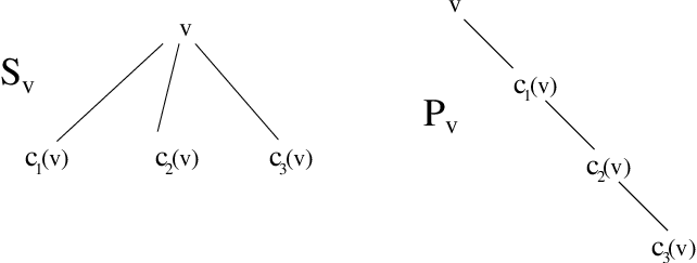
The Procedure $BinExtension$ accepts as input a 4-ary tree $T^{\prime}=(V,E^{\prime})$ rooted at a given vertex $rt\in V$ and transforms it into a binary tree spanning the original set of vertices. If the tree $T^{\prime}$ contains only one node, then the Procedure $BinExtenstion$ leaves the tree intact. Otherwise, for every inner vertex $v\in V$ , the procedure replaces the star $S_{v}=(v,c_{1}(v),\ldots,c_{ch}(v))$ by the path $P_{v}=Path(S_{v})$ . (See Figure 7 for an illustration).

In the next lemma we argue that $T^{\prime\prime}:=BinExtension(T^{\prime})$ is a binary tree.

Lemma 4.17

$T^{\prime\prime}$ is a binary tree such that its root $rt$ has at most one child.

Remark: The notation $c_{i}(v)$ refers to the $i$ th child of $v$ in the tree $T^{\prime}$ that is provided to the Procedure $BinExtension$ as input.

Proof: The vertex $c_{1}(rt)$ is the only child of $rt$ in $T^{\prime}$ . For a vertex $v\in V$ , $v\neq rt$ , let $u$ denote the parent of $v$ in the tree $T^{\prime}$ . Let $i$ be the index such that $v=c_{i}(u)$ . If $i=1$ then $u$ is the parent of $v$ in $T^{\prime\prime}$ . Otherwise, $c_{i-1}(u)$ is the parent of $v$ in $T^{\prime\prime}$ . Moreover, if $i<ch(u)$ then $v$ may have two children in $T^{\prime\prime}$ , specifically, $c_{i+1}(u)$ and $c_{1}(v)$ . If $v$ is a leaf in $T^{\prime}$ then it will have only one child, $c_{i+1}(u)$ . If $i=ch(u)$ then $v$ may have at most one child in $T^{\prime\prime}$ , specifically, $c_{1}(v)$ . In this case if $v$ is a leaf in $T^{\prime}$ then it is a leaf in $T^{\prime\prime}$ as well.

The next two statements imply that both the depth and the weight of $T^{\prime}$ and $T^{\prime\prime}$ are the same, up to a constant factor.

Lemma 4.18

$h(T^{\prime})\leq h(T^{\prime\prime})\leq 4\cdot h(T^{\prime})$ .

Proof: For each vertex $v$ in $T^{\prime}$ , its star subgraph $S_{v}$ is transformed into a path $Path(S_{v})$ of depth $ch(v)$ . Since $T^{\prime}$ is a 4-ary tree, $ch(v)\leq 4$ . Thus the ratio between the depth of $Path(S_{v})$ and the depth of $S_{v}$ is at most $4$ . It follows that for every vertex $v\in V$ , the distance between the root and $v$ in $T^{\prime\prime}$ is at most four times larger than the distance between them in $T^{\prime}$ .

Lemma 4.19

$\omega(T^{\prime\prime})\leq 2\cdot\omega(T^{\prime})$ .

The proof of this lemma is very similar to that of Lemma 4.15, and it is omitted.

We summarize the properties of the reduction from 4-ary to binary trees in the following corollary.

Corollary 4.20

For a 4-ary $\vartheta$ -tree $T^{\prime}=(V,E^{\prime})$ , the Procedure $BinExtension(T^{\prime})$ constructs a binary $\vartheta$ -tree $T^{\prime\prime}$ such that $h(T^{\prime})\leq h(T^{\prime\prime})\leq 4\cdot h(T^{\prime})$ and $\omega(T^{\prime\prime})\leq 2\cdot\omega(T^{\prime})$ .

Corollary 4.16 and Corollary 4.20 imply the following statement.

Lemma 4.21

For a high $\vartheta$ -tree $T=(V,E)$ , the invocation $BinExtension(4Extension(T))$ returns a binary $\vartheta$ -tree $T^{\prime\prime}$ such that $h(T)\leq h(T^{\prime\prime})\leq 8\cdot h(T)$ and $\omega(T^{\prime\prime})\leq 6\cdot\omega(T)$ .

We are now ready to prove the desired lower bound for high $\vartheta$ -trees.

Theorem 4.22

For sufficiently large integers $n$ and $h$ , $h\geq\log n$ , the minimum weight $W(n,h)$ of a general $\vartheta$ -tree that has depth at most $h$ is at least $\Omega(k\cdot n)$ , for some $k$ satisfying $h=\Omega(k\cdot n^{1/k})$ .

Proof: Given an arbitrary $\vartheta$ -tree $T$ of depth $h(T)$ at least $\log n$ , Lemma 4.21 implies the existence of a binary tree $\tilde{T}$ such that $h(\tilde{T})\leq 8\cdot h(T)$ and $\omega(\tilde{T})\leq 6\cdot\omega(T)$ . By Theorem 4.12, the weight $\omega(\tilde{T})$ of $\tilde{T}$ is at least $\Omega(k\cdot n)$ , for some $k$ satisfying $h(\tilde{T})=\Omega(k\cdot n^{1/k})$ . Since $\omega(T)=\Omega(\omega(\tilde{T}))$ and $h(T)=\Omega(h(\tilde{T}))$ , it follows that the weight $\omega(T)$ of $T$ is at least $\Omega(k\cdot n)$ as well, and $k$ satisfies the required relation $h(T)=\Omega(h(\tilde{T}))=\Omega(k\cdot n^{1/k})$ .

Clearly, the lightness of a graph $G$ is at least as large as that of any BFS tree of $G$ , implying the following result.

Corollary 4.23

For sufficiently large integers $n$ and $h$ , $h\geq\log n$ , any spanning subgraph with hop-radius at most $h$ has lightness at least $\Omega(\Psi)$ , for some $\Psi$ satisfying $h=\Omega(\Psi\cdot n^{1/\Psi})$ .

4.2 Lower Bounds for Low Trees

In this section we devise lower bounds for the weight of low $\vartheta$ -trees, that is, trees of depth $h$ at most logarithmic in $n$ .

Our strategy is to show lower bounds for the covering (Section 4.2.1), and then to translate them into lower bounds for the weight (Section 4.2.2).

4.2.1 Lower Bounds for Covering

In this section we prove lower bounds for the covering of trees that have depth $h\leq\frac{1}{5}\cdot\log n$ .

The following lemma shows that for any $\vartheta$ -tree $T$ , the covering of $T$ cannot be much smaller than the maximum degree of a vertex in $T$ .

Lemma 4.24

For a tree $T$ and a vertex $v$ in $T$ , the covering $\chi(T)$ of $T$ is at least $(deg(v)-2)/2$ .

Proof: Consider an edge $(v,u)$ in $T$ . Since every edge adjacent to $v$ is either left or right with respect to $v$ , by the pigeonhole principle either at least $\left\lceil\frac{deg(v)}{2}\right\rceil$ edges are left with respect to $v$ or at least $\left\lceil\frac{deg(v)}{2}\right\rceil$ edges are right with respect to $v$ . Suppose without loss of generality that at least $\left\lceil\frac{deg(v)}{2}\right\rceil$ edges are right with respect to $v$ , and denote by $\mathcal{R}$ the set of edges which are adjacent to $v$ and right with respect to $v$ . Note that all these edges except possibly the edge $(v,v+1)$ cover the vertex $(v+1)$ , and thus the covering of $(v+1)$ is at least

|\mathcal{R}|-1~\geq~\left\lceil\frac{deg(v)}{2}\right\rceil-1\geq\frac{deg(v)-2}{2}.

Though the ultimate goal of this section is to establish a lower bound for the range $h\leq\frac{1}{5}\cdot\log n$ , our argument provides a relationship between covering and depth $h$ in a wider range $h\leq\ln n$ . The next lemma takes care of the simple case of $h$ close to $\ln n$ . The far more complex range of small values of $h$ is analyzed in Lemma 4.26.

Lemma 4.25

For a tree that has depth $h$ and covering $\chi$ , such that $\frac{\ln n}{2}<h\leq{\ln n}$ ,

\chi~>~\frac{1}{e^{2}}\cdot h\cdot n^{1/h}-h.

Proof: We claim that for each $\frac{\ln n}{2}<h\leq{\ln n}$ , the right hand-side is of a negative value. To see this, note that in the range $[1,\ln n]$ , the function $g(h)=\frac{1}{e^{2}}\cdot h\cdot n^{1/h}-h$ is monotone decreasing with $h$ . Thus, $g(h)$ is smaller than $g(\frac{\ln n}{2})=0$ in the range $(\frac{\ln n}{2},\ln n]$ , as required.

Lemma 4.26

For a tree that has depth $h$ and covering $\chi$ , such that $h\leq\frac{\ln n}{2}$ ,

\chi>\frac{1}{10}\cdot h\cdot n^{1/h}-h.

Proof:
The proof is by induction on $h$ , for all values of $n\geq e^{2h}$ .
Base: The statement holds vacuously for $h=0$ . For $h=1$ , the degree of the root is $n-1$ . Hence Lemma 4.24 implies that the covering is at least $\frac{n-3}{2}\geq{\frac{1}{10}\cdot n}-1$ , for any $n\geq e^{2}$ .
Induction Step: We assume the claim for all trees of depth at most $h$ , and prove it for trees of depth $h+1$ . Let $T$ be a tree on $n$ vertices that has depth $h+1$ and covering $\chi$ , such that $h+1\leq\frac{\ln n}{2}$ . If $deg(rt)\geq\sqrt{n}$ , then Lemma 4.24 implies that the covering is at least $\frac{\sqrt{n}-2}{2}$ . It is easy to verify that for $h\geq 1$ and $n\geq e^{2(h+1)}$ ,

\frac{\sqrt{n}-2}{2}\geq\frac{1}{10}\cdot(h+1)\cdot n^{1/(h+1)}-(h+1).

Henceforth, we assume that $deg(rt)<\sqrt{n}$ .

For a child $u$ of $rt$ , denote by $T_{u}$ the subtree of $T$ rooted at $u$ . Such a subtree $T_{u}$ will be called light if $|T_{u}|<e^{h}$ . Denote the set of all light subtrees of $T$ by $\mathcal{L}$ , and define $T^{\prime}$ as the tree obtained from $T$ by omitting all light subtrees from it, namely, $T^{\prime}=T~\setminus~\bigcup_{T_{u}\in\mathcal{L}}T_{u}$ . Observe that the covering $\chi^{\prime}$ of $T^{\prime}$ is at most $\chi$ . Next, we obtain a lower bound on $\chi^{\prime}$ .

Observe that

\left|\bigcup_{T_{u}\in\mathcal{L}}T_{u}\right|~=~\sum_{T_{u}\in\mathcal{L}}|T_{u}|~<~deg(rt)\cdot e^{h}~<~\sqrt{n}\cdot\frac{\sqrt{n}}{e}~=~\frac{n}{e},

implying that

n^{\prime}~=~|T^{\prime}|~=~|T|-\left|\bigcup_{T_{u}\in\mathcal{L}}T_{u}\right|~>~n-n/e.

(17)

Denote the subtrees of $T^{\prime}$ by $T_{1},\ldots,T_{k}$ , where $k\leq deg(rt)$ , and define for each $1\leq i\leq k$ , $n_{i}=|T_{i}|$ , $\chi_{i}=\chi(T_{i})$ , and $h_{i}=depth(T_{i})$ . Fix an index $i$ , $i\in\{1,\ldots,k\}$ . Observe that $n_{i}\geq e^{h}$ , or equivalently, $h\leq\ln n_{i}$ . Since $h_{i}\leq h$ , we have that $h_{i}\leq\ln n_{i}$ . By the induction hypothesis and Lemma 4.25,

\chi_{i}~>~\frac{1}{10}\cdot h_{i}\cdot n_{i}^{1/h_{i}}-h_{i}.

As the function $f(x)=\frac{1}{10}\cdot x\cdot n_{i}^{1/x}-x$ is monotone decreasing in the range $[1,\ln n_{i}]$ , and since $h_{i}\leq h\leq\ln n_{i}$ , it follows that

\chi_{i}~>~\frac{1}{10}\cdot h_{i}\cdot n_{i}^{1/h_{i}}-h_{i}~\geq~\frac{1}{10}\cdot h\cdot n_{i}^{1/h}-h.

Therefore, for each index $i$ , $1\leq i\leq k$ ,

n_{i}~<~\left(\frac{\chi_{i}+h}{\frac{1}{10}\cdot h}\right)^{h}.

(18)

For each $i$ , $1\leq i\leq k$ , choose some vertex $v^{*}_{i}$ in $T_{i}$ with maximum covering, i.e., $\chi_{T_{i}}(v^{*}_{i})=\chi_{i}$ . We assume without loss of generality that

v^{*}_{1}~<~v^{*}_{2}~<~\ldots~<~v^{*}_{k}.

(Note that this order is not necessarily the order of the children $u_{1},u_{2},\ldots,u_{ch(rt)}$ of the root of $T$ . In other words, it may be the case that $v^{*}_{1}<v^{*}_{2}$ but $u_{1}>u_{2}$ .) Let $p$ be the index for which $v^{*}_{p}<rt$ and $v^{*}_{p+1}>rt$ .

Claim 4.27

$\chi^{\prime}\geq\max\{\chi_{1},\chi_{2}+1,\ldots,\chi_{p}+(p-1)\}$ .

Proof: Consider the path in $T^{\prime}$ between $rt$ and $v^{*}_{i}$ , for each $1\leq i\leq p-1$ . For each index $j$ , $i+1\leq j\leq p$ , the vertex $v^{*}_{j}$ must be covered by at least one edge in that path. It follows that $\chi_{T^{\prime}}(v^{*}_{j})\geq\chi_{j}+j-1$ , for each $1\leq j\leq p$ , as required.

A symmetric argument yields the following inequality.

Claim 4.28

$\chi^{\prime}\geq\max\{\chi_{k},\chi_{k-1}+1,\ldots,\chi_{p+1}+(k-p-1)\}$ .

Suppose without loss of generality that ${\displaystyle\sum_{i=1}^{p}n_{i}\geq\sum_{i=p+1}^{k}n_{i}}$ . (The argument is symmetric if this is not the case.) Since $n^{\prime}=|T^{\prime}|=\sum_{i=1}^{k}n_{i},$ it follows that ${\displaystyle\frac{n^{\prime}}{2}~\leq~\sum_{i=1}^{p}n_{i}.}$ By (18), $\sum_{i=1}^{p}n_{i}<\sum_{i=1}^{p}\left(\frac{\chi_{i}+h}{\frac{1}{10}\cdot h}\right)^{h}.$ Notice that for each $1\leq i\leq p$ , $\chi_{i}+i-1~\leq~\chi^{\prime}.$ Consequently,

	$\displaystyle\sum_{i=1}^{p}\left(\frac{\chi_{i}+h}{\frac{1}{10}\cdot h}\right)^{h}$	$\displaystyle\leq$	$\displaystyle\sum_{i=1}^{p}\left(\frac{\chi^{\prime}+h-(i-1)}{\frac{1}{10}\cdot h}\right)^{h}$
		$\displaystyle=$	$\displaystyle 10^{h}\cdot\left(\frac{1}{h}\right)^{h}\cdot\sum_{i=1}^{p}\left(\chi^{\prime}+h-(i-1)\right)^{h}.$

Since $\sum_{i=1}^{p}\left(\chi^{\prime}+h-(i-1)\right)^{h}<\frac{\left(\chi^{\prime}+h+1\right)^{h+1}}{h+1},$ we conclude that

\begin{array}[]{ll}{\displaystyle\frac{n^{\prime}}{2}~<~{10}^{h}\cdot\left(\frac{1}{h}\right)^{h}\cdot\frac{\left(\chi^{\prime}+h+1\right)^{h+1}}{h+1}}\cr\cr{\displaystyle~~~~=~\frac{1}{10}\cdot\left(\frac{h+1}{h}\right)^{h}\cdot\left(\frac{\chi^{\prime}+h+1}{\frac{1}{10}\cdot(h+1)}\right)^{h+1}~\leq~\frac{e}{10}\cdot\left(\frac{\chi^{\prime}+h+1}{\frac{1}{10}\cdot(h+1)}\right)^{h+1}}.\end{array}

(19)

By (17), $n-n/e<n^{\prime}$ , and thus (19) implies that

\frac{n\cdot(1-1/e)}{2}~<~\frac{e}{10}\cdot\left(\frac{\chi^{\prime}+h+1}{\frac{1}{10}\cdot(h+1)}\right)^{h+1},

and consequently, $n<\left(\frac{\chi^{\prime}+h+1}{\frac{1}{10}\cdot(h+1)}\right)^{h+1}.$ It follows that $\chi\geq\chi^{\prime}>\frac{1}{10}\cdot(h+1)\cdot n^{\frac{1}{h+1}}-(h+1),$ as required.

The next corollary follows easily from the above analysis.

Corollary 4.29

For a tree that has depth $h$ and covering $\chi$ , such that $h\leq\frac{1}{5}\cdot\log n$ , it holds that $\chi>\frac{1}{20}\cdot h\cdot n^{1/h}.$

Proof: It is easy to verify that for any $h\leq\frac{1}{5}\cdot\log n$ , it holds that $h<\frac{1}{2}\cdot\left(\frac{1}{10}\cdot h\cdot n^{1/h}\right).$ Hence, the statement follows from Lemma 4.26.

4.2.2 Lower Bounds for Weight

In this section we employ the lower bound for the covering (Corollary 4.29) to show lower bounds for the weight of $\vartheta$ -trees of depth $h<\log n$ . For the range $h\leq\frac{1}{10}\cdot\log n$ , we employ a technique due to Agarwal et al. [3] to translate the lower bound on the covering established in the previous section into the desired lower bound for high trees. (Our lower bound on the covering is, however, significantly stronger than that of [3].) Somewhat surprisingly, our lower bound for the complementary range $\frac{1}{10}\cdot\log n<h<\log n$ relies on our lower bound for the range $h\geq\log n$ (Theorem 4.22).

The following claim establishes a relation between the weight of a tree, and the sum of coverings of its vertices.

Lemma 4.30

For any $\vartheta$ -tree $T$ of depth $h$ , it holds that

\sum_{e\in E(T)}\omega(e)~=~\sum_{v\in V(T)}\chi(v)+n-1.

Proof: For an edge $e\in E(T)$ , let $\varphi(e)$ denote the number of vertices covered by $e$ . Clearly, $\omega(e)=\varphi(e)+1$ . It is easy to verify by double counting that

\sum_{v\in V(T)}\chi(v)~=~\sum_{e\in E(T)}\varphi(e).

Consequently,

\sum_{e\in E(T)}\omega(e)=\sum_{e\in E(T)}(\varphi(e)+1)=\sum_{v\in V(T)}\chi(v)+n-1.

Denote the minimum covering of a $\vartheta$ -tree of depth at most $h$ by $\tilde{\chi}(n,h)$ . Since the sequence $\left(\chi(n,h)\right)_{h=1}^{n-1}$ is monotone non-increasing (by Lemma 3.1), it holds that

\tilde{\chi}(n,h)=\chi(n,h).

(20)

The proof of the following lemma is closely related to the proof of Lemma 2.1 from [3], and is provided for completeness.

Lemma 4.31

For a sufficiently large integer $n$ , and a positive integer $h$ , $h\leq\frac{1}{10}\cdot\log n$ , it holds that

W(n,h)=\Omega(n\cdot h\cdot n^{1/h}).

Proof: Let $T$ be a $\vartheta$ -tree of minimum weight $W(n,h)$ , that has depth at most $h$ , $h\leq\frac{1}{10}\cdot\log n$ , and covering $\chi$ . Denote the root vertex of $T$ by $rt$ . Let $g(n,h)=\frac{1}{20}\cdot h\cdot n^{1/h}$ . By Corollary 4.29 and (20),

\chi>\tilde{\chi}(n,h)\geq g(n,h).

(21)

A vertex $v$ is called heavy if $\chi(v)\geq\frac{1}{6}\cdot g(n,h)$ , and it is called light otherwise. Let $\mathcal{H}$ be the set of heavy vertices in $T$ . Next, we prove that $|\mathcal{H}|\geq n/2$ . Since by Lemma 4.30,

\sum_{e\in E(T)}\omega(e)~\geq~\sum_{v\in V(T)}\chi(v)~\geq~|\mathcal{H}|\cdot\frac{1}{6}\cdot g(n,h),

this would complete the proof of the lemma.

Suppose to the contrary that $|\mathcal{H}|<n/2$ . We need the following definition. A set $B=\{i,i+1,\ldots,j\}$ of consecutive vertices is said to be a block if $B\subseteq\mathcal{H}$ . If $(i-1)\neq B$ and $(j+1)\neq B$ then $B$ is called a maximal block. Decompose $\mathcal{H}$ into a set of (disjoint) maximal blocks $\mathcal{B}=\{B_{1},B_{2},\ldots,B_{k}\}$ . By contracting the induced subgraph of each $B_{i}$ into a single node $w_{i}$ , for $1\leq i\leq k$ , we obtain a new graph $G^{\prime}=(V^{\prime},E^{\prime})$ . Observe that $G^{\prime}$ is not necessarily a tree and may contain multiple edges connecting the same pair of vertices. For each pair of vertices $u$ and $v$ in $V^{\prime}$ , omit all edges except for the lightest one that connect $u$ and $v$ in $T^{\prime}$ . If $rt\in w_{i}$ , for some index $i\in[1,k]$ , then designate $w_{i}$ as the new root vertex $rt$ . Let $T^{\prime}=(V^{\prime},E^{\prime\prime})$ be the BFS tree of $G^{\prime}$ rooted at $rt$ . Clearly, $n^{\prime}=|V^{\prime}|\geq|V\setminus\mathcal{H}|>n/2$ , and $h(T^{\prime})\leq h(T)=h$ . Let $v_{1},v_{2},\ldots,v_{n^{\prime}}$ be the vertices of $T^{\prime}$ in an increasing order. Transform $T^{\prime}$ into a spanning tree $\tilde{T}$ of $\vartheta_{n^{\prime}}$ by mapping each $v_{i}$ to the point $i$ on the $x$ -axis, for $i=1,2,\ldots,n^{\prime}$ .

Claim 4.32

$\chi(\tilde{T})\leq\frac{1}{3}\cdot g(n,h)+1$ .

Proof: First, observe that all light vertices in $T$ remain light in $\tilde{T}$ . For a contracted heavy vertex $w_{i}$ , we argue that $\chi(w_{i})\leq\chi(w_{i}^{-})+\chi(w_{i}^{+})+1$ , where $w_{i}^{-}$ (respectively, $w_{i}^{+}$ ) is the vertex to the immediate left (resp., right) of $w_{i}$ . To see this, note that for each edge $e\neq(w_{i}^{+},w_{i}^{-})$ that covers $w_{i}$ , $e$ covers either $w_{i}^{-}$ or $w_{i}^{+}$ . Since both vertices $w_{i}^{+}$ and $w_{i}^{-}$ are light, it follows that $\chi(w_{i})\leq 2\cdot\left(\frac{1}{6}\cdot g(n,h)\right)+1$ , and we are done.

Observe that for $n\geq 4$ , we have that $\frac{1}{10}\cdot\log n\leq\frac{1}{5}\cdot\log(n/2).$ Since $h\leq\frac{1}{10}\cdot\log n$ , and $n^{\prime}>n/2$ , it follows that $h\leq\frac{1}{5}\cdot\log n^{\prime}$ . Hence by Corollary 4.29 and (21),

	$\displaystyle\chi(\tilde{T})$	$\displaystyle\geq$	$\displaystyle\tilde{\chi}(n^{\prime},h)~\geq~g(n^{\prime},h)~=~\frac{1}{20}\cdot h\cdot{n^{\prime}}^{\frac{1}{h}}$
		$\displaystyle>$	$\displaystyle\frac{1}{20}\cdot h\cdot{(n/2)}^{\frac{1}{h}}~=~\left(\frac{1}{2}\right)^{\frac{1}{h}}\cdot g(n,h).$

However, for sufficiently large $n$ ,

\left(\frac{1}{2}\right)^{\frac{1}{h}}\cdot g(n,h)>\frac{1}{3}\cdot g(n,h)+1,

contradicting Claim 4.32.

Lemma 4.33

For a sufficiently large integer $n$ , and a positive integer $h$ , $\frac{1}{10}\cdot\log n\leq h<\log n$ , it holds that $W(n,h)=\Omega(n\cdot h\cdot n^{1/h}).$

Proof: By Theorem 4.22, the minimum weight $W(n,\log n)$ of a $\vartheta_{n}$ -tree that has depth $h$ , $h\leq\log n$ , is at least $\Omega(k\cdot n)$ , for some $k$ satisfying $\log n=\Omega(k\cdot n^{1/k})$ . It follows that $W(n,\log n)=\Omega(\log n\cdot n)$ .
Since by Lemma 3.2, the sequence $\left(W(n,h)\right)|_{h=1}^{n-1}$ is monotone non increasing, it holds that for $h\in[\frac{1}{10}\cdot\log n,\log n]$ ,

W(n,h)=\Omega(\log n\cdot n)=\Omega(n\cdot h\cdot n^{1/h}).

Lemmas 4.30 and 4.33 imply the following lower bound for $h<\log n$ .

Corollary 4.34

For a sufficiently large integer $n$ , and a positive integer $h$ , $h<\log n$ , it holds that $W(n,h)=\Omega(n\cdot h\cdot n^{1/h}).$

Clearly, the lightness of a graph $G$ is at least as large as that of any BFS tree of $G$ , implying the following result.

Theorem 4.35

For a sufficiently large integer $n$ and a positive integer $h$ , $h<\log n$ , any spanning subgraph with hop-radius at most $h$ has lightness at least $\Psi=\Omega(h\cdot n^{1/h})$ .

5 Euclidean Spanners

The following theorem is a direct corollary of Theorem 4.22 and Corollary 4.34. It implies that no construction that provides Euclidean spanner with hop-diameter $O(\log n)$ and lightness $o(\log n)$ , or vice versa, is possible. This settles the open problem of [6, 3].

Theorem 5.1

For a sufficiently large integer $n$ , any spanning subgraph of $\vartheta$ with hop-diameter at most $O(\log n)$ has lightness at least $\Omega(\log n)$ , and vice versa.

Proof: First, we show that any $\vartheta$ -tree that has depth at most $O(\log n)$ has lightness at least $\Omega(\log n)$ . If the depth $h$ is at least $\log n$ , Theorem 4.22 implies that the lightness is at least $\Omega(k)$ , for some $k$ satisfying $h=\Omega(k\cdot n^{1/k})$ . Observe that for $h=O(\log n)$ , any $k$ that satisfies $h=\Omega(k\cdot n^{1/k})$ is at least $\Omega(\log n)$ , as required. By the monotonicity (Lemma 3.2), the lower bound of $\Omega(\log n)$ applies for all smaller values of $h$ .

Consider a spanning subgraph $G$ of $\vartheta$ that has hop-diameter $\Lambda=O(\log n)$ . Consider a BFS tree $T$ rooted at some vertex $rt$ . Obviously, $h(T,rt)\leq\Lambda=O(\log n)$ , and thus $\omega(T)=\Omega(\log n)\cdot\omega(MST(\vartheta))=\Omega(n\log n)$ . Since $\omega(G)\geq\omega(T)$ , it follows that the lightness of $G$ is $\Omega(\log n)$ as well.

Next, we argue that any $\vartheta$ -tree that has lightness at most $O(\log n)$ has depth at least $\Omega(\log n)$ . Indeed, by Corollary 4.34, any $\vartheta$ -tree of depth $h=o(\log n)$ has lightness at least $\Omega(h\cdot n^{1/h})=\omega(\log n)$ . Moreover, if a spanning subgraph $G$ of $\vartheta$ has lightness $\Psi(G)=O(\log n)$ , then its BFS tree $T$ satisfies $\Psi(T)=O(\log n)$ as well. Therefore, $h(T,rt)=\Omega(\log n)$ , and thus $\Lambda(G)\geq h(T,rt)=\Omega(\log n)$ .

6 Upper Bounds

In this section we devise an upper bound for the tradeoff between various parameters of binary LLTs. This upper bound is tight up to constant factors in the entire range of parameters.

Consider a general $n$ -point metric space $M$ . Let $T^{*}$ be an MST for $M$ , and $D$ be an in-order traversal of $T^{*}$ , starting at an arbitrary vertex $v$ . For every vertex $x$ , remove from $D$ all occurrences of $x$ except for the first one. It is well-known ([25], ch. 36) that this way we obtain a Hamiltonian path $L=L(T)$ of $M$ of total weight

\omega(L)=\sum_{e\in L}\omega(e)\leq 2\cdot\omega(MST(M)).

Let $(v_{1},v_{2},\ldots,v_{n})=L$ be the order in which the points of $M$ appear in $L$ . Consider an edge $e^{\prime}=(v_{i},v_{j})$ connecting two arbitrary points in $M$ , and an edge $e=(v_{q},v_{q+1})\in E(L)$ , $q\in[n-1].$ The edge $e^{\prime}$ is said to cover $e$ with respect to $L$ if $i\leq q<q+1\leq j$ . When $L$ is clear from the context, we write that $e^{\prime}$ covers $e$ .

For a spanning tree $T$ of $M$ , the number of edges $e^{\prime}\in E(T)$ that cover an edge $e$ of $E(L)$ is called the load of $e$ by $T$ and it is denoted $\xi(e)=\xi_{T}(e)$ . The load of the tree $T$ , $\xi(T)$ , is the maximum load of an edge $e\in E(L)$ by $T$ , i.e.,

\xi(T)=\max\{\xi_{T}(e)~|~e\in E(L)\}.

Observe that

\omega(T)~\leq~\sum_{e\in L(T)}\xi_{T}(e)\cdot\omega(e)~\leq~\xi(T)\cdot w(L),

and so,

\xi(T)\geq\frac{\omega(T)}{\omega(L)}\geq\frac{1}{2}\cdot\Psi(T).

(22)

(See Figure 8 for an illustration.)

In the sequel we provide an upper bound for the load $\xi(T)$ of a tree $T$ , which yields the same upper bound for the lightness $\Psi(T)$ of $T$ , up to a factor of 2. Since the weight of a tree $T$ does not affect its load, we may assume without loss of generality that $v_{i}$ is located in the point $i$ on the $x$ -axis.

Lemma 6.1

Suppose there exists a $\vartheta$ -tree $T$ with load $\xi(T)$ and depth $h$ . Then there exists a spanning tree $T^{\prime}$ for $M$ with the same load (with respect to $L(T)$ ) and depth.

Proof: The edge set $E^{\prime}$ of the tree $T^{\prime}$ is defined by $E^{\prime}=\{(v_{i},v_{j})|(i,j)\in T\}$ . It is easy to verify that its depth and load are equal to those of $T$ .

Consequently, the problem of providing upper bounds for general metric spaces reduces to the problem of providing upper bounds for $\vartheta$ .

6.1 Upper Bounds for High Trees

In this section we devise a construction of $\vartheta_{n}$ -trees with depth $h\geq\log n$ . This construction exhibits tight up to constant factors tradeoff between load and depth, when the tree depth is at least logarithmic in the number of vertices. In addition, the constructed trees are binary, and so their maximum degree is optimal.

We start with defining a certain composition of binary trees. Let $n^{\prime}$ and $n^{\prime\prime}$ be two positive integers, $n=n^{\prime}+n^{\prime\prime}$ . Let $\vartheta^{\prime}$ , $\vartheta^{\prime\prime}$ , and $\vartheta$ be the $n^{\prime}$ -, $n^{\prime\prime}$ - and $n$ -point metric spaces $\vartheta_{n^{\prime}}$ , $\vartheta_{n^{\prime\prime}}$ , and $\vartheta_{n}$ , respectively. Also, let $\{v^{\prime}_{1},v^{\prime}_{2},\ldots,v^{\prime}_{n^{\prime}}\}$ , $\{v^{\prime\prime}_{1},v^{\prime\prime}_{2},\ldots,v^{\prime\prime}_{n^{\prime\prime}}\}$ , and $\{\tilde{v}_{1},\tilde{v}_{2},\ldots,\tilde{v}_{n}\}$ denote the set of points of $\vartheta^{\prime}$ , $\vartheta^{\prime\prime}$ , and $\vartheta$ , respectively. Consider spanning trees $T^{\prime}$ and $T^{\prime\prime}$ for $\vartheta^{\prime}$ and $\vartheta^{\prime\prime}$ , respectively. Let $v^{\prime}=v^{\prime}_{i}$ be a vertex of $T^{\prime}$ . Consider a tree $\tilde{T}$ that spans the vertex set $\{\tilde{v}_{1},\tilde{v}_{2},\ldots,\tilde{v}_{n^{\prime}+n^{\prime\prime}}\}$ formed out of the trees $T^{\prime}$ and $T^{\prime\prime}$ in the following way. The root $rt^{\prime\prime}$ of $T^{\prime\prime}$ is added as a right child of $v^{\prime}$ in $\tilde{T}$ . The vertices $v^{\prime}_{1},v^{\prime}_{2},\ldots,v^{\prime}_{i}=v^{\prime}$ of $T^{\prime}$ retain their indices, and are translated into vertices $\tilde{v}_{1},\tilde{v}_{2},\ldots,\tilde{v}_{i}$ in $\tilde{T}$ . The vertices $v^{\prime\prime}_{1},v^{\prime\prime}_{2},\ldots,v^{\prime\prime}_{n^{\prime\prime}}$ of $T^{\prime\prime}$ get the index $i$ of $v^{\prime}_{i}$ , added to their indices, and are translated into vertices $\tilde{v}_{i+1},\tilde{v}_{i+2},\ldots,\tilde{v}_{i+n^{\prime\prime}}$ in $\tilde{T}$ . Finally, the vertices $v^{\prime}_{i+1},v^{\prime}_{i+2},\ldots,v^{\prime}_{n^{\prime}}$ of $T^{\prime}$ get the number $n^{\prime\prime}$ of vertices of $T^{\prime\prime}$ added to their indices, and are translated into vertices $\tilde{v}_{i+1+n^{\prime\prime}},\tilde{v}_{i+2+n^{\prime\prime}},\ldots,\tilde{v}_{n^{\prime}+n^{\prime\prime}}$ . We say that the tree $\tilde{T}$ is composed by adding $T^{\prime\prime}$ as a right subtree to the vertex $v$ in $T^{\prime}$ . Adding a left subtree $T^{\prime\prime}$ to a vertex $v$ in $T^{\prime\prime}$ is defined analogously.

Consider a family of binary $\vartheta$ -trees $T(\xi,h)$ with $n=N(\xi,h)$ vertices, load $\xi$ and depth $h$ , $h\geq\xi-1$ , $\xi\geq 1$ . These trees are all rooted at the point $1$ . For $\xi=1$ , and $h=0$ , the tree $T(1,0)$ is a singleton vertex, and so $N(1,0)=1$ . For convenience, we define the load of $T(1,0)$ to be 1. For $\xi=1$ and $h\geq 1$ , the tree $T(1,h)$ is the path $P_{h+1}=(v_{1},v_{2},\ldots,v_{h+1})$ . The depth of $T(1,h)$ is equal to $h$ , and its load is 1. Hence $N(1,h)=h+1$ .

For $\xi\geq 2$ and $h\geq\xi-1$ , the tree $T(\xi,h)$ is constructed as follows. Let $T^{\prime}=P_{h+1}$ be the path $(v_{1},v_{2},\ldots,v_{h+1})$ , and for each index $i$ , $i\in[h]$ , define for technical convenience $v^{\prime}_{i}=v_{i}$ . For each index $i$ , $i\in[h]$ , let $T^{\prime\prime}_{i}$ be the tree $T(\xi^{\prime\prime}_{i},h^{\prime\prime}_{i})$ , with $\xi^{\prime\prime}_{i}=\min\{\xi-1,h-i+1\}$ , $h^{\prime\prime}_{i}=h-i$ . Observe that for each $i\in[h]$ , $h^{\prime\prime}_{i}\geq\xi^{\prime\prime}_{i}-1$ , and thus the tree $T^{\prime\prime}_{i}$ is well-defined. For every $i\in[h]$ , we add the tree $T^{\prime\prime}_{i}$ as a right subtree of $v^{\prime}_{i}$ in $T^{\prime}$ . (See Figure 9 for an illustration.)

Lemma 6.2

The depth of the resulting tree $T(\xi,h)$ with respect to the vertex $v^{\prime}_{1}$ is $h$ , and its load is $\xi$ .

Proof: The proof is by induction on $\xi$ , for all values of $h\geq\xi-1$ .
Base $(\xi=1)$ : The tree $T(1,h)$ has load 1 and depth $h$ , as required.
Induction Step: We assume the correctness of the statement for all smaller values of $\xi$ , and prove it for $\xi$ . First, the vertex $v^{\prime}_{h+1}$ is connected to the root $v^{\prime}_{1}$ via the path $P_{h+1}$ , and thus the depth $h(T(\xi,h))$ of $T(\xi,h)$ is at least the length of this path, that is, $h$ . Consider a vertex $u\in V(T^{\prime\prime}_{i})$ , for some $i\in[h]$ . The path $P_{u}$ connecting $v^{\prime}_{1}$ and $u$ in $T(\xi,h)$ starts with a subpath $(v^{\prime}_{1},v^{\prime}_{2},\ldots,v^{\prime}_{i},rt(T^{\prime\prime}_{i}))$ , and continues with the unique path $P^{\prime\prime}_{u}$ connecting between the root of $T^{\prime\prime}_{i}$ and the vertex $u$ in the tree $T^{\prime\prime}_{i}$ . The length of the latter path is no greater than the depth of $T^{\prime\prime}_{i}$ , which, by the induction hypothesis, is equal to $h-i$ . Hence $|P_{u}|=i+|P^{\prime\prime}_{u}|\leq h$ . Hence $h(T(\xi,h))=h$ .

To analyze the load $\xi(T(\xi,h))$ of the tree $T(\xi,h)$ , consider some edge $e=(v_{q},v_{q+1})$ of the path $P_{n}$ , where $n$ is the number of vertices in $T(\xi,h)$ . The path $T^{\prime}$ contributes at most one unit to the load of $e$ . In addition, there exists at most one index $i$ , $i\in[h]$ , such that the tree $T^{\prime\prime}_{i}$ covers the edge $e$ . By induction, the load $\xi(T^{\prime\prime}_{i})$ is equal to $\min\{\xi-1,h-i+1\}$ . Consequently, the load of $e$ is

	$\displaystyle\xi_{T(\xi,h)}(e)$	$\displaystyle\leq$	$\displaystyle\max\{\min\{\xi-1,h-i+1\}+1~\|~i\in[h]\}$
		$\displaystyle=$	$\displaystyle\min\{\xi-1,h\}+1~=~\xi.$

Finally, we analyze the number of vertices $N(\xi,h)$ in the tree $T(\xi,h)$ . By construction,

N(\xi,h)=h+1+\sum_{i=1}^{h}N(\min\{\xi-1,h-i+1\},h-i).

Lemma 6.3

For $h\geq\xi-1$ , $N(\xi,h)\geq{h\choose\xi}$ .

Proof: The proof is by induction on $\xi$ .
Base: For $\xi=1$ , $N(1,h)=h+1\geq{h\choose 1}$ , as required.
Step: For $\xi\geq 2$ , and $i\leq h-\xi+1$ , $\min\{\xi-1,h-i+1\}=\xi-1$ . Hence

	$\displaystyle N(\xi,h)$	$\displaystyle\geq$	$\displaystyle h+1+\sum_{i=1}^{h}N(\min\{\xi-1,h-i+1\},h-i)$
		$\displaystyle\geq$	$\displaystyle\sum_{i=1}^{h-\xi+1}N(\min\{\xi-1,h-i+1\},h-i)~=~\sum_{i=1}^{h-\xi+1}N(\xi-1,h-i).$

Observe that for each index $i$ , $i\in[h-\xi+1]$ , $h-i\geq\xi-1$ . Hence, by the induction hypothesis and Fact A.1, the latter sum is at least

\sum_{i=1}^{h-\xi+1}{h-i\choose\xi-1}~=~{h\choose\xi}.

The following theorem summarizes the properties of the trees $T(\xi,h)$ .

Theorem 6.4

For a sufficiently large $n$ , and $h$ , $h\geq 2\log n$ , there exists a binary $\vartheta_{n}$ -tree that has depth at most $h$ and load at most $\xi$ , where $\xi$ satisfies ( $h=O(n^{1/\xi}\cdot\xi)$ and $\xi=O(\log n)$ ).

Proof: First, note that for $h$ in this range, ${h\choose\log n}>n$ . By Lemma 6.3, for any pair of positive integers $h$ and $\xi$ such that $\xi-1\leq h$ , it holds that $N(\xi,h)\geq{h\choose\xi}$ . Further, observe that $N(\xi,h)$ is monotone increasing with both $\xi$ and $h$ , in the entire range $0\leq\xi-1\leq h$ . It follows that for $h\geq 2\log n$ , there exists a positive integer $\xi$ , $\xi\leq h$ , such that $N(\xi,h-1)\leq n<N(\xi,h)$ .

Consider the binary tree obtained from the tree $T(\xi,h)$ by removing $N(\xi,h)-n$ leaves from it, one after another. Clearly, the resulting tree has depth at most $h$ , load at most $\xi$ , and its number of vertices is equal to $n$ . Observe that

n~\geq~N(\xi,h-1)~\geq~{h-1\choose\xi}~\geq~\left(\frac{h-1}{\xi}\right)^{\xi},

implying that

h~\leq~n^{1/\xi}\cdot\xi+1~=~O(n^{1/\xi}\cdot\xi).

The next corollary employs Theorem 6.4 to deduce an analogous result for general metric spaces.

Corollary 6.5

For sufficiently large $n$ and $h$ , $h\geq 2\log n$ , there exists a binary spanning tree of $M$ that has depth at most $h$ and lightness at most $2\cdot\Psi$ , where $\Psi$ satisfies ( $h=O(n^{1/\Psi}\cdot\Psi)$ and $\Psi=O(\log n)$ ). Moreover, this binary tree can be constructed in time $O(n^{2})$ .

Remark: If $M$ is an Euclidean 2-dimensional metric space, the running time can be further improved to $O(n\cdot\log n)$ . This is because the running time of this construction is dominated by the running time of the subroutine for constructing MST, and an MST of an Euclidean 2-dimensional metric space can be constructed in $O(n\cdot\log n)$ time [31]. By the same considerations, for Euclidean 3-dimensional spaces our algorithm can be implemented in a randomized time of $O(n\cdot\log^{4/3}n)$ , and more generally, for dimension $d=3,4,\ldots$ it can be implemented in deterministic time $O(n^{2-\frac{2}{\lceil d/2\rceil+1}+\epsilon})$ , for an arbitrarily small $\epsilon>0$ (cf. [31], page 5). Even better time bounds can be provided if one uses a $(1+\epsilon)$ -approximation MST instead of the exact MST for Euclidean metric spaces (cf. [31], page 6).

Proof: By Theorem 6.4 and Lemma 6.1, for a sufficiently large $n$ , and $h$ , $h\geq 2\log n$ , there exists a binary spanning tree $T$ of $M$ that has depth at most $h$ and load at most $\Psi$ , where $\Psi$ satisfies $h=O(n^{1/\Psi}\cdot\Psi)$ . By (22), the lightness $\Psi(T)$ is at most $2\Psi$ . Note that since the complete graph $G(M)$ induced by the metric $M$ contains at most $O(n^{2})$ edges, its MST can be computed within $O(n^{2})$ time (cf. [25], chapter 23). The in-order traversal, and the construction of the tree $T(\xi,h)$ can be performed in $O(n)$ time in the straight-forward way. Hence the overall running time of the algorithm for computing an LLT with the specified properties is $O(n^{2})$ .

Finally, we present a simple construction for the range $\log n\leq h<2\log n$ . Consider a full³³ 3 Strictly speaking, this tree is full when $n=2^{k}-1$ , for integer $k\geq 1$ . However, for simplicity of presentation, we call it “full” for other values of $n$ as well. balanced binary spanning tree $T_{n}$ of $\{1,2,\ldots,n\}$ . The root of $T_{n}$ is $\lceil n/2\rceil$ . Its left (respectively, right) subtree is the full balanced binary tree constructed recursively from the vertex set $\{1,\ldots,\lceil n/2\rceil-1\}$ (resp., $\{\lceil n/2\rceil+1,\ldots,n\}$ ). (See Figure 10 for an illustration.)

Lemma 6.6

Both the depth and the load of $T_{n}$ are no greater than $\log n$ .

Proof: The proof is by induction on $n$ . The base is trivial.
Induction Step: We assume the correctness of the claim for all smaller values of $n$ , and prove it for $n$ . By the induction hypothesis, the depth of both the left and the right subtrees of the root $\lceil n/2\rceil$ is at most $\log(n/2)$ , implying that the depth $h(T_{n})$ of $T_{n}$ is at most $\log(n/2)+1=\log n$ , as required.

To analyze the load $\xi(T_{n})$ of the tree $T_{n}$ , consider some edge $e=(v_{q},v_{q+1})$ of the path $L_{n}$ . The two edges connecting $rt$ to its children contribute at most one unit to the load of $e$ . In addition, at most one among the subtrees of the root $\lceil n/2\rceil$ covers the edge $e$ . By induction, both of these subtrees has load no greater than $\log(n/2)$ . Consequently, the load of $e$ is at most $\log(n/2)+1=\log n$ .

Theorem 6.7

For a sufficiently large $n$ , and $h$ , $\log n\leq h<2\log n$ , there exists a binary $\vartheta_{n}$ -tree that has depth at most $h$ and load at most $\xi$ , where $\xi$ satisfies $h=O(n^{1/\xi}\cdot\xi)$ . (In this case $\xi=O(\log n)$ .)

Proof: By Lemma 6.6, for a sufficiently large $n$ , and $h$ , $\log n\leq h<2\log n$ , the binary tree $T_{n}$ has depth at most $h$ , and load at most $\xi=\log n$ , where $h=O(n^{1/\xi}\cdot\xi)$ .

The next corollary employs Theorem 6.7 to deduce an analogous result for general metrics.

Corollary 6.8

For sufficiently large $n$ and $h$ , $\log n\leq h<2\log n$ , there exists a binary spanning tree of $M$ that has depth at most $h$ and lightness at most $2\cdot\Psi$ , where $\Psi$ satisfies $h=O(n^{1/\Psi}\cdot\Psi)$ .

Proof: By Theorem 6.7 and Lemma 6.1, for a sufficiently large $n$ , and $h$ , $\log n\leq h<2\log n$ , there exists a binary spanning tree of $M$ that has depth at most $h$ and load at most $\Psi$ , where $\Psi$ satisfies $h=O(n^{1/\Psi}\cdot\Psi)$ . By (22), the lightness is at most twice the load, and we are done.

Remark: By the same considerations as those of Corollary 6.5, this construction can be implemented within time $O(n^{2})$ in general metric spaces, and in time $O(n\cdot\mbox{polylog}(n))$ in Euclidean low-dimensional ones.

6.2 Upper Bounds for Low Trees

In this section we devise a construction of $\vartheta_{n}$ -trees with depth in the range of $h<\log n$ . Like the construction in Section 6.1, this construction provides a tight up to constant factors upper bound for the tradeoff between weight and depth. In addition, the maximum degree of the constructed trees is optimal as well. (It is $\lceil n^{1/h}\rceil$ ).

We devise a family of $d$ -regular trees $\tilde{T}(d,h)$ with ${\displaystyle\tilde{N}(d,h)=\sum_{i=0}^{h}d^{i}}$ vertices, load $\xi\leq d\cdot h$ , depth $h$ , and $d\geq 2$ . Since $d\geq 2$ , it holds that $\tilde{N}(d,h)=\frac{d^{h+1}-1}{d-1}$ . The family $\tilde{T}(d,h)$ is constructed recursively as follows. For $h=0$ , the tree $T_{0}=\tilde{T}(d,0)$ is a singleton vertex, and so $\tilde{N}(d,0)=1$ . For $h\geq 1$ , the tree $\tilde{T}(d,h)$ is constructed as follows. For each $i\in[d]$ , let $T_{i}$ be a copy of $\tilde{T}(d,h-1)$ , and let $T_{0}=\tilde{T}(d,0)$ . For every $i\in[\lceil d/2\rceil]$ , we add the tree $T_{i}$ as a left subtree of the root vertex $rt$ of $T_{0}$ , and for each $i\in[\lceil d/2\rceil+1,d]$ , we add the tree $T_{i}$ as a right subtree of $rt$ .

Lemma 6.9

The depth of the resulting tree $\tilde{T}(d,h)$ with respect to the vertex $rt$ is $h$ , its load $\xi$ is at most $d\cdot h$ , and its size is equal to ${\displaystyle\sum_{i=0}^{h}d^{i}}$ .

Proof: The proof is by induction on $h$ . The base $h=0$ is trivial.
Induction Step: We assume the correctness of the claim for all smaller values of $h$ , and prove it for $h$ . By construction, the root $rt$ has $d$ children, each being the root of a tree $\tilde{T}(d,h-1)$ . By the induction hypothesis, $\tilde{T}(d,h-1)$ has depth $h$ and size ${\displaystyle\sum_{i=0}^{h-1}d^{i}}$ . Obviously, the depth of $\tilde{T}(d,h)$ is equal to $h$ . To estimate the size $\tilde{N}(d,h)$ of $\tilde{T}(d,h)$ , note that

\tilde{N}(d,h)=1+d\cdot\tilde{N}(d,h-1)=1+d\cdot\left(\sum_{i=0}^{h-1}d^{i}\right)=\sum_{i=0}^{h}d^{i}.

To analyze the load $\xi(\tilde{T}(d,h))$ of the tree $\tilde{T}(d,h)$ , consider some edge $e=(v_{q},v_{q+1})$ of the path $L_{\tilde{n}}$ , where $\tilde{n}$ is the number of vertices in $\tilde{T}(d,h)$ . The $d$ edges connecting $rt$ to its children contribute altogether at most $d$ units to the load of $e$ . In addition, there exists at most one index $i$ , $i\in[h]$ , such that the tree $T_{i}$ covers the edge $e$ . By the induction hypothesis, the load $\xi(T_{i})$ of $T_{i}$ is no greater than $d(h-1)$ . Consequently, the load of $e$ is at most $d(h-1)+d=d\cdot h$ , and we are done.

Theorem 6.10

For any positive integers $n$ and $h$ , $h<\log n$ , there exists an $\left\lceil n^{1/h}\right\rceil$ -ary $\vartheta_{n}$ -tree that has depth at most $h$ , and load at most $\left\lceil n^{1/h}\right\rceil\cdot h$ .

The case $h=0$ is trivial.
For $h>0$ , observe that $\tilde{N}(d,h)$ is monotone increasing with both $d$ and $h$ . Given a pair of positive integers $n$ and $h$ , $1\leq h<\log n$ , let $d$ be the positive integer that satisfies $\tilde{N}(d-1,h)\leq n<\tilde{N}(d,h)$ .

Consider the $d$ -ary tree obtained from $\tilde{T}(d,h)$ by removing $\tilde{N}(d,h)-n$ leaves from it, one after another. Clearly, the depth, the load, and the maximum degree of the resulting tree are no greater than those of the original tree $\tilde{T}(d,h)$ . Moreover, the size of the resulting tree is precisely $n$ . Observe that

n~\geq~\tilde{N}(d-1,h)~=~\sum_{i=0}^{h}(d-1)^{i}~>~(d-1)^{h},

implying that $d<n^{1/h}+1$ . It follows that $d\leq\left\lceil n^{1/h}\right\rceil$ . Thus by Lemma 6.9, the resulting tree is a spanning $\left\lceil n^{1/h}\right\rceil$ -ary tree of size $n$ that has depth at most $h$ , and load at most $\left\lceil n^{1/h}\right\rceil\cdot h$ , and we are done.

The next corollary is an extension of Theorem 6.10 to general metric spaces.

Corollary 6.11

For a sufficiently large $n$ , and $h$ , $h<\log n$ , there exists a spanning $\left\lceil n^{1/h}\right\rceil$ -ary tree of $M$ that has depth at most $h$ , and lightness at most $O(n^{1/h}\cdot h)$ .

Proof: By Theorem 6.10 and Lemma 6.1, for a sufficiently large $n$ , and $h$ , $h<\log n$ , there exists a spanning $\left\lceil n^{1/h}\right\rceil$ -ary tree of $M$ that has depth at most $h$ and load at most $\left\lceil n^{1/h}\right\rceil\cdot h$ . By (22), the lightness is at most twice the load, and we are done.

Remark: By the same considerations as in Section 6.1, this construction can be implemented within time $O(n^{2})$ in general metric spaces, and in time $O(n\cdot\mbox{polylog}(n))$ in Euclidean low-dimensional ones.

Corollaries 6.5, 6.11 and 6.8 imply the following theorem.

Theorem 6.12

For any sufficiently large integer $n$ and positive integer $h$ , and $n$ -point metric space $M$ , there exists a spanning tree of $M$ of depth at most $h$ and lightness at most $O(\Psi)$ , that satisfies the following relationship. If $h\geq\log n$ then ( $h=O(\Psi\cdot n^{1/\Psi})$ and $\Psi=O(\log n)$ ). In the complementary range $h<\log n$ , $\Psi=O(h\cdot n^{1/h})$ .
Moreover, this spanning tree is a binary one for $h\geq\log n$ , and it has the optimal maximum degree $\left\lceil n^{1/h}\right\rceil$ , for $h<\log n$ .

7 Shallow-Low-Light-Trees

In this section we extend our construction of low-light-trees and construct shallow-low-light trees. Our argument in this section is closely related to that of Awerbuch et al. [10].

Consider a spanning tree $T=(V,E)$ of an $n$ -point metric space $M$ , rooted at a root vertex $rt$ , having depth $h(T)$ and weight $\omega(T)$ . We construct a spanning tree $S(T)$ of $M$ that has the same depth and weight, up to constant factors, and that also approximates the distances between the root vertex $rt$ and all other vertices in $V$ . (Thus, for a low-light tree $T$ , $S(T)$ is a shallow-low-light tree.)

Let $L=(v_{1},v_{2},\ldots,v_{n})$ be the sequence of vertices of $T$ , ordered according to an in-order traversal of $T$ , starting at $rt$ . Fix a parameter $\theta$ to be a positive real number. The value of $\theta$ determines the values of other parameters of the constructed tree.
We start with identifying a set of “break-points” $\mathcal{B}=\{B_{1},B_{2},\ldots,B_{k}\}$ , $\mathcal{B}\subseteq V$ . The break-point $B_{1}$ is the vertex $v_{1}$ . The break-point $B_{i}$ is the first vertex in $L$ after $B_{i-1}$ such that

dist_{T}(B_{i-1},B_{i})>\theta\cdot dist_{M}(rt,B_{i}).

Let $\mathcal{S}$ be the set of edges connecting the break-points with $rt$ in $M$ , namely, $\mathcal{S}=\{(rt,B_{i})|B_{i}\in\mathcal{B}\}$ . Let $\tilde{G}=(V,E\cup\mathcal{S})$ be the graph obtained from $T$ by adding to it all edges in $\mathcal{S}$ .
Finally, we define $S(T)$ to be the shortest-path-tree (henceforth, SPT) tree of $\tilde{G}$ rooted at $rt$ .

The following claim implies that the sum of distances in $T$ , taken over all pairs of consecutive break-points, is not too large.

Claim 7.1

$\sum_{B_{i}\in\mathcal{B}}dist_{T}(B_{i-1},B_{i})~\leq~2\cdot\omega(T).$

Proof: First, observe that any in-order traversal of $T$ visits each edge exactly twice. Hence, since the vertices in $L$ are ordered according to an in-order traversal of $T$ , we have that $\sum_{i=2}^{n}dist_{T}(v_{i-1},v_{i})~\leq~2\cdot\omega(T).$

Clearly, for any pair of vertices $v_{i}$ and $v_{j}$ , $1\leq i\leq j\leq n$ , it holds that $dist_{T}(v_{j},v_{k})\leq\sum_{i=j+1}^{k}dist_{T}(v_{i-1},v_{i})$ . It follows that $\sum_{i=2}^{k}dist_{T}(B_{i-1},B_{i})\leq\sum_{i=2}^{n}dist_{T}(v_{i-1},v_{i})$ , and we are done.

The following three lemmas imply that the depth, the weight, and the weighted diameter of the constructed tree $S(T)$ are not much greater than those of the original tree $T$ . In fact, if we set $\theta$ to be a small constant, the three parameters do not increase by more than a small constant factor. Moreover, not only the weighted diameter does not grow too much, but, in fact, all distances between the root vertex $rt$ and other vertices in the graph are roughly the same in $T$ and in $S(T)$ .

Lemma 7.2

$h(S(T))\leq 1+2\cdot(h(T)-1)$ .

Proof: A path from the root vertex $rt$ to a vertex $v$ in $S(T)$ may use an edge of $\mathcal{S}$ only as its first edge. If it does so, its hop-length is at most $1+2(h(T)-1)$ . Otherwise its hop-length is at most $h(T)$ .

Lemma 7.3

$\omega(S(T))\leq(1+2/\theta)\cdot\omega(T)$ .

Proof: Observe that

\omega(S(T))~\leq~\omega(\tilde{G})~=~\omega(T)+\omega(\mathcal{S})~=~\omega(T)+\sum_{B_{i}\in\mathcal{B}}dist_{M}(rt,B_{i}).

(23)

By the choice of the break-points, for each $B_{i}\in\mathcal{B}$ ,

dist_{M}(rt,B_{i})~<~\frac{1}{\theta}\cdot dist_{T}(B_{i-1},B_{i}).

By Claim 7.1,

\sum_{B_{i}\in\mathcal{B}}dist_{T}(B_{i-1},B_{i})~\leq~2\cdot\omega(T).

Therefore

\sum_{B_{i}\in\mathcal{B}}dist_{M}(rt,B_{i})~<~\frac{1}{\theta}\cdot\sum_{B_{i}\in\mathcal{B}}dist_{T}(B_{i-1},B_{i})~\leq~\frac{2}{\theta}\cdot w(T),

and thus (23) implies that $\omega(S(T))\leq(1+2/\theta)\cdot\omega(T)$ .

Lemma 7.4

For a vertex $v\in V$ , it holds that

dist_{S(T)}(rt,v)\leq(1+2\theta)\cdot dist_{M}(rt,v).

Proof: Since $S(T)$ is an SPT with respect to $rt$ in $\tilde{G}$ , it suffices to bound $dist_{\tilde{G}}(rt,v)$ . Let $i$ be the index such that $v$ is located between $B_{i}$ and $B_{i+1}$ in $L$ , $v\neq B_{i+1}$ . Since $B_{i}$ is a break-point, we have $dist_{\tilde{G}}(rt,B_{i})=dist_{M}(rt,B_{i})$ . Then

$\displaystyle dist_{\tilde{G}}(rt,v)$	$\displaystyle\leq$	$\displaystyle dist_{\tilde{G}}(rt,B_{i})+dist_{\tilde{G}}(B_{i},v)$
	$\displaystyle=$	$\displaystyle dist_{M}(rt,B_{i})+dist_{\tilde{G}}(B_{i},v)$
	$\displaystyle\leq$	$\displaystyle dist_{M}(rt,B_{i})+dist_{T}(B_{i},v)$

Since $v$ was not selected as a break-point, necessarily

\displaystyle dist_{T}(B_{i},v)\leq\theta\cdot dist_{M}(rt,v).

(24)

Hence

\displaystyle dist_{\tilde{G}}(rt,v)\leq dist_{M}(rt,B_{i})+\theta\cdot dist_{M}(rt,v).

(25)

Observe that

	$\displaystyle dist_{M}(rt,B_{i})$	$\displaystyle\leq$	$\displaystyle dist_{M}(rt,v)+dist_{M}(B_{i},v)$
		$\displaystyle\leq$	$\displaystyle dist_{M}(rt,v)+dist_{T}(B_{i},v).$

However, by (24), the right-hand side is at most

\displaystyle dist_{M}(rt,v)+\theta\cdot dist_{M}(rt,v)~=~(1+\theta)\cdot dist_{M}(rt,v),

which implies

\displaystyle dist_{M}(rt,B_{i})

\displaystyle\leq

\displaystyle(1+\theta)\cdot dist_{M}(rt,v).

(26)

Plugging (26) in (25), we obtain $dist_{\tilde{G}}(rt,v)\leq(1+2\theta)\cdot dist_{M}(rt,v)$ .

Set $\epsilon=\frac{\theta}{2}$ . Lemmas 7.2, 7.3 and 7.4 imply the following theorem.

Theorem 7.5

Given a rooted spanning LLT $(T,rt)$ of a metric space $M$ that has depth at most $h$ and weight at most $W$ , the tree $S(T)$ is a spanning SLLT of $M$ that has depth at most $2h-1$ and weight $O(W\cdot(\epsilon^{-1}))$ . In addition, for every point $v$ , $dist_{S(T)}(rt,v)\leq(1+\epsilon)\cdot dist_{M}(rt,v)$ .

Theorems 6.12 and 7.5 imply the following corollary, which is the main result of this section.

Corollary 7.6

For a sufficiently large integer $n$ , a positive integer $h$ , a positive real $\epsilon>0$ , an $n$ -point metric space $M$ , and a designated root point $rt$ , there exists a spanning tree $T$ of $M$ rooted at $rt$ with hop-radius at most $O(h)$ and lightness at most $O(\Psi\cdot(\epsilon^{-1}))$ , such that ( $h=O(\Psi\cdot n^{1/\Psi})$ and $\Psi=O(\log n)$ ) whenever $h\geq\log n$ , and $\Psi=O(h\cdot n^{1/h})$ whenever $h<\log n$ . Moreover, for every point $v\in M$ , the weighted distance between the root $rt$ and $v$ in $T$ is greater by at most a factor of $(1+\epsilon)$ than the weighted distance between them in $M$ .

This construction can also be implemented within $O(n^{2})$ time in general metric spaces, and within $O(n\cdot\mbox{polylog}(n))$ time in Euclidean low-dimensional ones. The only ingredient of this construction that is not present in the constructions of Sections 6 and 6.2 is the construction of the shortest-path-tree for $\tilde{G}$ . We observe, however, that $\tilde{G}$ has only a linear number of edges, and thus, this step requires only $O(n\cdot\log n)$ additional time.

Finally, we show that there are graphs for which any spanning tree has either huge hop-diameter or huge weight. Specifically, consider the graph $G=(V,E,\omega)$ formed as union of the $(n-1)$ -vertex path $P_{n-1}=(v_{1},v_{2},\ldots,v_{n-1})$ with the star $S=\{(z,v_{i})|i\in[n-1]\}$ . All edges of the path have unit weight, and all edges of $S$ have weight $W$ , for some large integer $W$ , $n\ll W$ . (See Figure 11 for an illustration.) Note that $G$ is a metric graph, that is, for every edge $(u,w)\in E$ , $\omega(u,w)=dist_{G}(u,w)$ . It is easy to verify that any spanning tree $T$ of $G$ that has weight at most $q\cdot W$ , for some integer parameter $q$ , $q\geq 1$ , has hop-diameter $\Omega(n/q)$ . Symmetrically, for an integer parameter $D$ , $D\geq 1$ , any spanning tree $T$ of $G$ that has hop-diameter at most $D$ contains at least $\Omega(n/D)$ edges of weight $W$ . Since the weight of the MST of $G$ is only slightly greater than $W$ , it follows that the lightness of $T$ is at least $\Omega(n/D)$ .

Consequently, for any general construction of LLTs for graphs, $\Psi\cdot\Lambda=\Omega(n)$ . As we have shown, for metric spaces the situation is drastically better, and, in particular, one can have both $\Psi$ and $\Lambda$ no greater than $O(\log n)$ .

Acknowledgements

The second-named author thanks Michael Segal and Hanan Shpungin for approaching him with a problem in the area of wireless networks that is related to the problem of constructing LLTs. Correspondence with them triggered this research.

References

[1] I. Abraham, D. Malkhi, Compact routing on euclidian metrics, PODC’04, 141-149.
[2] I. Abraham, B. Awerbuch, Y. Azar, Y. Bartal, D. Malkhi, E. Pavlov, A Generic Scheme for Building Overlay Networks in Adversarial Scenarios, IPDPS’03, 40.
[3] P. K. Agarwal, Y. Wang, P. Yin. Lower bound for sparse Euclidean spanners, SODA’05, 670-671.
[4] N. Alon, R. M. Karp, D. Peleg, D. B. West. A Graph-Theoretic Game and Its Application to the k-Server Problem, SIAM J. Comput. 24(1) (1995), 78-100.
[5] C. J. Alpert, T. C. Hu, J. H. Huang, A. B. Kahng, D. Karger. Prim-Dijkstra tradeoffs for improved performance-driven routing tree design, IEEE Trans. on CAD of Integrated Circuits and Systems 14(7) (1995), 890-896.
[6] S. Arya, G. Das, D. M. Mount, J. S. Salowe, M. H. M. Smid. Euclidean spanners: short, thin, and lanky, STOC 1995, 489-498.
[7] S. Arya, D. M. Mount, M. Smid, Randomized and deterministic algorithms for geometric spanners of small diameter, FOCS’94, 703-712.
[8] S. Arya and M. Smid, Efficient construction of a bounded degree spanner with low weight, Algorithmica, 17, (1997), pp. 33-54.
[9] B. Awerbuch, A. Baratz and D. Peleg, Cost-sensitive analysis of communication protocols, PODC’90, pp. 177-187.
[10] B. Awerbuch, A. Baratz, D. Peleg. Efficient Broadcast and Light-Weight Spanners, Manuscript, 1991.
[11] Y. Bartal, Probabilistic Approximations of Metric Spaces and Its Algorithmic Applications, FOCS’96, 184-193.
[12] Y. Bartal, On Approximating Arbitrary Metrices by Tree Metrics, STOC’98, 161-168.
[13] K. Bharath-Kumar, J. M. Jaffe, Routing to multiple destinations in computer networks, IEEE Trans. on Commun., COM-31, (1983), pp. 343-351.
[14] P. Bose, J. Gudmundsson, M. H. M. Smid, Constructing Plane Spanners of Bounded Degree and Low Weight, Algorithmica 42(3-4) ,(2005), pp. 249-264.
[15] P. B. Callahan, S. R. Kosaraju, A Decomposition of Multi-Dimensional Point-Sets with Applications to $k$ -Nearest-Neighbors and $n$ -Body Potential Fields, STOC’92, 546-556.
[16] T-H. H. Chan, A. Gupta, Small hop-diameter sparse spanners for doubling metrics, SODA’06, 70-78.
[17] B. Chazelle, B. Rosenberg, The complexity of computing partial sums off-line, Int. J. Comput. Geom. Appl. 1, (1991), 33-45.
[18] M. Charikar, C. Chekuri, A. Goel, S. Guha, S. A. Plotkin, Approximating a Finite Metric by a Small Number of Tree Metrics. FOCS’98, 379-388.
[19] M. Charikar, M. T. Hajiaghayi, H. J. Karloff, S. Rao, $l_{2}^{2}$ spreading metrics for vertex ordering problems, SODA’06, 1018-1027.
[20] E. Cohen, Fast algrotihms for constructing $t$ -spanners and paths with stretch $t$ , FOCS’93, 648-658.
[21] E. Cohen, Polylog-time and near-linear work approximation scheme for undirected shortest paths, STOC’94, 16-26.
[22] J. Cong, A. B. Kahng, G. Robins, M. Sarrafzadeh, C. K. Wong, Performance-Driven Global Routing for Cell Based ICs, ICCD’91, 170-173.
[23] J. Cong, A. B. Kahng, G. Robins, M. Sarrafzadeh, C. K. Wong, Provably good performance-driven global routing, IEEE Trans. on CAD of Integrated Circuits and Systems 11(6), (1992), 739-752.
[24] J. Cong, A. B. Kahng, G. Robins, M. Sarrafzadeh, C. K. Wong, Provably good algorithms for performance-driven global routing, Proc. IEEE Intl. Symp. on Circuits and Systems, (1992), pp. 2240-2243.
[25] T. H. Corman, C. E. Leiserson, R. L. Rivest, C. Stein, Introduction to Algorithms, 2nd edition, McGraw-Hill Book Company, Boston, MA, 2001.
[26] G. Das, G. Narasimhan, A Fast Algorithm for Constructing Sparse Euclidean Spanners, SOCG’94, 132-139
[27] D. Dor, S. Halperin, U. Zwick, All Pairs Almost Shortest Paths, FOCS’96, 452-461.
[28] Shlomi Dolev, Evangelos Kranakis, Danny Krizanc, David Peleg: Bubbles: adaptive routing scheme for high-speed dynamic networks STOC’95, 528-537.
[29] M. Elkin, Y. Emek, D. Spielman, S. Teng, Lower Stretch Spanning Trees, STOC’05, pp. 494-503
[30] G. Even, J. Naor, S. Rao, B. Schieber, Divide-and-Conquer Approximation Algorithms via Spreading Metrics, FOCS’95, 62-71.
[31] D. Eppstein, Spanning trees and spanners, technical report 96-16, Dept. of Information and Computer-Science, University of California, Irvine.
[32] U. Feige, J. R. Lee, An improved approximation ratio for the minimum linear arrangement problem, Inf. Process. Lett., 101(1) ,(2007), pp. 26-29.
[33] J. Fakcharoenphol, S. Rao, K. Talwar, A tight bound on approximating arbitrary metrics by tree metrics, STOC 2003, 448-455.
[34] Y. Hassin, D. Peleg, Sparse communication networks and efficient routing in the plane, PODC’00, 41-50.
[35] R. L. Graham, D. E. Knuth, O. Patashnik, Concrete Mathematics, Reading, Massachusetts, Addison-Wesley (1994), xiii+657pp.
[36] J. M. Jaffe, Distributed multi-destination routing: the constraints of local information, SIAM journal on Computing, 14, (1985), pp. 875-888
[37] S. Khuller, B. Raghavachari, N. E. Young, Approximating the Minimum Equivalent Diagraph, SODA’94, 177-186.
[38] H. P. Lenhof, J. S. Salowe, D. E. Wrege, New methods to mix shortest-path and minimum spanning trees, manuscript, 1994.
[39] Z. Lotker, B. Patt-Shamir, E. Pavlov, D. Peleg, Minimum-Weight Spanning Tree Construction in O(log log n) Communication Rounds. SIAM J. Comput. 35(1): 120-131 (2005)
[40] Y. Mansour, D. Peleg, An Approximation Algorithm for Min-Cost Network Design, DIMACS Series in Discr. Math and TCS 53, (2000), pp. 97-106.
[41] G. Narasimhan, M. Smid, Geometric Spanner Networks, Published by Cambridge University Press, 2007.
[42] M. Pătraşcu, E. D. Demaine, Tight bounds for the partial-sums problem, SODA’04, 20-29.
[43] D. Peleg, Distributed Computing: A Locality-Sensitive Approach, SIAM, Philadelphia, PA, 2000.
[44] S. Rao, A. W. Richa, New Approximation Techniques for Some Ordering Problems, SODA’98, 211-218.
[45] R. Ravi, R. Sundaram, M. V. Marathe, D. J. Rosenkrantz, S. S. Ravi. Spanning Trees Short or Small, SODA’94, 546-555.
[46] G. Singh, Leader Election in Complete Networks, PODC’92, 179-190.
[47] A. C. Yao, Space-time tradeoff for answering range queries, STOC’82, 128-136.

Appendix

Appendix A Properties of the Binomial Coefficients

In this section we present a number of useful properties of the binomial coefficients.

The following two statements are well-known [35].

Fact A.1 (Pascal’s 2nd identity)

For any non-negative integers $h$ and $i$ , such that $i\leq h$ ,

\sum_{k=i}^{h}{k\choose i}~=~{h+1\choose i+1}.

Fact A.2 (Pascal’s 7th identity)

For any non-negative integers $n$ and $k$ , such that $k+1\leq n$ ,

{n\choose k+1}=\frac{n-k}{k+1}\cdot{n\choose k}.

The next lemma shows that the sequence of binomial coefficients $\mathcal{B}=\{{n\choose i}~|~i=1,2,\ldots,n\}$ grows exponentially with $i$ as long as $i\leq\lfloor\frac{n}{4}\rfloor$ .

Lemma A.3

For any non-negative integers $n$ and $k$ , such that $k\leq\lfloor\frac{n}{4}\rfloor$ ,

\sum_{i=0}^{k}{n\choose i}<\frac{3}{2}\cdot{n\choose k}.

Proof: By Fact A.2, for any $0\leq i\leq k-1$ , it holds that

{n\choose i+1}~=~\frac{n-i}{i+1}\cdot{n\choose i}~\geq~\frac{n-\lfloor\frac{n}{4}\rfloor+1}{\lfloor\frac{n}{4}\rfloor}\cdot{n\choose i}~>~3\cdot{n\choose i}.

Hence,

\sum_{i=0}^{k}{n\choose i}~\leq~{n\choose k}\cdot\sum_{i=0}^{k}\left(\frac{1}{3}\right)^{i}~<~\frac{3}{2}\cdot{n\choose k}.

Shallow, Low, and Light Trees, and Tight Lower Bounds for Euclidean Spanners

1 Introduction

1.1 Background and Main Results

1.2 Lower Bounds for Euclidean Spanners

1.3 Shallow-Low-Light-Trees

1.4 Overview and Our Techniques

1.5 Related work

1.6 The Structure of the Paper

2 Preliminaries

3 Monotonicity of Weight and Covering

Lemma 3.1

Lemma 3.2

4 Lower Bounds

4.1 High Trees

4.1.1 The Minimum Linear Arrangement Problem

Lemma 4.1

Claim 4.2

Claim 4.3

Lemma 4.4

4.1.2 The Cost Function

Theorem 4.5

Lemma 4.6

Claim 4.7

Lemma 4.8

Claim 4.9

Claim 4.10

Claim 4.11

Theorem 4.12

4.1.3 Lower Bounds for General High Trees

Lemma 4.13

Lemma 4.14

Lemma 4.15

Corollary 4.16

Lemma 4.17

Lemma 4.18

Lemma 4.19

Corollary 4.20

Lemma 4.21

Theorem 4.22

Corollary 4.23

4.2 Lower Bounds for Low Trees

4.2.1 Lower Bounds for Covering

Lemma 4.24

Lemma 4.25

Lemma 4.26

Claim 4.27

Claim 4.28

Corollary 4.29

4.2.2 Lower Bounds for Weight

Lemma 4.30

Lemma 4.31

Claim 4.32

Lemma 4.33

Corollary 4.34

Theorem 4.35

5 Euclidean Spanners

Theorem 5.1

6 Upper Bounds

Lemma 6.1

6.1 Upper Bounds for High Trees

Lemma 6.2

Lemma 6.3

Theorem 6.4

Corollary 6.5

Lemma 6.6

Theorem 6.7

Corollary 6.8

6.2 Upper Bounds for Low Trees

Lemma 6.9

Theorem 6.10

Corollary 6.11

Theorem 6.12

7 Shallow-Low-Light-Trees

Claim 7.1

Lemma 7.2

Lemma 7.3

Lemma 7.4

Theorem 7.5

Corollary 7.6

Acknowledgements

Shallow, Low, and Light Trees, and
Tight Lower Bounds for Euclidean Spanners