A rational approximation to and its
low-energy constant
Pere Masjuan and Santiago Peris
Grup de Física Teòrica and IFAE
Universitat Autònoma de Barcelona, 08193 Barcelona, Spain.
Using a sequence of rational approximants and the large- limit of QCD, we estimate the value of the low-energy constant which appears in the Lagrangian of Chiral Perturbation Theory at .
The Chiral Lagrangian[1, 2] organizes the physics of the strong interactions at low energy as an expansion in powers of momentum and masses of the lightest pseudoscalar fields, which are the only ones explicitly present in this Lagrangian. Since all the heavier states of QCD are integrated out, their physics is encoded in a set of low-energy constants (LECs). These LECs are indispensable to make definite predictions in Chiral Perturbation Theory. There is already a relatively good knowledge of the value of most of the LECs which appear at in the chiral expansion[2, 3]. At , however, most of the LECs are completely unknown. This note is concerned with the estimate of one of them, the LEC of [10] appearing in the two-point correlator in the chiral limit.
The general strategy will consist in constructing a rational approximant to the relevant Green’s function, i.e. , from the coefficients of the chiral expansion and any other known properties of the full function. Once the rational approximant is known, upon reexpansion around , higher order unknown coefficients of the chiral expansion may be predicted. If the rational approximant is a better description of the original function than the partial sums of the chiral expansion, one may expect this prediction to be reliable. For a brief review, where further references to the literature may be found, we refer to Weniger[4].
Let us, therefore, consider the two-point functions of vector and axial-vector currents in the chiral limit of QCD
| (1) |
with and . As it is known, the difference satisfies the unsubtracted dispersion relation given by11 1 The upper cutoff which is needed to render the dispersive integrals mathematically well defined can be sent to infinity provided it respects chiral symmetry [5].
| (2) |
Since all LECs are defined in the chiral limit, the restriction of the function to this limit entails no loss of generality. Even then, the analytic structure of is very complicated, with a multiparticle cut starting at . A further simplification occurs in the large- limit of QCD[6] in which the previous cut becomes suppressed and only single particle intermediate states are allowed. The function contains then an infinite set of isolated poles [9], and becomes meromorphic. In Ref. [7] it was emphasized that any truncation of this meromorphic function to a finite set of poles may be interpreted as a rational approximation to the original function. There are a number of reasons why the large- limit of QCD is a sensible limit to take, in particular for Green’s functions built out of the vector and axial-vector currents [8, 9].
Therefore, in the large- limit, the function has the following representation22 2 Multiplication by kills the pion pole at the origin.
| (3) |
where labels resonance states and, assuming the existence of a mass gap, all masses are nonzero with the rho meson mass being the smallest one in the sum. In this way, defining , the expression (3) is analytic at , and allows the Taylor expansion[26]
| (4) |
where is the pion decay constant (in the chiral limit), and are the LECs at (respectively) in the corresponding Chiral Lagrangian[2, 10]. On the other hand, the expansion of at infinity is
| (5) |
where is the QCD coupling constant and is the quark condensate. Unlike the expansion around the origin, the existence of nonvanishing anomalous dimensions, even in the large- limit, gives rise to the terms and, unlike (4), renders the expansion around infinity in (5) not analytic.
The expansion (4) will be our starting point in this work. Although the LEC is pretty well known[2, 11], this is not so for . It is therefore important to obtain a new determination of this LEC with its associated error.
Given the meromorphic function in the complex plane with an analytic expansion around the origin, as in (4), it is possible to construct a Pade Approximant (PA), , as the ratio of two polynomials of degree and (respectively) such that its expansion in powers of matches that of the original function up to, and including, the term of . Since the function falls off at large as up to logarithms (see (5)), we choose in order to optimize the matching of the rational approximant at large to this behavior33 3 Due to the presence of logarithms in (5), however, this matching cannot be perfect.. We emphasize, however, that this choice does not affect the properties of convergence of Pade Approximants, as described next.
As , there is a theorem[12] that ensures convergence of the sequence of PAs to the original meromorphic function, in any compact set in the complex plane except at a finite number of poles. Of course, where there is convergence, the PA may be considered an approximate resummation of the Taylor series around the origin. On the other hand, the set of points where there is no convergence certainly includes the position of the poles since not even the original function is defined there, but there may appear other artificial poles which have no counterpart in the original function. One would naively think that the presence of these artificial poles would cause a major distortion and completely spoil the rational approximation. However, one can actually show[12] that as the order of the Pade increases, i.e. as grows, these artificial poles either move to infinity in the complex plane and decouple or they get ”almost-canceled” by the appearance of nearby zeros. Although, in general, this cancelation is not complete, it is efficient enough to make the region of distortion of the artificial pole only of zero measure. This is why and how the Pade Approximation works. For an explicit example where all these properties come to play in the context of a Regge-inspired model, we refer to [18].
Theorem [12] is important because it teaches us useful information about the qualitative behavior of how Pades approximate meromorphic functions. Regretfully, when asking more quantitative questions such as the rate of convergence, which is the first step towards an estimate of the error, such a theorem is only of limited practical importance. In practice, one can take a more useful approach towards an estimate of the error by studying the behavior of a set of successive rational approximants, as we will now explain.
In order to be able to construct a sequence of rational approximants it is of course crucial to have enough number of inputs. Since PAs are constructed from the coefficients of the Taylor expansion (4) one immediately faces an obvious difficulty. Since what one wishes is an estimate of , only the two coefficients and may be used. With these two coefficients as input, the only PA vanishing at large is , but it falls off as which is too slow as compared to (5). Consequently, it is necessary to consider more general rational approximants than the standard PAs.
In Ref. [18] we saw that the mass difference in the chiral limit, which is given by
| (6) |
could be used as a further constraint in the construction of the PAs with very good numerical results. Together with and one now has three inputs to construct the , which does match the power fall-off at large in (5). By simple re-expansion around it is then possible to predict an estimate for the term of in (4). This prediction was checked against the exact value in the model in [18] with very good results, and this encouraged us to do the same also for QCD. In the QCD case, using the values44 4 Since decouples from in the large- limit, the value of is estimated in Eq. (7) by extracting the chiral corrections from using chiral perturbation theory, but doubling the error as compared to Ref. [19].
| (7) | |||||
we then obtained [18] an estimate of the term in the expansion (4) which translates into the value . In the present work, we would like to reassess this value with a more complete analysis.
There are different kinds of rational approximants closely related to the usual PAs which, although perhaps not so popular, are also very useful. Among those, we would like to stress the so-called Pade-Type Approximants (PTA)[22], , which are very useful when one has some knowledge of the spectrum of resonance masses in the original Green’s function. They are defined as the ratio of two polynomials and (of degrees and , respectively):
| (8) |
where the polynomial in the denominator has its zeros preassigned precisely at the positions of the first resonance masses in the original Green’s function (3), i.e.
| (9) |
and the polynomial is defined so that the expansion of the PTA around agrees with that of the original function up to terms of order , i.e.
| (10) |
Choosing one optimizes the matching of to the expansion (5) at and, as in the case of PAs, this is a choice we will make.
Both PTAs and PAs where studied in Ref. [18] and the lessons which can be drawn from that model are the following. The model confirms that one may estimate the unknown LECs with these rational approximants where, in the case of PTAs, the physical masses were chosen in increasing order, i.e. For instance, with the PTA we could see that one has a good prediction for the term of in the low- expansion, which is the first one not used as input, with a precision which improves as the order of the approximant, , increases. Furthermore, the accuracy obtained for the unknown coefficients of the Taylor expansion is very hierarchical: the accuracy obtained for the term is better than that for the term of , and that better than for the term , with a quick deterioration for higher-order terms. The case of PAs follows the same pattern. As to the description of the spectrum, we found that PAs also reproduced the values for the residues and masses in a hierarchical way: while the first masses and residues are well reproduced, the prediction quickly worsens so that the last pole and residue of the PA has no resemblance whatsoever with its physical counterpart. The same is true for the residues of a PTA (since the masses are fixed to be the physical ones by construction).
Based on the above, one can envisage the following strategy for getting a sequence of estimates for the LEC . Assuming that the vector and axial-vector meson masses stay approximately the same in the large- and chiral limits, one can use their values extracted from the PDG book[20] to construct several PTAs. We think that this assumption is reasonable for both limits. First, for the chiral limit, this is because the up and down quark masses are very small[15]. Second, for the large- limit, there is a non negligible amount of phenomenological evidence in favor of the rho meson being a state[16, 8]. Besides, the success in the spectroscopy of the quenched lattice results for the lightest vector mesons is also suggestive that corrections may not be very large[13]55 5 Be that as it may, whether the assumption is correct or not will ultimately be judged by the final results obtained.. Therefore, we will use for the masses
| , | (11) |
where all the numbers have been expressed in GeV.
For instance, with only and the masses of the and , one can construct the PTA and predict the value for , which is not bad when compared, e.g., with (7). The next term in the expansion gives the following value for which is similar to that obtained in [18] with the Pade . However, since this value for comes from the second unknown term in the expansion of rather than the first, it is quoted here only for illustrative purposes and will not be included in our final estimate, in agreement with our previous discussion. Adding and the mass to the previous set of inputs one can then construct , which produces . The PTA can be constructed if one also uses the pion mass difference (6) and , yielding in this case . We find the stability of these predictions quite reassuring.
A comment on the quoted error estimates is in order. These quoted errors are the result of the propagation of errors from the input via the montecarlo method[17]. As such, they do not reflect the intrinsic systematic error due to the approximation itself which will be estimated, at the end, as the spread of values obtained with the sequence of different approximants. On the other hand, the propagation of the error from the input via the montecarlo method consists in the following. Taking each input in (7) and (11), we have constructed a sample of data with a gaussian probability distribution yielding as the average and standard deviation precisely the corresponding input value and its quoted error, respectively. For each member of this sample, the rational approximant is then constructed and, upon reexpansion, the LEC is obtained. The distribution of the different values for so obtained happens to be also gaussian to a very good approximation. Therefore it will have an average value and a standard deviation which are then used to quote the result for as .
To be able to construct further rational approximants one needs an extra assumption. Although, as we have emphasized above, the residues of the heaviest poles in a rational approximant do not come out anywhere close to the corresponding physical decay constants, this is not true for the lightest ones. In particular, in Ref. [18], it was seen that the value of the residue for the first pole in a PTA could reproduce the exact value in the model with very good precision if the order of the PTA was high enough and, more importantly, it was improving as the order of the PTA grows. Consequently, if we are willing to use the decay constant , and perhaps also the , one can go for the construction of higher PTAs. These two residues can be gotten from the decays and , respectively, and their values are[23]
| (12) |
in GeV units.
| inputs | |
|---|---|
| ; , | |
| , ; , , | |
| , , ; , , , | |
| , , ; , , , | |
| , , , ; , , , , | |
| , , , ; , , , , | |
| , , , , ; , , , , , |
For instance, using and , as well as the five masses and , one can construct the PTA . Upon expanding this approximant, one obtains the value . Alternatively, one can also use and only the first four masses to construct a approximant, which is different from the other considered above. The value obtained for , i.e. , is nevertheless very similar, which again brings confidence on the prediction.
In this way we have constructed a variety of rational approximants which we have listed on Table 1, in increasing order of the degree in the denominator, together with the set of inputs used. We have gone all the way up until the , with the six masses listed on (11).
Figure 1 shows the prediction for the LEC from the corresponding rational approximant shown on the abscissa, upon expansion around . We also included our previous result obtained in Ref. [18] with the PA , but with the present montecarlo method for the treatment of errors. As one can see, the stability of the result is quite striking. After averaging over all these points, we obtain as our final result in the large- limit,
| (13) |
The error in (13) is mainly dominated by the error on the input for in Eq. (7) and is rather insensitive to the errors on the other inputs. For instance, one could increase the error on to 5 MeV in Eq. (7), or the error on to 50 MeV in (11), or the error on to 0.5 MeV in (7), without falling out of the error band given in (13).
For comparison, we also show in Fig. 1 the result of several previous estimates for this LEC. Reference [26] (shown as ‘A’) uses the residues in Eq. (12) and the and physical masses to construct, in effect, what we could call the PTA to . The difference between this result and ours stems from the fact that this rational approximant falls off like a constant at large , unlike Eq. (5). Also, as we have already emphasized, the use of the physical decay constant (12) in a rational approximant which has the as the heaviest pole is a potential source of error.
Reference [27] also obtains an estimate for (shown as ‘B’) based on the construction of a rational approximant which effectively coincides with the PTA but using the physical value of MeV [20] instead of the value of in Eq. (7). Had they used , the result would have been lower, and would have agreed with the value we mentioned in the paragraph right after Eq. (11). Therefore, our comments on the Pade Type found in that paragraph also apply to this determination in [27].
Finally, one can get still another estimate for from the PTA in [27] by assuming that the mass in the large- limit is not approximated by the physical value in Eq. (11), but by a value which comes from the radiative pion decay saturated with the and the . This value turns out to be MeV [28]. This lower number for the mass is the reason for a higher value for than that obtained in [27], and is shown as ‘C’ in Fig. 1. However, there is no compelling reason to associate this different mass of the with the large- limit. In fact, our results show how similar values for can be obtained with the physical masses of the mesons used for the poles. Morevover, one of the advantages of our method is that one can get a rough idea about the systematic error involved by looking at the dispersion of the values obtained.
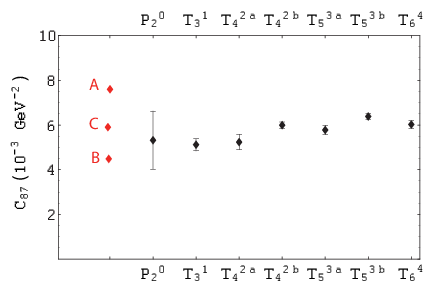
Of course, in the large- limit does not run with scale whereas in the world at it does. This is an additional source of systematic error in the result (13). However, phenomenological evidence as well as theoretical prejudice[24] suggests that a reasonable guess for this systematic error may be obtained by varying the scale in between the range (compare with in (7)). Using the running obtained in Ref. [25], this error turns out to be per cent, right in the ballpark expected for a typical effect. This systematic error should be added to our large- result in Eq. (13) in order to obtain an estimate for in the real world. In this case, all the different results in Fig. 1 can be encompassed by this error.
We would like to finish by recalling that PAs and PTAs are, in a way, two extreme versions of a rational approximant. While in the latter all poles are fixed at the physical masses, in the former the poles are left free, and they are obtained by demanding that the expansion around reproduces that of the original function to the highest possible order. Besides these two rational approximants, there are also the so-called Partial Pade Approximants[18, 22] which, from a certain point of view, lie half way between PAs and PTAs. These Partial Pades are rational functions whose polynomial in the denominator has only some of the poles preassigned but the others are left free, to be determined by the usual matching conditions at . Therefore, there is no reason why, in general, the poles of a Partial Pade should come out to be purely real66 6 Although, when complex, they always come in complex conjugate pairs. This just means that, in general, the poles of a rational approximant are not necessarily physical., unlike those of a PTA, which are of course real by construction. We have constructed seven of these Partial Pades, with a polynomial in the denominator up to fifth order in . In some of the cases the poles were actually complex, as it was also the case of the PA [18]. However, the results obtained for are almost identical to those in Fig. 1, although with errors which are somewhat larger. This feature reinforces the stability of the result shown in Fig. 1, and gives us reassurance about the reliability of our result. Finally, we would like to mention that predicting LECs may also be another straightforward application of this method.
Acknowledgements
We are grateful to M. Martinez for his instructive comments on the treatment of errors via the montecarlo method and to J.J. Sanz-Cillero for discussions. One of us (SP) is grateful to P. Gonzalez Vera, G. Lopez Lagomasino and J. Weniger for their explanations on the mathematical properties of Pade Approximants, and to C. Brezinski for a useful correspondence on the same subject. This work has been supported by CICYT-FEDER-FPA2005-02211, SGR2005-00916, the Spanish Consolider-Ingenio 2010 Program CPAN (CSD2007-00042) and by the EU Contract No. MRTN-CT-2006-035482, “FLAVIAnet”.
References
- [1] S. Weinberg, Physica A 96 (1979) 327.
- [2] J. Gasser and H. Leutwyler, Nucl. Phys. B 250 (1985) 465.
- [3] C. Aubin et al. [MILC Collaboration], Phys. Rev. D 70 (2004) 114501 [arXiv:hep-lat/0407028].
- [4] E.J. Weniger, J. Math. Phys. 45 (2004) 1209 [arXiv:math-ph/0306063], section 6.
- [5] M. Golterman and S. Peris, Phys. Rev. D 67 (2003) 096001 [arXiv:hep-ph/0207060].
- [6] G. ’t Hooft, Nucl. Phys. B 72 (1974) 461.
- [7] S. Peris, arXiv:hep-ph/0204181; E. de Rafael, Nucl. Phys. Proc. Suppl. 119 (2003) 71 [arXiv:hep-ph/0210317]. See also M. Knecht and E. de Rafael, Phys. Lett. B 424 (1998) 335 [arXiv:hep-ph/9712457].
- [8] See, e.g., R. L. Jaffe, AIP Conf. Proc. 964 (2007) 1 [Prog. Theor. Phys. Suppl. 168 (2007) 127] [arXiv:hep-ph/0701038] and references therein.
- [9] E. Witten, Nucl. Phys. B 160 (1979) 57.
- [10] H. W. Fearing and S. Scherer, Phys. Rev. D 53 (1996) 315 [arXiv:hep-ph/9408346], J. Bijnens, G. Colangelo and G. Ecker, JHEP 9902 (1999) 020 [arXiv:hep-ph/9902437].
- [11] M. Davier, L. Girlanda, A. Hocker and J. Stern, Phys. Rev. D 58 (1998) 096014 [arXiv:hep-ph/9802447].
- [12] C. Pommerenke, Pade approximants and convergence in capacity, J. Math. Anal. Appl. 41 (1973) 775. Reviewed in G.A. Baker and P. Graves-Morris, Pade Approximants, Encyclopedia of Mathematics and its Applications, Cambridge Univ. Press 1996, Section 6.5, Theorem 6.5.4, Collorary 1.
- [13] See, e.g., S. R. Sharpe, arXiv:hep-lat/9811006.
- [14] W. M. Yao et al. [Particle Data Group], J. Phys. G 33 (2006) 1.
- [15] See, e.g., C. Hanhart, J. R. Pelaez and G. Rios, arXiv:0801.2871 [hep-ph] and references therein.
- [16] J. R. Pelaez and G. Rios, arXiv:0711.4223 [hep-ph] and references therein.
- [17] W.T. Eadie et al, “Statistical Methods in Experimental Physics”, North-Holland 1971 and M. Martinez, private communication.
- [18] P. Masjuan and S. Peris, JHEP 0705, 040 (2007) [arXiv:0704.1247 [hep-ph]].
- [19] G. Colangelo and S. Durr, Eur. Phys. J. C 33 (2004) 543 [arXiv:hep-lat/0311023].
- [20] W. M. Yao et al. [Particle Data Group], J. Phys. G 33 (2006) 1.
- [21] M. Davier, L. Girlanda, A. Hocker and J. Stern, Phys. Rev. D 58 (1998) 096014 [arXiv:hep-ph/9802447].
- [22] C. Diaz-Mendoza, P. Gonzalez-Vera and R. Orive, Appl. Num. Math. 53 (2005) 39 and references therein; C. Brezinski and J. Van Iseghem, “Handbook of Numerical Analysis”, Vol. III, North Holland 1994.
- [23] S. Friot, D. Greynat and E. de Rafael, JHEP 0410 (2004) 043 [arXiv:hep-ph/0408281] and references therein.
- [24] G. Ecker, J. Gasser, H. Leutwyler, A. Pich and E. de Rafael, Phys. Lett. B 223 (1989) 425, G. Ecker, J. Gasser, A. Pich and E. de Rafael, Nucl. Phys. B 321 (1989) 311.
- [25] J. Bijnens, G. Colangelo and G. Ecker, Annals Phys. 280 (2000) 100 [arXiv:hep-ph/9907333].
- [26] G. Amoros, J. Bijnens and P. Talavera, Nucl. Phys. B 568 (2000) 319 [arXiv:hep-ph/9907264].
- [27] M. Knecht and A. Nyffeler, Eur. Phys. J. C 21 (2001) 659 [arXiv:hep-ph/0106034].
- [28] V. Mateu and J. Portoles, Eur. Phys. J. C 52 (2007) 325 [arXiv:0706.1039 [hep-ph]]. J. Portoles private communication.