Corrections to Gravity due to a Sol Manifold Extra Dimensional Space

It has been nearly ten years since the originating papers studying $TeV$ scale extra dimensions [1] appeared. After that, the phenomenological implications of extra dimensional models were extensively studied. Many of these studies are concentrated on the modifications caused on the gravitational potential due to extra dimensions [4, 7]. In general the modifications are of Yukawa type (except in Randall-Sundrum warped extra dimensional models), differing only in their strength and range. In this letter we shall investigate the modification of the gravitational potential caused by a Sol extra dimensional manifold. Sol manifolds are compact and orientable three dimensional manifolds, denoted as $M_{A}^{3}$. In the following sections we shall exploit the Sol manifolds geometric structure and the study of the Laplace equation on such manifolds. After that we compare the range of the corrections to the gravitational potential due to Sol manifolds, with the corresponding range of the corrections caused by a $T^{3}$ extra dimensional manifold.

Sol manifolds are one of Thurston’s 8 three dimensional geometries [2] (geometric structures). The geometrization conjecture is an approach to the geometry of three dimensional manifolds through general topological arguments. Actually one starts with the fact that three dimensional manifolds compose from 2-spheres or torii surfaces. According to the properties and the details of the topological gluing map of the above with $R$ or $S^{1}$, the resulting manifolds acquire homogeneous metrics (at least locally). Sol manifolds are described by one type of the 8 different homogeneous metrics.

Sol manifolds result from $SL(2,Z)$ stiffennings of torus bundles over the circle. More elaborately a theorem [6] states: given M a total bundle space of a $T^{2}$ bundle over $S^{1}$ with gluing map $\phi$ and let $A$ $\epsilon$ $GL(2,Z)$ represent the automorphism of the fundamental group of the torus $T^{2}$ induced by the gluing map $\phi$. Then the total bundle space admits a Sol geometric structure if $A$ is hyperbolic, an $E^{3}$ structure if $A$ is periodic and finally a Nil structure otherwise. $A$ is hyperbolic and gives rise to an orientable manifold if $|TrA|>2$ and we shall dwell on this choice. More formally, the Sol structure arises from the $SL(2,Z)$ stiffening of the mapping torus of a torus diffeomorphism $\phi$ [2].

Before proceeding let us make a comment on the structure of $A$. Two different hyperbolic gluings with $A_{1}\neq A_{2}$, give rise to different geometric Sol structures. For $A$ we will use the matrix representation of the form

$$A=\left(\begin{array}[]{cc}0&1\\ -1&n\\ \end{array}\right)$$

(1)

so the different classes of Sol geometric structures are classified by the integer $n$, with $|n|=|TrA|>2$. However this classification is not the only one existing [8], nevertheless this will do the classification properly in our case. Also we shall take into account only the positive eigenvalues of $A$.

Let us be more quantitative on the Sol manifold analysis. Consider the manifold $T^{2}\times\mathbb{R}$ described by the periodic coordinates $(x,y)$ for the torus, defined modulo $R$ (the radius of the compact dimensions) and $z$ $\epsilon$ $(-\infty,\infty)$ be a coordinate of $\mathbb{R}$. The combined action of the torus mapping through the hyperbolic gluing map $A$ diffeomorphism (which we denote as $\bar{\Gamma}$) is :

$$\bar{\Gamma}:\left(\begin{array}[]{c}x\\ y\\ z\\ \end{array}\right)\rightarrow\left(\begin{array}[]{c}a_{11}x+a_{12}y\\ a_{21}x+a_{22}y\\ z+2\pi R\\ \end{array}\right)$$

(2)

We give a general notation for the matrix $A$, of the form

$$A=\left(\begin{array}[]{cc}a_{11}&a_{12}\\ a_{21}&a_{22}\\ \end{array}\right)$$

(3)

but in practise we shall use the form of relation (1). As we described above, the Sol manifold, which is denoted as $M_{A}^{3}$ is the quotient of $T^{2}\times\mathbb{R}$ by the action of $\bar{\Gamma}$, that is $M_{A}^{3}\equiv T^{2}\times\mathbb{R}/\bar{\Gamma}$. It is obvious that it is a total torus bundle over $S^{1}$, with $T^{2}$ the fiber, $S^{1}$ the base space and $A$ the hyperbolic gluing map of the torus fibers. We shall describe the Sol manifolds for which the eigenvalues $\lambda$ of $A$ are positive. For the case of (1) the characteristic polynomial of the matrix $A$ reads:

$$\lambda^{2}-TrA\lambda+1=0$$

(4)

or equivalently:

$$\lambda^{2}-n\lambda+1=0$$

(5)

The solutions to equation (5) are $\lambda$ and $\lambda^{-1}$ with $\lambda+\lambda^{-1}=n=TrA$. Also the discriminant of $A$ is:

$$D=(a_{11}+a_{22})^{2}-4$$

(6)

which in our case reads:

$$D=(\lambda-\lambda^{-1})^{2}$$

(7)

In this letter we shall make use of another coordinate system $(u,v,z)$ on the Sol manifold. The $(u,v)$ are linear coordinates of the torus fibres related to an eigenbasis of the hyperbolic map $A$. These coordinates correspond to a rotated torus lattice. The action of $\bar{\Gamma}$ in the new coordinate system now reads:

$$\bar{\Gamma}:\left(\begin{array}[]{c}u\\ v\\ z\\ \end{array}\right)\rightarrow\left(\begin{array}[]{c}\lambda u\\ \lambda^{-1}v\\ z+2\pi R\\ \end{array}\right)$$

(8)

The original lattice was orthogonal while the new torus lattice is not. If $e_{u}$ and $e_{v}$ are the basis of the lattice after the action of $\bar{\Gamma}$ identification, then $(e_{u},e_{v})=|e_{u}||e_{v}|\cos\theta$ (the basis of the new lattice coincide with the eigenvectors of $A$ corresponding to the eigenvalues $\lambda$ and $\lambda^{-1}$). Also the coordinates of the fibers $T^{2}$ are not periodic anymore. So in order two pairs $(u_{1},v_{1})$ and $(u_{2},v_{2})$ define the same point on the torus lattice, the following must hold:

$$(u_{1}-u_{2},v_{1}-v_{2})=ke_{u}+me_{v}$$

(9)

with $k,m$ integers and $e_{u}$, $e_{v}$ defined previously.

The main purpose of this paper is to examine the corrections to the gravitational potential caused by an extra dimensional Sol manifold. The spacetime manifold is of the form $M^{4}\times M_{A}^{3}$. In this section we review the general technique to obtain these corrections. The presentation is based on reference [4]. The techniques that will be presented are applied to compact manifolds, since this is the case of $M_{A}^{3}$. A generalization to non-compact manifolds can be found in [5].

Consider a spacetime of the form $M^{4}\times M^{n}$, with $M^{n}$ an n-dimensional compact manifold and $M^{4}$ the four dimensional Minkowski spacetime. Suppose there exist a complete set of orthogonal harmonic functions on $M^{4}$, $\Psi_{m}$, satisfying the orthogonality condition:

$$\int_{M^{n}}\Psi_{n}(x)\Psi_{m}^{*}(x)=\delta_{n,m}$$

(12)

and the completeness relation:

$$\sum_{m}\Psi_{m}(x)\Psi_{m}^{*}(x^{\prime})=\delta^{(n)}(x-x^{\prime})$$

(13)

The functions $\Psi_{m}$ are eigenfunctions of the $n$-dimensional Laplace-Beltrami operator $\Delta_{n}$ of the manifold $M^{n}$, with eigenvalues $\mu_{m}^{2}$:

$$-\Delta_{n}\Psi_{m}=\mu_{m}^{2}\Psi_{m}$$

(14)

The gravitational potential $V_{n+4}$ satisfies the Poisson equation in $n+3$ spatial dimensions, when the Newtonian limit is taken:

$$\Delta_{n+3}V_{n+4}=(n+1)\Omega_{n+2}G_{n+4}M\delta^{(n+3)}(x)$$

(15)

with $M$, the mass of the system, $G_{n+4}$ the Newton constant in $n+4$ dimensions and

$$\Omega_{n+2}=\frac{2\pi^{\frac{n+3}{2}}}{\Gamma(\frac{n+3}{2})}$$

(16)

Equation (15) corresponds to the case of large compact radius limit and has the solution:

$$V_{n+4}=-\frac{G_{n+4}M}{r_{n}^{n+1}}$$

(17)

In the case of our interest, where the compact dimensions have small lengths, we find the harmonic expansion of $V_{n+4}$ in terms of the eigenfunctions of the product space $M^{4}\times M^{n}$, which reads:

$$V_{n+4}=\sum_{m}\Phi_{m}(r)\Psi_{m}(x)$$

(18)

with $r$ denoting the coordinates of $M^{4}$ and $x$ denoting the coordinates of $M^{n}$. Consequently, the $\Phi_{m}$ obey:

$$\Delta_{3}\Phi_{m}-\mu_{m}^{2}\Phi_{m}=(n+1)\Omega_{n+2}\Psi_{m}^{*}(0)G_{n+4}M\delta^{3}(x)$$

(19)

with solution:

$$\Phi_{m}(r)=-\frac{\Omega_{n}G_{n+4}M\Psi_{m}^{*}(0)}{2}\frac{e^{-|\mu_{m}|r}}{r}$$

(20)

Finally the gravitational potential is written as:

$$V_{n+4}=-\frac{\Omega_{n}G_{n+4}M}{2r}\sum_{m}\Psi_{m}^{*}(0)\Psi_{m}(x)e^{-|\mu_{m}|r}$$

(21)

Since all point particles in the four dimensional spacetime have no dependence on the internal compact space $M^{n}$, we can take $x=0$ in (21) to obtain the four dimensional gravitational potential:

$$V_{4}=-\frac{G_{4}M}{r}\sum_{m}\Psi_{m}^{*}(0)\Psi_{m}(0)e^{-|\mu_{m}|r}$$

(22)

which is valid for large values of $r$, compared to the lengths of the compact dimensions.

In the above general result of relation (22) we shall apply the eigenfunctions and eigenvalues of Sol manifolds. For the eigenvalues we shall take the first two smallest eigenvalues (and their corresponding eigenfunctions) since larger eigenvalues are exponentially suppressed.

In order to compute corrections to the gravitational potential we must solve equation (14) for the case of Sol manifold $M_{A}^{3}$. A much more elaborate analysis of this section can be found in [3] We shall use the $(u,v,z)$ coordinates we introduced previously. The Laplace-Beltrami operator for the manifold $M^{3}_{A}$ is:

$$\Delta=Ee^{2z\ln\lambda}\frac{\partial^{2}}{\partial u^{2}}+2F\frac{\partial^{2}}{\partial u\partial v}+Ge^{-2z\ln\lambda}\frac{\partial^{2}}{\partial v^{2}}+\frac{\partial^{2}}{\partial z^{2}}$$

(23)

which stems from the Riemannian metric (11). As usual $E=|e_{u}|^{2}$, $F=|e_{v}|^{2}$ and $G=|(e_{u},e_{v})|$, where $e_{u}$ and $e_{v}$ the basis of the $T^{2}$ lattice. Thus we must solve

$$-\Delta\psi=E\psi$$

(24)

Since the coefficients of $\Delta$ depend on $z$, the form of the solutions of (24) are of the form:

$$\Psi_{\gamma}(u,v,z)=e^{2\pi i(\gamma,{\,}w)}f(z)$$

(25)

where $\gamma$ is a vector of the dual lattice of $T^{2}$ and $w$ is a vector of the $T^{2}$ lattice. Let us note that the vector of the dual lattice $\gamma$ can be written

$$\gamma=\frac{m}{R}e_{u}^{*}+\frac{n}{R}e_{v}^{*}$$

(26)

with $e_{u}^{*}$ and $e_{u}^{*}$ the vector basis of the dual $T^{2}$ lattice. The vector of the $T^{2}$ lattice can be written:

$$w=ue_{u}+ve_{v}$$

(27)

The scalar product of $w$ and $\gamma$ is identified with the usual product between the reciprocal and the Bravais lattice. Now we shall use a proposition of reference [3], which says that a function $\Psi=e^{2\pi i(\gamma,{\,}w)}f(z)$ satisfies equation (24) if and only if $f(z)$ satisfies the modified Mathieu equation:

$$\Big(-\frac{d^{2}}{dz^{2}}+|\nu(\gamma)|\cosh 2\mu(z+\alpha(\gamma))\Big)f(z)=\Lambda f(z)$$

(28)

with $\mu=\ln\lambda$, $\nu(\gamma)=8\pi^{2}CQ_{A^{*}}(\gamma)$ and $\alpha(\gamma)=\frac{\ln\big(\sqrt{\frac{E}{G}}\frac{|(\gamma,e_{u})|}{|(\gamma,e_{v})|}\big)}{2\ln\lambda}$. Also

$$C=\frac{1}{\sqrt{D}\mathrm{Vol}(M_{A}^{3})\sin\theta}$$

(29)

The volume of the Sol manifold, ${Vol}(M_{A}^{3})$, equals the volume of the total bundle space $T^{2}\times S^{1}$. In the above $D$ is the discriminant of the matrix $A$ defined in relation (7) and $Q_{A^{*}}(\gamma)$ is the quadratic form (see [3]) corresponding to the matrix $A^{*}$ acting to the dual lattice of $T^{2}$, with $Q_{A^{*}}(\gamma)=(\gamma,e_{u})(\gamma,e_{v})(\lambda-\lambda^{-1})$. The eigenvalues $E$ and $\Lambda$ are related as follows:

$$E=\Lambda+\nu(\gamma)\cos\theta$$

(30)

It is proved in reference [3] that the functions $\Psi_{\gamma}=e^{2\pi i(\gamma,{\,}w)}f_{\gamma}(z)$ form a complete orthogonal basis on the Sol manifold. Also it is found that the spectrum of the Laplace-Beltrami operator consists of two parts:

• •

  The trivial part, with eigenvalues $E_{k}=\frac{4\pi^{2}k^{2}}{R^{2}}$, corresponding to $\gamma=0$ in the dual lattice and to eigenfunctions $e^{i2\pi kz/R}$, $k=0,1,...$.

• •

  The non-trivial part with eigenvalues $E_{k,[\gamma]}=\Lambda_{k}(\nu[\gamma])+\nu([\gamma])\cos\theta$ and eigenfunctions the solutions of (28).

In order to compute corrections to the gravitational potential due to Sol structure of extra dimensions, we must compute the first eigenvalues and eigenfunctions. We shall use the most interesting case which is when $Vol(M_{A}^{3})\sin\theta$ is large (or equivalently $\nu\rightarrow 0$). Bear in mind that this term contains the compactification radius of the extra dimensions (we must state that the radii of all extra dimensions shall be considered equal) and the deformation of the lattice in terms of $\theta$. Following [3] when $Vol(M_{A}^{3})\sin\theta$ becomes large, $\nu(\gamma)$ becomes small. In that limit the eigenvalues of the Laplace-Beltrami operator, stemming from the non-trivial part, are $E_{k}=\Lambda_{k}$, with $\Lambda_{k}$ the eigenvalues of the modified Mathieu operator,

$$M=-\frac{d^{2}}{dz^{2}}+|\nu(\gamma)|\cosh 2\mu z$$

(31)

We order the first eigenvalues as $E_{0}=0\leq E_{1}\leq E_{2}\leq...$. We shall use the first two, since the corrections to the gravitational potential fall exponentially at the eigenvalues grow larger. Thus the first two are $E_{0}=0$ and $E_{1}$, which asymptotically reads:

$$E_{1}\sim\frac{(\ln\lambda)^{2}\pi^{2}}{(\ln C)^{2}}$$

(32)

with $C$ as before:

$$C=\frac{1}{\sqrt{D}\mathrm{Vol}(M_{A}^{3})\sin\theta}$$

(33)

The eigenfunctions corresponding to the Mathieu operator (31) are in general,

$$f_{m}(z)=\sum_{k=0}^{\infty}A_{2k}^{2m}\cosh[2kz]$$

(34)

with ${}^{\prime}m^{\prime}$ counting the eigenvalues, $m=0$ corresponds to $E_{0}$ e.t.c.

Now we are ready to compute the modifications to the gravitational potential coming from the first two eigenvalues of the Laplace operator on Sol manifolds. Thus we substitute $E_{0}$ and $E_{1}$ in relation (22) with $|\mu_{0}|=\sqrt{E_{0}}$ and $|\mu_{1}|=\sqrt{E_{1}}$. Also we substitute the eigenfunctions for the Sol manifold, thus:

$$\Psi_{m}(0)=\sum_{k=0}^{\infty}A_{2k}^{2m}$$

(35)

The asymptotic behavior of the coefficients $A_{2k}^{2m}$ for $\nu\rightarrow 0$ (which is the most interesting case and we shall dwell on it) is really simple [9]. It turns out that the terms of the form $A_{m}^{(m)}$ tend to $1$, while terms of the form $A_{m}^{(k)}$, with $m\neq k$ tend to zero. Thus the gravitational potential of relation (22) becomes:

$$V_{4}=-\frac{G_{4}M}{r}\sum_{m}\sum_{k=0}^{\infty}A_{2k}^{2m}A_{2k}^{2m}e^{-|\mu_{m}|r}$$

(36)

So for the first two eigenvalues we have

$$V_{4}=-\frac{G_{4}M}{r}\Big(A_{0}^{0}A_{0}^{0}e^{-|E_{0}|r}+A_{2}^{2}A_{2}^{2}e^{-|E_{1}|r}\Big)$$

(37)

or (using the asymptotic behavior for the coefficients $A_{m}^{(m)}$):

$$V_{4}=-\frac{G_{4}M}{r}\Big(e^{-\sqrt{E_{0}}r}+e^{-\sqrt{E_{1}}r}\Big)$$

(38)

Since $E_{0}=0$ and using relations (32) and (33) we obtain finally:

$$V_{4}\sim-\frac{G_{4}M}{r}\Big(1+e^{-\big|\frac{(\ln\lambda)\pi}{(\ln C)}\big|r}\Big)$$

(39)

In the relation above it is clear that the Sol manifold correction to the Newton’s law gravitational potential depends on the compactification radii of the extra dimensions $R$, the angle $\theta$ of the vectors $e_{u}$ and $e_{v}$ and on the eigenvalues of the hyperbolic gluing map $A$. In the next section we shall investigate the parameter space of the corrections found (which is very rich) and we shall compare it with the $T^{3}$ manifold corrections, to see how much different these are.

The parameter space of the Sol correction to the gravitational potential is very rich. Let us examine first the dependence of the Sol correction range $e^{-\mu_{m}r}$ on the parameters $\theta$ and $n$. In Figure (6) we plot the dependence for the compactification radius value $R=0.05{\,}mm$ (smaller than the current experimental bound $r=0.2mm$) and for $r=0.1{\,}mm$, while in Figure (7) and (8) the values of $R$ are $0.1{\,}mm$ and $0.2{\,}mm$ respectively. We tried to check the plots near the experimental bound for extra dimensions. It seems that the Sol structure gives very large corrections to gravity if the compactification radius is very small (of order $R\sim 10^{-6}{\,}$ and smaller). We shall study the interesting cases which have compactification radius around $R\sim 0.2{\,}mm$. Also we shall check out the behaviour of the range of the corrections around $R\sim 10^{-8}m$ which is the expected scale that three extra dimensional spaces should have. Looking in Figures (6), (7), and (8), we can see that the last two have similar dependence. It seems that for large values of $n$ ($>200$) and for $\theta>0.3$, the corrections are very small. In the other two graphs when $n>300$ and for small values of $\theta$, the corrections are small. In the following we shall investigate some interesting cases stemming from the above three. To have a clear picture we shall compare the range of Sol manifolds with the range of the $T^{3}$ torus corrections.

In Figure (9) we plot the range of the $T^{3}$ corrections as a function of $r$ with $R=0.05mm$ and $\theta=\pi/3$ and in Figure (10) the corresponding dependence for the Sol manifold case. As expected from Figure (6), the term $e^{-\mu_{m}r}$ is very big compared to $e^{-r/R}$, for small $n$ ($\sim 5$). As $n$ grows the term becomes smaller and smaller. Figure (10) corresponds to $n=250$. As $n$ grows, the range of Sol-corrections becomes comparable and after a value of $n$, smaller compared to the $T^{3}$ corrections. The small $\theta$ case is similar. Concluding the above investigation we could say that the Sol range values are big for the above case in which the corresponding torus range values were small.

The case with $R=0.2$ mm is very interesting. As we can see in Figure (3) the range of Sol corrections can vary significantly depending on the value that $n$ takes. Compared to the corresponding 3-Torus range, Sol corrections can be much larger (for small $n$) and comparable (for $n>450$) but never smaller even for very large $n$.

Another result is that general Sol corrections can exist for compactification radii and at distances for which the corresponding $T^{3}$ torus range values are very large (and consequently not experimentally preferable).

In extra dimensional models, gravity behaves exactly as in four dimensional models when long distances are considered. When however we are close at the scale of the extra dimensions, the potential changes and we expect macroscopical changes in the strength and range of the gravitational force. This is expressed by the relation

$$M_{Pl}^{2}=M_{*}^{n+2}(2\pi R)^{n}$$

(40)

Depending on the topology and geometry of the extra dimensions, the corrections may vary.

There exist several bounds constraining the size and number of extra dimensions. For gravitational corrections the strongest constraint comes from the Eöt-Wash experiment. The results show consistency with Newtonian gravity down to 200 microns [10].

In the ADD model the scale $M_{*}$ is taken to be 1 TeV. For this value we obtain the following sizes for extra dimensions with the same radius $R$:

number of extra dimensions	R (m)
n=1	$\sim 10^{12}$
n=2	$\sim 10^{-3}$
n=3	$\sim 10^{-8}$

The case of one extra dimension with quantum gravity scale $\sim$1 TeV is ruled out by solar system experiments. Also two extra dimensions are ruled out since for $M_{*}$=1 TeV the experiments have tested Newton’s force down to 200 microns.

Bounds on extra dimensions are posed when gravitons are taken into account. Gravitons would be copiously produced in colliders unless $M_{*}$=1 TeV for $n=3$. There exist stronger bounds when light gravitons are taken into account. These are emitted from supernovae and the astrophysical bounds for three extra dimensions on $M_{*}$=1 TeV are of the order TeV [11].

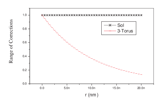
In the case of Sol manifolds the same arguments hold and also, due to the toroidal fibration, equation (40) is valid (the only difference might be in some graviton cross-sections because the distribution of eigenvalues of the Laplacian on Sol manifolds is such that leads to non-constant mass splitting. In fact the eigenvalue distribution is not Poisson, as for most toric topologies happens. This will be studied elsewhere). Sol space is three dimensional. Taking into account that the experimental and theoretical bound is $R=10$ nm, we compare the range of the three torus corrections and the range of Sol manifolds corrections. In Figure (1) we plot the range of the two manifolds.

As we can see, the range of the Sol corrections is significantly larger from the three torus corrections. Also the range of the $T^{3}$ corrections drop much faster compared to the Sol case. This is very interesting phenomenologically. In the Sol case, the values of the corrections are too close one to each other and in Figure (1) appears as a straight line (but it is not). In addition we found that the values of $n$ (the parameter appearing in the $SL(2,Z)$ matrix) and of $\theta$, do not seem to modify the results significantly, for $R\sim 10^{-8}{\,}$ m. The last is to be contrasted with the case $R\sim 0.2$ mm as can be seen in Figure (3).

As we can see the $n$ value modifies significantly the range of Sol corrections when $R\sim 0.2$ mm. For large $n{\,}(\sim 450)$ the Sol corrections are comparable to the 3-torus corrections while for small $n$ the range of Sol corrections grow larger and larger.

Let us return to the case $R\sim 10^{-8}$ m and see how the modifications behave down to the $200{\,}\mu$m ($0.2$ mm). We found that in the 3-torus case, the range of the corrections becomes extremely small for distances $r\sim 10^{-6}$m and smaller, while the Sol corrections for $r\sim 10^{-6}$m still remain significantly larger compared to the torus case, as can be seen in Figures (2) and (4). In the case of Sol corrections we can see that around $10^{-4}$ m and lower, the corrections become small as can be seen in Figure (5) (although the range still remains significantly larger compared to the 3-Torus case).

A more complete investigation for small $R$ would require a numerical calculation of the eigenvalues of the Sol manifold Laplace-Beltrami operator. There exists an algorithm that calculates numerically the eigenvalues of three dimensional manifolds and can be found in [13] and references therein.

In this letter we studied the corrections to the gravitational potential caused by an Sol manifold extra dimensional compact space. Specifically we used the first two eigenvalues of the Laplace-Beltrami operator on the Sol manifold which showed us that the Yukawa type modifications are affected by the parameters $n$, $\theta$ and $R$, where $R$ the compactification radius and $\theta$ the angle between the basis vectors of the $T^{2}$ lattice. The parameter $n$ is connected with the matrix $A$ $\epsilon$ $SL(2,Z)$, which is hyperbolic and defines the gluing of the torus fibers. After investigating the parameter space we found interesting results, mainly concluding that the range of Sol structure corrections can be similar to the $T^{3}$ torus results and (more interestingly) can be very different to the $T^{3}$ results depending to the values of the parameters. This is valuable phenomenologically as can be seen in the previous sections.

Also let us discuss the fact that for Sol manifolds, when $R$ is small, the range of the corrections is large compared with the 3-torus case. This must have to do with the intrinsic hyperbolicity of Sol manifolds. This intrinsic hyperbolicity has effect on the eigenvalues and their distribution. Due to this if we wish to take the limit $R\rightarrow\infty$ we must be very careful. In the limit $R\rightarrow\infty$ the eigenvalues grow smaller and smaller much more faster than in the 3-torus case. Thus roughly we could say that Newton’s law is recovered. However for large $R$ we must take into account the eigenvalues we disregarded since we still work in a compact space but $R$ is not small anymore. Some eigenvalues of Sol (not trivial to be found) can be found in Ref.[3].

As a final remark let us note that the values of the range of the Sol corrections remain very large compared to the 3-Torus ones (almost flat even at $R\sim 0.2$mm !). This happens even near the experimental limits $0.2$ mm. At first this may appear very strange but the study involved only the range of the corrections, so the large range values might be interesting feature since the range is divided by the distance $r$. Thus in some cases the corrections might be measurable. However extra care must be taken when $R$ is small, as we mentioned previously.

Finally we left unanswered two issues, the graviton production and how do we distinguish Sol manifolds corrections from other corrections (the last due to the rich parameter space of Sol manifolds). We hope we address these in the future.

V.O would like to thank Alex Kehagias for reading the manuscript and for valuable comments and prospective extensions of the above he gave. Also would like to thank both the referees for invaluable comments and suggestions that improved significantly the quality of the paper.

References

- [1] I. Antoniadis, N. Arkani-Hamed, S. Dimopoulos, G. R. Dvali, Phys. Lett. B436, 257 (1998)
- [2] W. P. Thurston, Three-Dimensional geometry and Topology Vol.1, Princeton University Press (1997)
- [3] A. V. Bolsinov, H. R. Dullin, A. P. Veselov, Commun. Math. Phys. 264, 583 (2006)
- [4] A. Kehagias, K. Sfetsos, Phys. Lett. B472, 39 (2000)
- [5] A. Kehagias, J. G. Russo, JHEP, 0007, 027 (2000)
- [6] M. Tanimoto, Class. Quant. Grav. 18:479, (2001)
- [7] E. G. Floratos, G. K. Leontaris, Phys. Lett. B465, 95 (1999)
- [8] H. Kodama, Prog. Theor. Phys. 99, 173 (1998)
- [9] N. W. MacLachlan, Theory and Applications of Mathieu Functions, Dover (1964)
- [10] C. D. Hoyle, D. J. Kapner, B. R. Heckel, E. G. Adelberger, J. H. Gundlach, U. Schmidt, H. E. Swanson, Phys. Rev. D70, 042004 (2004)
- [11] S. Cullen, C. Grojean, L. Pilo, J. Terning, Phys. Rev. Lett. 83, 268 (1999)
- [12] Graham. D. Kribs, Tasi 2004 Lectures on the Phenomenology of Extra Dimensions, hep-ph/0605325
- [13] N. J. Cornish, D. N. Spergel, math.DG/9906017