Non-commutative geometry inspired higher-dimensional charged, black holes Thanks: As this paper was nearing completion our friend Gallieno Denardo has suddenly passed away. As his former students, we dedicate this paper to his memory and strongly believe that without his early influence it probably would have never been written.
Abstract
We obtain a new, exact, solution of the Einstein’s equation in higher dimensions. The source is given by a static spherically symmetric, Gaussian distribution of mass and charge. The resulting metric describes a regular, i.e. curvature singularity free, charged black hole in higher dimensions. The metric smoothly interpolates between Reissner-Nordström geometry at large distance, and deSitter spacetime at short distance. Thermodynamical properties of the black hole are investigated and the form of the Area Law is determined. We study pair creation and show that the upper bound on the discharge time increases with the number of extra dimensions.
1 Introduction
By now, it can be safely claimed that string theory induced
non-commutative geometry [1]provides an effective framework to study short distance
spacetime dynamics. The original
idea, revived by the today stringy formulation, dates back to
Snyder seminal paper [2]. In this model
there exist a universal minimal length scale. At distances near
the classical concept of smooth
spacetime manifold breaks down. It is generally assumed that
is closed to the Planck length, and as such it would be unaccessible both
to present and future experimental observations.
A promising alternative to the Planck scenario has been proposed, recently,
based on the presence of “large
extra-dimensions”. It allows to lower unification scale, i.e. string
tension, down to
energy so that stringy effects could be soon observed
at LHC [3]Thus,if non commutative geometry is induced by string theory, the
corresponding length scale should be lowered as well.
These ideas offer exciting , near future, possibility of experimentally
probing both non-commutativity and quantum gravity effects.
The most convincing confirmation of Quantum Gravity would
be the production of a mini black hole (BH) in hadronic collisions
[4],[5],[6][7]. An unambiguous signature of such an event
is based on a detailed analysis of both decay products and of the
eventual BH remnant. So far the standard scenario
of BH evaporation offered a detailed and definite predictions
for the spectrum of emitted particles, while it is inconclusive
about the final phase of BH evaporation. This ambiguity can be traced back
to the semi-classical description of Hawking process
in the sense that matter emitted by BH is
represented by quantum field theory in curved spacetime, while BH
itself is still a classical background geometry. On the other hand,
the final stage of BH decay requires quantum
gravity corrections which the semi-classical model is unable to
provide.
In view of the “quantum” character of non-commutative
geometry, one expects that in this model the late stage of the evaporation
is determined by spacetime fluctuations when the radius of the BH horizon
becomes comparable with . Usual attempts to obtain BH solutions
of “non-commutative” Einstein’s equations are based upon perturbative
expansion in the parameter. So far, all these attempts lead
to unconvincing results: it is unacceptable that curvature singularities
can survive coordinate fluctuations in spite of the
existence of a minimal length
[8].It is likely that these problems are due to the method of
approximating the original, intrinsically non-local theory, with a local
truncated expansion of the action functional in terms of derivative
interactions.
Against this background, we proposed an approach based on
“quasi-classical coordinates”, keeping track
of the intrinsic non-locality in the form a minimal length in the
spacetime fabric.
As a result, matter/energy densities are described by
minimal width Gaussian distributions, in complete agreement with the basic
principles of quantum mechanics. Solutions of Einstein’s equations with
such smeared sources give new kind of regular BHs
in four [10]and higher dimensions [11].
These models lead to new predictions for the final stage of
Hawking evaporation. End result is a massive remnant in the form of
a neutral, cold, near-extremal BH. The mass of this residual and
stable object is determined by the parameter.
Its eventual observation
would be an unambiguous experimental signature pointing out that:
i) a BH has been produced in the hadronic collision;
ii) there exists a minimal length inherent to short distance
spacetime structure [14][15].
Motivated by this exciting perspective, we present
in this paper a detailed study of the higher dimensional,
charged, regular, mini BH.
2 Higher dimensional solution
Before we engage in a detailed calculation we would like to point out
the basic idea of our implementation of non-commutative effects.
It would be desirable to formulate non-commutative theories,
including General Relativity, directly in terms of non-commuting
coordinates. This approach would correspond to a new, deeper, level
of “quantization” acting on the spacetime manifold itself rather
than on fields, including the metric, which are structures assigned
over the manifold itself. Unfortunately a framework of this type is not
presently available.
In a non-commutative geometry, familiar concepts loose their very meaning.
As an example, it is worth to remark a problem
that seems to be ignored in the current literature
[8]while it should be especially evident when facing
non-commutative extensions of General Relativity. Coordinate
non-commutativity implies the existence of a finite
minimal length , below which the very concept of
“distance” becomes physically meaningless.
Such a basic remark, immediately, raises the problem to
define the line element, namely the infinitesimal distance
between two nearby points in Einstein gravity. One possible way around
is to adopt Weyl-Wigner-Moyal product [16],
paying the cost of possible violation of
unitarity [17]
and Lorentz invariance in ordinary quantum field theory,
or anisotropy of the Newton gravitational potential
11
1
The alternative approach in terms of coordinate coherent
states leads to a spherical symmetry preserving, short distance modification
only of the Newton potential [19][18].
Furthermore, star-product formulation of non-commutative quantum field
theory can be handled only through perturbative
expansion in the parameter. At any finite order in
the approximated theory keeps no memory of its original non-locality
and looks like an ordinary quantum field theory affected
by higher order derivative self-interactions. The original UV cut-off
is turned into a dimensional coupling constant leading
to a non-normalizable UV behavior even worse than in ordinary quantum
field theory.
For all these reasons, we have developed an effective approach
where non-commutativity is implemented only through a Gaussian de-localization
of matter sources. In this way there is no problem in defining line
element and Einstein’s equations are kept unchanged. Our strategy can be
summarized as follows:
i) in non-commutative geometry there cannot be point-like object, because
any physical distance cannot be smaller than a minimal position uncertainty
of the order of ;
ii) this effect is implemented in spacetime through matter
de-localization, which by explicit calculations
[20]turns out to be of Gaussian form;
iii) Spacetime geometry is determined through Einstein’s equations with
de-localized matter sources;
iv) de-localization of matter backfires at spacetime geometry giving
regular, i.e. curvature singularity free, metrics. This is exactly
what is expected from the existence of a minimal length.
The presence of a universal short distance cut-off leads to the following
effects: in quantum field theory it cures UV divergences
[21]; in General Relativity
it cures curvature singularities [10, 22].
In view of the above explanations, we are going to solve the resulting
Einstein’s equations,
in higher dimensions, with a maximally localized source of energy and
electric charge. The corresponding distributions have a minimal
spread Gaussian profile
| (1) | |||||
| (2) |
Matter and charge density in Eq.(1), (2) model a
physical source which is as close as it is possible to a
“point-like” object. is the “bare mass” and
is the total electric charge. We remark that
is only part of the total mass-energy of the system.
The Coulomb energy stored in the electric field is a second contribution
to the total mass-energy sourcing the gravitational field.
We are looking for static, spherically symmetric gravitational and
electric fields solving the coupled field equations
| (3) | |||
| (4) | |||
| (5) |
where the Greek indices , , etc. run over ;
is the reduced fundamental scale for
i.e. , while
for , i.e. .
is the higher dimensional extension of the
energy-momentum tensor described in [10];
is charge current which has -component non-vanishing.
The Coulomb-like field satisfying the equation (5) results to be
| (6) |
where, is the Euler lower Gamma function defined by the following integral representation:
| (7) |
It turns out that the electric field is linearly vanishing
for independently of the number of space dimensions.
On the other hand, the large distance behavior is sensitive to
extra dimensions and falls-off as .
In order to proceed, we insert solution (6)
in the electromagnetic energy momentum tensor and
solve Einstein’s equations (3 ). We find
Reissner-Nordström like form of the metric :
| (8) | |||
| (9) |
The main feature of (8) is the absence of curvature singularities. To prove this statement in a simple and painless way, we consider the short-distance behavior of the metric. Inserting the small argument expansion of (7) in (8), the geometry near the origin is given by
| (10) | |||
| (11) |
One recognizes in (10) deSitter spacetime, which is known to
be singularity-free. Equation (11) shows as the bare mass
and the noncommutative parameter mix together to produce
an effective cosmological constant . It is not
surprising that different mass particles experience different cosmological
constants. The deSitter vacuum represents the geometrical counterpart
of the underlying noncommutative coordinate fluctuations which are taking place
over a distance scale defined by . Different values of
imply different Compton wavelength and “resolution power”.
Heavy particles can probe shorter distance better than light objects,
and result to be more sensible to spacetime quantum fluctuations.
In our solution the curvature singularity smears into a regular, fluctuating,
vacuum core which is quasi-classically described by a deSitter geometry.
Short-distance spacetime fuzziness, once it is implemented through our quasi-classical geometrical method,
cures curvature singularity as it was anticipated in the Introduction.
In order to proceed in our investigation, it is convenient to define the radial mass-energy ,
accounting for both Coulomb and matter energy contributions
| (12) |
The total mass-energy, , measured by an asymptotically distant observer is given by
| (13) |
Solution 8) is now expressed in terms of as
| (14) | |||||
| (15) |
As one might expect, at distance , Equation(8) gives ordinary m-dimensional Reissner-Nordström metric
| (16) |
At this point, it is important to address the problem of the existence of event horizons. Their position is determined by the roots of the equation . In our case horizon equation cannot be solved analytically, but a plot of as a function of , for fixed values of , , determines the positions of horizon(s).

For any there can be two horizons
when , one degenerate horizon
for , or no horizon if . is the mass of an
extremal BH and represents its final
state at the end of Hawking evaporation process. The details will be given in
next Section. Furthermore, it
results that increasing , more and more mass is needed to create
a black hole of a given radius.
The global properties of the analytically
extended solution across the horizon (coordinate singularities)
can be obtained by gluing together outer Reissner-Nordström and
inner deSitter patches.
On general ground horizons are solutions of the equation
| (17) | |||
| (18) |
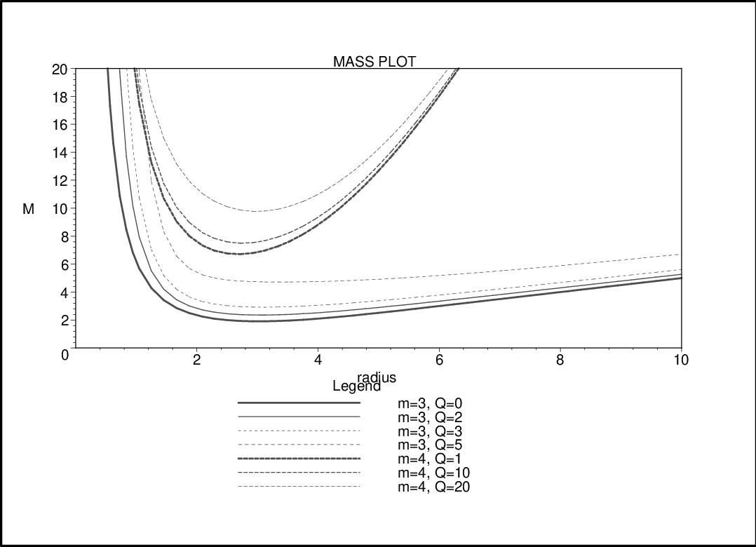
Eq.(18) offers an alternative way of studying existence of
horizons.
The use of the equation relating
the total mass energy of the system to the radius of the event
horizon follows the approach proposed in
[23]with the advantage of allowing
an in-depth investigation of geometry and dynamics of the system.
We see that the sole effect of extra-dimensions
is to lift upward the dimensional curve thus increasing
the value of the mass for a given radius of the horizon, including
the degenerate case. Thus, we conclude that the evolution of the
BH towards its extremal configuration is qualitatively the same as
described in [10]. The increase of the mass
and its eventual experimental verification could indicate
the number of extra-dimensions.
3 Black hole thermodynamics
In this section we are going to investigate some thermodynamic properties of the regular BH described by the line element (8). The starting point is the explicit form of the Hawking temperature :
| (19) |
where, we replaced with by using the horizon equation (18).

From the plot of the temperature one sees that in any dimension there is
an initial “ Schwarzschild-phase ” for .
Approaching maximum temperature, a departure from the Schwarzschild behavior
shows up. The maximum temperature occurs in the range . Immediately after the temperature drops down
and the BH enters a nearly-extremal phase, asymptotically approaching
a zero-temperature, degenerate configuration.
This is the same behavior already encountered in the neutral
case [10].
The effect of extra-dimensions is to shift upwards
the temperature while shrinking the radius of the extremal BH.
The effect of charge is just to lower the temperature as can be
seen from the two curves with and .
Therefore, upper bounds for the maximal temperature can be obtained from
the plot of in the neutral case.
One can see from (19) that the peak temperature increases with ,
but even in the case it is
about which is much lower than
.
For i.e. no extra-dimensions, the fundamental
scale . Notwithstanding, back-reaction is still negligible as
the maximal temperature is much lower than .
| m | 3 | 5 | 6 | 9 | 10 | |||||
|---|---|---|---|---|---|---|---|---|---|---|
| (TeV) | 2.3 | |||||||||
| ( fm) |
The energy of the electrostatic field increases the total mass-energy. Thus,
the minimal value for as a
function of can be obtained studying the neutral case . This is given
in Table (1), where we
also listed the corresponding radius of the event horizon. The BH production
cross section is simply the area of
the event horizon, which leads to an estimate of the order of , for
every . This is “good news”. On
the other hand, the “bad news” is that for the remnant is too heavy
to be produced at LHC
[11]. Maybe, these kind of objects could be detected in
Ultra-High-Energy cosmic rays
[12, 13].
In this section we are also going to investigate
eventual effect of the minimal length on the expression of the BH entropy
[24]in terms of the area of the event horizon.
It can be useful to recall
that the celebrated area/entropy law was originally derived by Bekenstein
in the framework of information theory. The correct proportionality constant
between entropy and area of the event horizon was later obtained by
Hawking through a thermodynamic approach. It can be worth to remark that
this relation holds for classical 22
2
Quantum effects introduce
logarithmic corrections., black, point-like, singular, objects, and there is
no a priori evidence that it would keep the same form in our case. We
must derive it “from scratch”, so to say. Under this respect,
the thermodynamic approach is easier to carry out. We start from
the fundamental law of black hole thermodynamics
where, is the electrostatic potential
on the event horizon.
As physical quantities are evaluated on the event horizon,
can be expressed in terms of and
can be written as
| (20) |
From the two different forms of one finds the following expression for the BH entropy
| (21) |
We start from (18) and calculate
is confronted with the expression (19) for the BH temperature leading to the relation
| (22) |
The final expression for the BH entropy variation is
| (23) |
In order to obtain the BH entropy we integrate (23) from the extremal horizon up to a generic external horizon . The result is
| (24) |
Taking into account that the area of the event horizon is we rewrite (24) as
| (25) | |||
| (26) |
The first term in equation (25) generalizes the celebrated four
dimensional relation to higher dimensions. It is worth noticing
that the Newton constant is replaced by the effective gravitational coupling.
A similar conclusion has been recently attained, in a different framework, in
[25].
Finally, let us analyze in more details correction term
in (25).
It can be seen that always,
so we can approximate and write ( in Planck units )
| (27) |
We conclude that the area law is maintained up to exponentially small
corrections.
We have shown that the temperature of a
Reissner-Nordström type BH never diverges.
Thus, the end-point of the Hawking evaporation is a nearly extremal BH in
thermal equilibrium with the
environment. However, in the four dimensional picture
this is not a satisfactory candidate to the role of remnant because
charged BHs results to be quantum mechanically
unstable under pair production. A mini BH decays into a neutral
Schwarzschild type object much before reaching a significant temperature.
Once in the Schwarzschild phase the temperature will increase without
limit leading to an unpredictable final stage. This is not a problem
in our case thanks to the presence of the parameter even in
neutral phase.
4 Pair creation
In this section we are going to study the discharge process with
a special attention to the way the presence of extra dimension
affects the mean life of the charged object.
The creation of pairs near the event horizon is
described by the Schwinger formula [26].
This formula implies
that in order for creation process to take place, the electric field
has to exceed the critical intensity .
Over-criticality condition leads to
| (28) |
The concept of Dyadosphere has been introduced in [27, 28] as the spherical region, of radius , where (28) is valid. Recently, there has a criticism about the possibility of Dyadosphere development for astrophysical objects [29]. Without going into this debate, we would like to notice that in the case of micro BH the condition for the existence of the Dyadosphere is always met in any dimension. In our case, the radius is determined by
| (29) |
Equation (29) can be solved numerically. However, in what follows we do not need the explicit value of . In order to proceed, we introduce a surface charge density as:
| (30) |
The idea is to divide the Dyadosphere into “thin” spherical
shells of thickness equal to the electron Compton wavelength
. Within each shell the electric field can be considered
constant and described by
.
Such a description in terms of constant field is necessary in order to
apply the Schwinger formula.
The critical surface density is obtained when :
It can be inferred from Fig.(1) and the definition
(29) that . Thus,
we see that the dependence of the critical density from is
confined only within the electric charge.
For -pairs are created and
the rate of their production is given by
| (31) |
The total number of pairs produced, in one second, inside a spherical shell of thickness is
| (32) |
The discharging process is taking place until the critical density is reached. Then, it becomes exponentially suppressed. The decay time can be obtained by noticing that
| (33) |
Thus, we estimate the discharge time to be
| (34) |
where, we introduced the variable . In order to restore the dependence from the minimal length let us recall that the electric charge is a dimensional quantity. Thus, we write where, is the fine structure constant in four dimensions, and is a characteristic length scale of the higher dimensional theory. In our approach there is only one length scale and it is natural to identify . Then, the discharge mean time turns out to be (in c.g.s. units )
| (35) |
where we estimate , which is compatible with expected length scale in quantum gravity. Eq.(35) gives the discharge time assuming that the process takes place in the dimensional bulk spacetime. It is interesting to compare it with corresponding expression for which describes pair creation on the “three-brane” world. Thus we find
| (36) |
An upper bound on can be obtained for , i.e. , and [28]:
| (37) |
As there are no evidence of the presence of a minimal length at the
atomic length scale, . Eq.(37) shows that
both and
contribute to the increase of the mean life by several orders of magnitude,
already for slightly greater than three.
We conclude that: if the decay takes place in the bulk the discharge
time increases significantly as a function of . If, on the contrary,
brane universe scenario, where standard model elementary particles are
confined on the brane, is realized in nature should be
of the order of .
Two comments are in order. From (37) we see that
Schwinger mechanism is relevant only in the case . For
higher dimension charge neutralization will take place through
Hawking emission, as soon as the BH temperature is higher than
, and
capture of surrounding charged particles produced in the
hadronic collision. Secondly, our considerations assume electrons
to be free to move in the whole higher dimensional space.
Brane models constrain ordinary matter particle to be glued
to the brane itself, while only gravity can probe transverse
higher dimensions. Even if a D-brane is not explicitly present in our
geometry, line element (8) can approximate a D-brane geometry
provided the radius of the event horizon is small with respect to
the size of the extra dimensions. To take into account models where
gauge fields are confined to the brane, Schwinger mechanism must
be restricted to take place only inside the brane and the relevant
discharge time is given by .
References
- [1]
E. Witten,
Nucl. Phys. B 460, 335 (1996)
[arXiv:hep-th/9510135]
N. Seiberg and E. Witten, JHEP 9909, 032 (1999) [arXiv:hep-th/9908142] ������� - [2] H. S. Snyder, Phys. Rev. 71, 38 (1947)
- [3]
N. Arkani-Hamed, S. Dimopoulos and G. R. Dvali,
Phys. Lett. B 429, 263 (1998)
[arXiv:hep-ph/9803315]
I. Antoniadis, N. Arkani-Hamed, S. Dimopoulos and G. R. Dvali, Phys. Lett. B 436, 257 (1998) [arXiv:hep-ph/9804398] - [4]
S. B. Giddings,
in Proc. of the APS/DPF/DPB Summer Study on the Future of Particle Physics
(Snowmass 2001) ed. N. Graf,
In the Proceedings of APS / DPF / DPB Summer Study on the Future of
Particle Physics (Snowmass 2001), Snowmass, Colorado, 30 Jun - 21 Jul
2001, pp P328
[arXiv:hep-ph/0110127]
M. Bleicher, S. Hofmann, S. Hossenfelder and H. Stoecker, Phys. Lett. B 548, 73 (2002) [arXiv:hep-ph/0112186]
M. Stenmark, Chin. J. Phys. 40 (2002) 512
S. D. H. Hsu, Phys. Lett. B 555, 92 (2003) [arXiv:hep-ph/0203154]
M. Cavaglia, S. Das and R. Maartens, Class. Quant. Grav. 20, L205 (2003) [arXiv:hep-ph/0305223]
A. Chamblin, F. Cooper and G. C. Nayak, Phys. Rev. D 70, 075018 (2004) [arXiv:hep-ph/0405054]
M. Cavaglia and S. Das, Class. Quant. Grav. 21, 4511 (2004) [arXiv:hep-th/0404050]
S. Shankaranarayanan and N. Dadhich, Int. J. Mod. Phys. D 13, 1095 (2004)
T. G. Rizzo, Class. Quant. Grav. 23, 4263 (2006) [arXiv:hep-ph/0601029].
T. G. Rizzo, “TeV-scale black holes in warped higher-curvature gravity” arXiv:hep-ph/0510420. - [5] A. Casanova and E. Spallucci, Class. Quant. Grav. 23, R45 (2006) [arXiv:hep-ph/0512063].
- [6]
G. L. Alberghi, R. Casadio, D. Galli, D. Gregori, A. Tronconi and V. Vagnoni,
arXiv:hep-ph/0601243
R. Casadio and B. Harms, Int. J. Mod. Phys. A 17, 4635 (2002) [arXiv:hep-th/0110255]. - [7] H. Stoecker, J. Phys. G 32, S429 (2006).
- [8]
F. Nasseri,
Gen. Rel. Grav. 37, 2223 (2005)
[arXiv:hep-th/0508051]
F. Nasseri, Int. J. Mod. Phys. D 15, 1113 (2006) [arXiv:hep-th/0508122]
S. Kar and S. Majumdar, Int. J. Mod. Phys. A 21, 6087 (2006) [arXiv:hep-th/0510043]
M. Chaichian, M. R. Setare, A. Tureanu and G. Zet, “On Black Holes and Cosmological Constant in Noncommutative Gauge Theory of Gravity,” arXiv:0711.4546 [hep-th]
M. Chaichian, A. Tureanu and G. Zet, “Corrections to Schwarzschild Solution in Noncommutative Gauge Theory of Gravity,” arXiv:0710.2075 [hep-th] - [9]
A. Kobakhidze,
“Noncommutative corrections to classical black holes,”
arXiv:0712.0642 [gr-qc]
P. Mukherjee and A. Saha, arXiv:0710.5847 [hep-th] - [10]
P. Nicolini, A. Smailagic and E. Spallucci,
Phys. Lett. B 632, 547 (2006)
[arXiv:gr-qc/0510112]
S. Ansoldi, P. Nicolini, A. Smailagic and E. Spallucci, Phys. Lett. B 645, 261 (2007) [arXiv:gr-qc/0612035] - [11] T. G. Rizzo, JHEP 0609, 021 (2006) [arXiv:hep-ph/0606051]
- [12] M. Nagano and A. A. Watson, Rev. Mod. Phys. 72, 689 (2000).
- [13] M. Cavaglia, Int. J. Mod. Phys. A 18, 1843 (2003) [arXiv:hep-ph/0210296]
- [14]
L. J. Garay,
Int. J. Mod. Phys. A 10, 145 (1995)
[arXiv:gr-qc/9403008]
X. Calmet, M. Graesser and S. D. H. Hsu, Phys. Rev. Lett. 93, 211101 (2004) [arXiv:hep-th/0405033] - [15] M. Fontanini, E. Spallucci and T. Padmanabhan, Phys. Lett. B 633, 627 (2006) [arXiv:hep-th/0509090]
- [16] A. H. Chamseddine, J. Math. Phys. 44, 2534 (2003) [arXiv:hep-th/0202137]
- [17] J. Gomis and T. Mehen, Nucl. Phys. B 591, 265 (2000) [arXiv:hep-th/0005129].
- [18] E. Harikumar and V. O. Rivelles, Class. Quant. Grav. 23, 7551 (2006) [arXiv:hep-th/0607115]
- [19] A. Gruppuso, J. Phys. A 38, 2039 (2005) [arXiv:hep-th/0502144]
- [20] A. Smailagic and E. Spallucci, J. Phys. A 36, L517 (2003) [arXiv:hep-th/0308193] A. Smailagic and E. Spallucci, J. Phys. A 36, L467 (2003) [arXiv:hep-th/0307217]
- [21] A. Smailagic and E. Spallucci, J. Phys. A 37, 1 (2004) [Erratum-ibid. A 37, 7169 (2004)] [arXiv:hep-th/0406174]
- [22] P. Nicolini, J. Phys. A 38, L631 (2005) [arXiv:hep-th/0507266]
- [23]
A. Aurilia, G. Denardo, F. Legovini and E. Spallucci,
Nucl. Phys. B 252, 523 (1985)
A. Aurilia, R. S. Kissack, R. Mann and E. Spallucci, Phys. Rev. D 35, 2961 (1987)
S. K. Blau, E. I. Guendelman and A. H. Guth, Phys. Rev. D 35, 1747 (1987)
E. Farhi, A. H. Guth and J. Guven, Nucl. Phys. B 339, 417 (1990) - [24]
Y. S. Myung, Y. W. Kim and Y. J. Park,
JHEP 0702, 012 (2007)
[arXiv:gr-qc/0611130]
Y. S. Myung, Y. W. Kim and Y. J. Park, Phys. Lett. B 656, 221 (2007) [arXiv:gr-qc/0702145]
Y. S. Myung, Y. W. Kim and Y. J. Park, “Entropy of an extremal regular black hole” arXiv:0705.2478 [gr-qc]
Y. S. Myung, Y. W. Kim and Y. J. Park, “Thermodynamics of regular black hole” arXiv:0708.3145 [gr-qc] - [25] R. Brustein, D. Gorbonos and M. Hadad, “Wald’s entropy is equal to a quarter of the horizon area in units of the effective gravitational coupling”, arXiv:0712.3206 [hep-th]
- [26] G. V. Dunne, “Heisenberg-Euler effective Lagrangians: Basics and extensions,” arXiv:hep-th/0406216
- [27] G. Preparata, R. Ruffini and S. S. Xue, Astron. Astrophys. 338, L87 (1998) [arXiv:astro-ph/9810182]
- [28] R. Ruffini, “On the dyadosphere of black holes,” [arXiv:astro-ph/9811232]
- [29]
D. N. Page,
Astrophys. J. 653, 1400 (2006)
[arXiv:astro-ph/0610340]
D. N. Page, [arXiv:astro-ph/0605434]
D. N. Page, [arXiv:astro-ph/0605432]