Photon-assistant Fano resonance in coupled multiple quantum dots
Abstract
Based on calculations of the electronic structure of coupled multiple quantum dots, we study systemically the transport properties of the system driven by an ac electric field. We find qualitative difference between transport properties of double coupled quantum dots (DQDs) and triple quantum dots. For both symmetrical and asymmetrical configurations of coupled DQDs, the field can induce the photon-assisted Fano resonances in current-AC frequency curve in parallel DQDs, and a symmetric resonance in serial DQDs. For serially coupled triple quantum dots(STQDs), it is found that the -type energy level has remarkable impact on the transport properties. For an asymmetric (between left and right dots) configuration, there is a symmetric peak due to resonant photon induced mixing between left/right dot and middle dot. In the symmetric configuration, a Fano asymmetric line shape appears with the help of “trapping dark state”. Here the interesting coherent trapping phenomena, which usual appear in quantum optics, play an essential role in quantum electronic transport. We provide a clear physics picture for the Fano resonance and convenient ways to tune the Fano effects.
Keywords:
coupled multiple quantum dots, Floquet theory, Fano resonance, trapping dark statepacs
73.63.Kv, 05.60.Gg, 25.70.EfI Introduction
The electronic transport in quantum dot structures is of great interest and has been the subject of active research in recent years. The strong spacial confinement leads to the discrete energy spectrum. These quantum dots (so called “artificial atoms” )/mutiple coupled quantum dots (MCQDs, so called “artificial molecules” ) are very important in understanding fundamental quantum phenomena. Many interesting phenomena which appear in real atoms and molecules can be well manifested in these nanostructures. Tunability provides much more opportunities for exploring richer physics which is hard to access in real atoms/molecules. It also leads to various applications. For instance, novel quantum logical gates and elementary qubits in quantum computers[1, 2, 3] could be realized based on these systems.
In these nanostructures, quantum coherence and interference is one of the most important issues and leads to a lot of interesting phenomena such as Aharonov-Bohm (AB) oscillations[4], Kondo effect[5, 6], coherent trapping[7, 8], Fano resonance[9, 10, 11] and so on. In recent years, double and triple quantum dots have attracted much attention due to their rich electric structure and physical phenomena. An AB interferometer containing two QDs has been realized[12, 13, 14, 15]. Some experimental groups have been able to fabricate triple quantum dots with hight quality [16, 17], and many relevant theoretical studies have been conducted on these systems[18, 19, 20, 21, 22, 23, 24, 25, 26, 27, 28, 29]. In spite of many studies on the multiple quantum dots, relatively little attention has been paid to the photon-assistant transport in multiple quantum dots driven by a time-period electric field. Moreover, periodic driven triple quantum dots with the relevant three-level structure may have some interesting interference phenomena, such as coherent trapping, like those in quantum optics. In this paper we study the photon-assistant transport in MCQDs (see Fig.1) paying special attention to the consequences of those interesting interference phenomena.

In previous theoretical work on MCQDs, the quantum levels, which depend on the structures of the system, are often assumed as parameters[30, 31], and the quantum properties of MCQDs can not be presented quantitatively. Therefore, it is necessary to reveal the quantum behavior of MCQDs based on more realistic model. In our approach, we first design DQDs and STQDs (with -type three-level structure) using a two-dimensional confining model in the effective mass frame. Based on the obtained level structure and with the help of Floquet theory[32], we study the transport properties of the DQDS and STQDs. It is found for both symmetrical and asymmetrical configurations of coupled DQDs, there is photon-assisted Fano resonances in parallel DQDs, and a symmetric resonance in serial DQDs. The electronic transport is very different from that in STQDs with -type energy level: the photon-assistant tunneling leads to the symmetric Breit-Wigner[36] resonance when the system is asymmetric (between left and right quantum dots). When the system is in a symmetric (between left and right quantum dots) configuration, the formation of “trapping dark state” results in the interesting asymmetric Fano resonance under resonant condition (photon energy equals to the energy difference between left/right quantum dot and the middle dot.) Our studies show that the transport properties are quite sensitive to the number of quantum dots in the coupled systems.
The organization of the paper is as follows. In section II we describe the model and calculate the electronic structure of the MCQDs. In section III we present the photon-assistant transport properties of the system and discuss the results. A brief summary is given at the end of the paper.
II Model and Electronic structure
We use a two-dimensional model to describe multiple coupled quantum dots laterally. Here, we give serially coupled triple quantum dots as an example. The confining potential is
| (1) | |||||
where is the interdot distance, is the effective mass of electron, , and are confining trap frequencies of the left, middle and right dots in the direction respectively. The model Hamiltonian of an electron in the coupled quantum dots can be written as
| (2) |
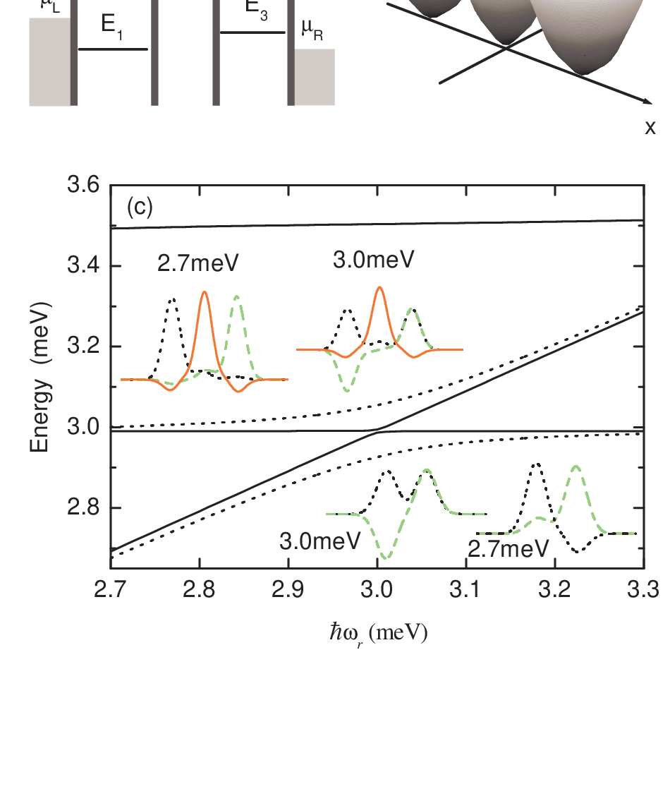
where . In our calculation, the material parameter of GaAs QDs is used as and the value of is taken to resemble experimental systems. We use the eigenstates for each dot as the basis of the Hilbert space. Considering the nonorthogonality of the basis states, we obtain the eigenstates of Eq. (2) by solving the generalized eigenvalue of the system. Here, we investigate the levels of the STQDs by varying with constant parameters of meV, meV, and . For such parameters, the tunneling energy between the left and middle dot is about eV. The lowest three energy levels of STQDs form a -type structure as shown in Fig. 2(a) (c). Experimentally, the levels of each dot are tuned by changing the voltage of the corresponding electrode gate. Such change of voltage corresponds to the variation of confining strength of the dot in our model. As the value of increases, the right level increases. When meV, the energies of and anticross. The corresponding eigenwavefunctions are shown in the insert. It is clear that a pair of delocalized bonding and antibonding states are formed, while the other state is localized in the middle quantum dot. When is away from 3.00 meV, the three levels are nearly energies of the ground states of the left, middle and right dots respectively, and the eigenstates are all localized in each quantum dots. The continuous manifolds on the two sides of the Fig. 2(a) correspond to electronic states with chemical potential and and the two side dots are coupled to the leads with the dots-lead hopping rate and .
Using the same method, we investigate the levels of the DQDs by varying with constant parameters of , and . The lowest two energy levels and the corresponding eigenwavefunctions with different values of of DQDs as shown in Fig.2(c). Similarly, when meV, the energies of and anticross and a pair of delocalized bonding and antibonding states are formed. When is away from 3.00 meV, the two levels are nearly energies of the ground states of the left and right dots respectively, and the eigenstates are localized in each quantum dots.
III Photon-assistant transport properties
III.1 Formulism for photon-assistant transport in coupled QDs system
We first construct our formulism based on parallelly coupled DQDs (see Fig.1 ) with an external time-varying field. This system can be described by the following Hamiltonian:
| (3) |
with
| (4) |
| (5) |
| (6) |
() describes the left and right normal metal leads. models the parallel-coupled DQD where () represents the creation (annihilation) operator of the electron with energy in the dot (). denotes the interdot coupling strength, which can be obtained from the calculations of the electronic structure. Under the adiabatic approximation, the external ac electric field can be reflected in the single-electron energies which can be separated into two parts as and for the central conductor. is the time-independent single-electron energies without the ac field, and is a time-dependent part from the ac field, which can be written as . represents the tunneling coupling between the DQD and leads where is the hopping strength between the th QD and the lead. To capture the essential physics of photon-assisted Fano resonance, we consider the simplest case with noninteracting electrons in two single-level QDs.
The current from the lead to the central region can be calculated from standard NGF techniques, and can be expressed in terms of the dot’s Green function as[33, 34, 35]
| (7) |
Here, the Green’s function and the self-energy are all two-dimensional matrices for the DQD system. The bold-faced letters are used to denote matrices. The retarded and lesser Green functions are defined as and , respectively, with the operator .
The total self-energy is , in which and are caused by the lead and the interdot couplings, respectively. Under the wide-band approximation, the retarded self-energy caused by the lead is defined as
where is the linewidth function defined by with being the density of states of the corresponding lead, describing the coupling between the th QD and the lead. The advanced self-energy can be obtained from . The self-energy caused by the interdot coupling is
The lesser self-energy is and
where denotes the Fermi distribution function of electrons in the lead.
The Green’s function of uncoupled DQD without the couplings to the two leads can be easily obtained as
After taking the Fourier transformations, the Dyson equation and Keldysh equation become
| (20) |
and
| (21) |
respectively. With these Green’s functions, the time-dependent current can be expressed as
| (22) |
Then, the average current is
| (23) |
Here we give another formulism suitable for the serially coupled QDs system. Making use of the Floquet decomposition, the physical picture is clearer in this formulism. As seen in Fig. 1, we should have the serially coupled DQD, if we set . In this case, the self-energies are simplified. It can be shown that
| (24) |
where
| (25) |
| (26) |
(N=2) denote the transmission probabilities for electrons from the right lead and from the left lead, respectively. denotes the Fermi function and
| (27) |
is the Fourier coefficients of the retarded Green function, where are the Fourier coefficients of the Floquet state , , () are the real and imaginary parts of quasi energies respectively. This formulism is valid for general N serially coulped QDs system. [32]
III.2 Transport properties of DQDs

In our numerical calculations, we assume and set the energy independent dots-lead hopping rate , the applied voltage , and the ac field magnitude . First we study the transport properties of an asymmetric system by applying different confining potentials to the left and right dots. The average current-frequency curves of serially and parallel DQDs with are shown in Fig.3 (a) and (b) respectively. We find that the current curve has a symmetric Breit-Wigner line shape when the two dots are serial, and the current has an asymmetric Fano line shape when the dots are parallel. Here the Breit-Wigner line shape is a consequence of photon-assistant resonant, i.e., . The new photon-assistant Fano lineshape comes from the interference between photon-modified bound-antibound channels. Then we apply the same confining potentials to the two dots and research the electron transport of a symmetric system. The results with are displayed in Fig.3 (c) and (d). Similarly, we find that a Breit-Wigner resonance appears in the serially DQDs and a Fano resonance occurs in the parallel DQDs. From above discussion, we conclude that the ac electric field can induce the photon-assisted Fano resonances for both symmetrical and asymmetrical parallel configurations of DQDs, but can not induce Fano resonance in the serially DQDs, whether the system is symmetric or not, which means that the energy level of DQDs does not have remarkable impact on the transport properties.
III.3 Transport properties of STQDs
As one observes in the last section that there is no Fano effect in a serially coupled DQD due the lack of apparent interference channels. One may expect that there is also no Fano resonance in a STQD. However, our studies shows the transport in STQD is quite different from that in a DQD, and we will give a quite different story in this section.
Based on the results of electronic structure in section II, we study the transport properties through the system with -type three-level structure ( Fig.2 ) under the action of an ac driving field with a frequency .
In our numerical calculations, we set the applied voltage , and the other parameters we have chosen are the same as the ones for DQDs.

We first study the transport properties of an asymmetric system by applying different confining potentials to the left and right dots. The average current as a function of the driving frequency with is presented in Fig.4 (a). We find the current curve has a symmetric Breit-Wigner line shape around , suggesting that there is a resonance for electrons in the system in this case (). The time evolution of the probabilities for an electron in left, middle, right dot are shown in Fig.4 (b). Here we have performed our calculation in a closed system (i.e.,without interaction with the leads) and have used the initial condition and the resonant condition . Fig. 4(c) shows the time average of the probability distribution of Floquet states, . It is clear that there is a photon assistant mixing between left and middle dot. This photon assistant charge transfer leads to the occurrence of the current resonance phenomenon.
Then we consider the case that the system is symmetric by applying the same confining potential to the two side dots. The average current as a function of the driving frequency with is displayed in Fig.4 (d). We find that the current curve has an asymmetric Fano line shape around and the current amplitude is much larger than that in the asymmetric case. In order to understand the intriguing phenomenon, we did similar calculation of the time evolution of the occupation probabilities for an electron in left, middle, right dot and the time average of probability distribution of Floquet states. As shown in Fig.4 (e) and (f), we find that two delocalized Floquet states ( which is related to bonding and antibonding states ) are formed and another Floquet state is still localized in the middle dot in this case, indicating that the middle dot mediates the super-exchange interaction between the left and right dots. The states behave like “trapping dark state” in atomic system. Though state has a very small occupation probability in the left and right dots, it plays an important role in the occurrence of the Fano-type resonance, which can be presented in the following discussion.

As seen from Eq. (19), three Floquet states form three conducting channels. Due to the interaction with leads, the three states may have different width. In the symmetric situation, the bonding and antibonding Floquet states , have large occupation probability in left and right dots, thus are strongly coupled to the leads. They have wide width and can be viewed as continuous channels. The localized Floquet state has small occupation probability in left and right dots and is weakly coupled to the leads. It has very narrow width and can be viewed as resonant discrete channel. The interference between strongly coupled channels and weakly coupled channel leads to the observed Fano resonance[37]. While in the asymmetric situation, the Floquet state is also effectively coupled to the leads via a photon-assistant mixing between left and middle dot. Thus all three states form strongly coupled channels, so no Fano effect is observed. Here we discuss in detail the interference between different channels. From Eq. (19), one can see that the average current is mainly decided by . The interference effects can be seen from following calculation (here we show term with , as an example)
| (28) |
In Fig.5, we show the phases as the functions of the driving frequency . Here, the phases and are phases of two strongly coupled states and , and is the phase of the weakly coupled state . From Fig.4, we find that has a phase shift that varies from 0 to as the field frequency is moved through the resonance frequency, which provides resonant channel for electrons to transport the system. , are nearly constant and can be assumed to be independent of the driving frequency, which can be considered as background or nonresonant channels. Therefore, the interference between the strongly coupled channels and weakly coupled channel results in the Fano-type resonance. Finally, we would like to point out that the above picture also explains why there is no Fano resonance in a serially coupled double dot. As a matter of fact, in that situation, there are only strongly coupled bonding and antibonding states. Therefore, there is no apparent Fano effect.
In summary, we have studied the transport properties of DQDs and STQDs under the action of an ac electric field. Using a two-dimensional confining potential model in the effective mass frame, the two-level structure and -type three-level structure are obtained through solving the generalized eigenvalue of the system. Based on the level structure and Floquet theory, we investigate the dependence of the ac current on the electronic structure of the system. It is found that the two-level structure does not influence the transport properties of DQDs remarkably. For both symmetric and asymmetric configurations, there is Fano resonance in parallel DQDs and no Fano resonance in serial DQDs. However, it is a different case for STQDs. The -type three-level structure has great impact on electron transport: when the system is asymmetric, the symmetric Breit-Wigner resonance appears due to phonon assistant tunneling; When the system is symmetric, the interesting asymmetric Fano resonance occurs under resonant condition. In this case, quantum interference results in the formation of trapping dark states. These trapping dark states are the delocalized bonding and antibonding states which serve as the continuous channels. Here the middle dot plays a dual role: (1) It mediates the super-exchange interaction between the left and the right dots; (2) The localized state within it serves as the resonant discrete channel. Our work presents the unique quantum interference features of the multiple quantum dots system and is useful for the design of novel nanodevices. In short, for transport in a system with N quantum dots, the situation with N=1, is different from that with N=2 and the case with N=2 is different from that with N=3. We do not expect qualitative difference for system with .
This work is supported in part by the National Natural Science of China under No. 10574017, 10774016 and a grant of the China Academy of Engineering and Physics.
References
- [1] F. H. L. Koppens, J. A. Folk, J. M. Elzerman, R. Hanson, L. H. Willems van Beveren, I. T. Vink, H. P. Tranitz, W. Wegscheider, L. P. Kouwenhoven, and L. M. K. Vandersypen, Science 309, 1346 (2005).
- [2] A. C. Johnson, J. R. Petta, J. M. Taylor, A. Yacoby, M. D. Lukin, C. M. Marcus, M. P. Hanson, and A. C. Gossard, Nature 435, 925 (2005).
- [3] J. M. Taylor, J. R. Petta, A. C. Johnson, A. Yacoby, C. M. Marcus, and M. D. Lukin, Phys. Rev. B 76, 035315 (2007).
- [4] Y. Ji, M. Heiblum, D. Sprinzak, and Hadas Shtrikman, Science (Washington,DC,U.S.) 290, 779 (2000).
- [5] D. Goldhaber-Gordon, J. Göres, M. A. Kastner, Hadas Shtrikman, D. Mahalu, and U. Meirav, Phys. Rev. Lett. 81, 5225 (1998).
- [6] B. R. Bułka, and P. Stefański, Phys. Rev. Lett. 86, 5128 (2001).
- [7] T. Brandes, and F. Renzoni, Phys. Rev. Lett. 85, 4148 (2000).
- [8] W. D. Chu, S. Duan, and J. Zhu, Appl. Phys. Lett. 90, 222102 (2007).
- [9] J. Göres, D. Goldhaber-Gordon, S. Heemeyer, M. A. Kastner, Hadas Shtrikman, D. Mahalu, and U. Meirav, Phys. Rev. B 62, 2188 (2000).
- [10] A. A. Clerk, X. Waintal, and P. W. Brouwer, Phys. Rev. Lett 86, 4636 (2001).
- [11] A. C. Johnson, C. M. Marcus, M. P. Hanson, and A. C. Gossard, Phys. Rev. Lett. 93, 106803 (2004).
- [12] A.W. Holleitner, C.R. Decker, H. Qin, K. Eberl, and R.H. Blick, Phys. Rev. Lett. 87, 256802 (2001).
- [13] A.W. Holleitner, R.H. Blick, A.K. Hüttel, K. Eberl, and J.P. Kotthaus, Science 297, 70 (2002).
- [14] A.W. Holleitner, R.H. Blick, and K. Eberl, Appl. Phys. Lett. 82, 1887 (2003).
- [15] J.C. Chen, A.M. Chang, and M.R. Melloch, Phys. Rev. Lett. 92, 176801 (2004).
- [16] J. Kim, D. V. Melnikov, J. P. Leburton, D. G. Austing, and S. Tarucha, Phys. Rev. B 74, 035307 (2006).
- [17] D. Schröer, A. D. Greentree, L. Gaudreau, K. Eberl, L. C. L. Hollenberg, J. P. Kotthaus, and S. Ludwig, Phys. Rev. B 76, 075306 (2007).
- [18] D. S. Saraga, and D. Loss, Phys. Rev. Lett. 90, 166803 (2003).
- [19] Z. Jiang, Q. Sun, and Y. Wang, Phys. Rev. B 72, 045332 (2005).
- [20] R. Žitko, J. Bonča, A. Ramšak, and T. Rejec, Phys. Rev. B 73, 153307 (2006).
- [21] R. Žitko, and J. Bonča, Phys. Rev. Lett. 98, 047203 (2007).
- [22] Wei-zhong Wang, Phys. Rev. B 76, 115114 (2007).
- [23] M. L. Ladrón de Guevara, and P. A. Orellana, Phys. Rev. B 73, 205303 (2006).
- [24] J. König and Y. Gefen, Phys. Rev. B 65, 045316 (2002).
- [25] M. L. Ladrón de Guevara, F. Claro, and Pedro A. Orellana, Phys. Rev. B 67, 195335 (2003).
- [26] K. Kang and S. Y. Cho, J. Phys.: Condens. Matter 16, 117 (2004).
- [27] Z.-M. Bai, M.-F. Yang, and Y.-C. Chen, J. Phys.: Condens. Matter 16, 2053 (2004).
- [28] B. Dong, I. Djuric, H. L. Cui, and X. L. Lei, J. Phys.: Condens. Matter 16, 4303 (2004).
- [29] R. López, D. Sánchez, M. Lee, M.-S. Choi, P. Simon, and K. Le Hur, Phys. Rev. B 71, 115312 (2005).
- [30] S. Kohler, J. Lehmann, M. Strass, and P. Hänggi, Adv. Solid State Phys. 44, 157 (2004).
- [31] J. Lehmann, S. Camalet, S. Kohler, and P. Hänggi, Chem. Phys. Lett. 368, 282 (2003).
- [32] S. Kohler, J. Lehmann, and P. Hänggi, Phys. Rep. 406, 379 (2005).
- [33] Antti-Pekka Jauho, N.S. Wingreen, and Y. Meir, Phys. Rev. B 50, 5528 (1994).
- [34] C.A. Stafford and N.S. Wingreen, Phys. Rev. Lett. 76, 1916 (1996).
- [35] Q.F. Sun, J. Wang, and T.H. Lin, Phys. Rev. B 61, 12643 (2000).
- [36] G. Breit, and E. Wigner, Phys. Rev. 49, 519 (1936).
- [37] H. Lu, R. Lu and B. F. Zhu, Phys. Rev. B 71, 235320 (2005).