Chip-Firing and Rotor-Routing
on Directed Graphs

A. E. H. was funded in part by an NSERC discovery grant and Microsoft Research.L. L. was supported by an NSF Graduate Research FellowshipJ. P. was supported by an NSF research grant.2000 Mathematics Subject Classification. Primary: 82C20; secondary: 20K01, 05C25.

Alexander E. Holroyd Address: Department of Mathematics
University of British Columbia Email: holroyd(at)math.ubc.ca Lionel Levine Address: Department of Mathematics
University of California, Berkeley Email: levine(at)math.berkeley.edu Karola Mészáros Address: Department of Mathematics
Massachusetts Institute of Technology Email: karola(at)math.mit.edu Yuval Peres Address: Theory Group
Microsoft Research Email: peres(at)microsoft.com James Propp Address: Department of Mathematical Sciences
University of Massachusetts at Lowell Email: propp(at)cs.uml.edu David B. Wilson Address: Theory Group
Microsoft Research Email: dbwilson(at)microsoft.com

January 16, 2008 (revised May 9, 2013)

Abstract

We give a rigorous and self-contained survey of the abelian sandpile model and rotor-router model on finite directed graphs, highlighting the connections between them. We present several intriguing open problems.

1 Introduction

The abelian sandpile and rotor-router models were discovered several times by researchers in different communities operating independently. The abelian sandpile model was invented by Dhar [Dha90] as a test-bed for the concept of self-organized criticality introduced in [BTW87]. Related ideas were explored earlier by Engel [Eng75, Eng76] in the form of a pedagogical tool (the “probabilistic abacus”), by Spencer [Spe87, pp. 32–35], and by Lorenzini [Lor89, Lor91] in connection with arithmetic geometry. The rotor-router model was first introduced by Priezzhev et al. [PDDK96] (under the name “Eulerian walkers model”) in connection with self-organized criticality. It was rediscovered several times: by Rabani, Sinclair and Wanka [RSW98] as an approach to load-balancing in multiprocessor systems, by Propp [Pro01] as a way to derandomize models such as internal diffusion-limited aggregation (IDLA) [DF91, LBG92], and by Dumitriu, Tetali, and Winkler as part of their analysis of a graph-based game [DTW03]. Articles on the chip-firing game in the mathematical literature include [Big99, Big97, BLS91, BL92]. Those on the rotor-router model include [Lev02, LP05, HP08, LP07a, LP07b]. Below we briefly describe the two models, deferring the formal definitions to later sections.

The abelian sandpile model on a directed graph $G$ , also called the chip-firing game, starts with a collection of chips at each vertex of $G$ . If a vertex $v$ has at least as many chips as outgoing edges, it can fire, sending one chip along each outgoing edge to a neighboring vertex. After firing a sequence of vertices in turn, the process stops when each vertex with positive out-degree has fewer chips than out-going edges. The order of firings does not affect the final configuration, a fact we shall discuss in more detail in Section 2.

To define the rotor-router model on a directed graph $G$ , for each vertex of $G$ , fix a cyclic ordering of the outgoing edges. To each vertex $v$ we associate a rotor $\rho(v)$ chosen from among the outgoing edges from $v$ . A chip performs a walk on $G$ according to the rotor-router rule: if the chip is at $v$ , we first increment the rotor $\rho(v)$ to its successor $e=(v,w)$ in the cyclic ordering of outgoing edges from $v$ , and then route the chip along $e$ to $w$ . If the chip ever reaches a sink, i.e. a vertex of $G$ with no outgoing edges, the chip will stop there; otherwise, the chip continues walking forever.

A common generalization of the rotor-router and chip-firing models, the height arrow model, was proposed in [PDDK96] and studied in [DR04].

We develop the basic theory of the abelian sandpile model in section 2 and define the main algebraic object associated with it, the sandpile group of $G$ [Dha90] (also called the “critical group” by some authors, e.g. [Big99, Wag00]). Furthermore, we establish the basic results about recurrent chip configurations, which play an important role in the theory. In Section 3 we define a notion of recurrent configurations for the rotor-router model on directed graphs and give a characterization for them in terms of oriented spanning trees of $G$ . The sandpile group acts naturally on recurrent rotor configurations, and this action is both transitive and free. We deduce appealing proofs of two basic results of algebraic graph theory, namely the Matrix-Tree Theorem [Sta99, 5.6.8] and the enumeration of Eulerian tours in terms of oriented spanning trees [Sta99, Cor. 5.6.7]. We also derive a family of bijections between the recurrent chip configurations of $G$ and the recurrent rotor configurations of $G$ . Such bijections have been constructed before, for example in [BW97]; however, our presentation differs significantly from the previous ones. Section 4 establishes stronger results for both models on Eulerian digraphs and undirected graphs. In Section 5 we present an alternative view of the rotor-router model in terms of “cycle-popping,” borrowing an idea from Wilson’s work on loop-erased random walk; see [PW98]. We conclude in Section 6 by presenting some open questions.

2 Chip-Firing

In a finite directed graph (digraph) $G=(V,E)$ , a directed edge $e\in E$ points from the vertex ${\rm tail}(e)$ to the vertex ${\rm head}(e)$ . We allow self-loops ( ${\rm head}(e)={\rm tail}(e)$ ) as well as multiple edges ( ${\rm head}(e)={\rm head}(e^{\prime})$ and ${\rm tail}(e)={\rm tail}(e^{\prime})$ ) in $G$ . The out-degree $\operatorname{outdeg}(v)$ of a vertex $v$ (also denoted by $d_{v}$ ) is the number of edges $e$ with ${\rm tail}(e)=v$ , and the in-degree $\operatorname{indeg}(v)$ of $v$ is the number of edges $e$ with ${\rm head}(e)=v$ . A vertex is a sink if its out-degree is zero. A global sink is a sink $s$ such that from every other vertex there is a directed path leading to $s$ . Note that if there is a global sink, then it is the unique sink.

If $G$ has the same number of edges from $v$ to $w$ as from $w$ to $v$ for all vertices $v\neq w$ then we call $G$ bidirected. In particular, a bidirected graph is obtained by replacing each edge of an undirected graph with a pair of directed edges, one in each direction.

Label the vertices of $G$ as $v_{1},v_{2},\dots,v_{n}$ . The adjacency matrix $A$ of $G$ is the $n\times n$ matrix whose $(i,j)$ -entry is the number of edges from $v_{i}$ to $v_{j}$ , which we denote by $a_{v_{i},v_{j}}$ or $a_{ij}$ . The (graph) Laplacian of $G$ is the $n\times n$ matrix $\Delta=D-A$ , where $D$ is the diagonal matrix whose $(i,i)$ -entry is the out-degree of $v_{i}$ , which we denote by $d_{v_{i}}$ or $d_{i}$ . That is,

\Delta_{ij}=\begin{cases}-a_{ij}&\text{for $i\neq j$,}\\ d_{i}-a_{ii}&\text{for $i=j$.}\end{cases}

Note that the entries in each row of $\Delta$ sum to zero. If the vertex $v_{i}$ is a sink, then the $i$ ${}^{\text{th}}$ row of $\Delta$ is zero.

A chip configuration $\sigma$ on $G$ , also called a sandpile on $G$ , is a vector of non-negative integers indexed by the non-sink vertices of $G$ , where $\sigma(v)$ represents the number of chips at vertex $v$ . A chip configuration $\sigma$ is stable if $\sigma(v)<d_{v}$ for every non-sink vertex $v$ . We call a vertex $v$ active in $\sigma$ if $v$ is not a sink and $\sigma(v)\geq d_{v}$ . An active vertex $v$ can fire, resulting in a new chip configuration $\sigma^{\prime}$ obtained by moving one chip along each of the $d_{v}$ edges emanating from $v$ ; that is, $\sigma^{\prime}(w)=\sigma(w)+a_{vw}$ for all $w\neq v$ and $\sigma^{\prime}(v)=\sigma(v)-d_{v}+a_{vv}$ . We call the configuration $\sigma^{\prime}$ a successor of $\sigma$ .

By performing a sequence of firings, we may eventually arrive at a stable chip configuration, or we might continue firing forever, as the following examples show.

Example 2.1.

Consider the complete directed graph on three vertices (without self-loops). Then placing three chips at a vertex gives a configuration that stabilizes in one move, while placing four chips at a vertex gives a configuration that never stabilizes (see Figure 1).

Refer to caption — Figure 1: Some chip configurations eventually stabilize, while others never stabilize.

It might appear that the choice of the order in which we fire vertices could affect the long-term behavior of the system; however, this is not the case, as the following lemma shows (and Figure 2 illustrates).

Lemma 2.2 ([Dha90],[DF91]).

Let $G$ be any digraph, let $\sigma_{0}$ , $\sigma_{1},\ldots,\sigma_{n}$ be a sequence of chip configurations on $G$ , each of which is a successor of the one before, and let $\sigma^{\prime}_{0},\sigma^{\prime}_{1},\ldots,\sigma^{\prime}_{m}$ be another such sequence with $\sigma^{\prime}_{0}=\sigma_{0}$ .

1.

If $\sigma_{n}$ is stable, then $m\leq n$ , and moreover, no vertex fires more times in $\sigma^{\prime}_{0},\ldots,\sigma^{\prime}_{m}$ than in $\sigma_{0},\ldots,\sigma_{n}$ .
2.

If $\sigma_{n}$ and $\sigma^{\prime}_{m}$ are both stable, then $m=n$ , $\sigma_{n}=\sigma^{\prime}_{n}$ , and each vertex fires the same number of times in both histories.

Proof.

Part 2 is an immediate corollary of part 1, which we now prove. If part 1 fails, then consider a counterexample with $m+n$ minimal. Let $v_{i}$ be the vertex that fires when $\sigma_{i-1}$ becomes $\sigma_{i}$ , and $v^{\prime}_{i}$ be the vertex that fires when $\sigma^{\prime}_{i-1}$ becomes $\sigma^{\prime}_{i}$ . Vertex $v^{\prime}_{1}$ must be fired at some stage (say the $i$ ${}^{\text{th}}$ ) in the sequence of configurations $\sigma_{0},\dots,\sigma_{n}$ , since $\sigma_{n}$ is stable; say $v_{i}$ = $v^{\prime}_{1}$ . Then $v_{i},v_{1},v_{2},\dots,v_{i-1},v_{i+1},\dots,v_{n}$ is a permissible firing sequence that turns $\sigma_{0}$ into $\sigma_{n}$ with the same number of firings at each site as the unpermuted sequence. The firing sequences $v_{1},\dots,v_{i-1},v_{i+1},\\ \dots,v_{n}$ and $v^{\prime}_{2},v^{\prime}_{3},\dots,v^{\prime}_{m}$ then constitute a smaller counterexample to the lemma (with initial configuration $\sigma^{\prime}_{1}$ ), contradicting minimality. ∎

Definition 2.3.

Starting from a configuration $\sigma$ , Lemma 2.2 shows that there is at most one stable configuration that can be reached by a finite sequence of firings (and that if such a configuration exists, then no infinite sequence of firings is possible). If such a stable configuration exists we denote it $\sigma^{\circ}$ and call it the stabilization of $\sigma$ .

Thus far, the presence or absence of sinks was irrelevant for our claims. For the rest of this section, we assume that the digraph $G$ has a global sink $s$ .

Lemma 2.4.

If digraph $G$ has a global sink, then every chip configuration on $G$ stabilizes.

Proof.

Let $N$ be the number of chips in the configuration. Given a vertex $v$ of $G$ , let $v_{0},v_{1},\dots,v_{r-1},v_{r}$ be a directed path from $v_{0}=v$ to $v_{r}=s$ . Every time $v_{r-1}$ fires, it sends a chip to the sink which remains there forever. Thus $v_{r-1}$ can fire at most $N$ times. Every time $v_{r-2}$ fires, it sends a chip to $v_{r-1}$ , and $d_{v_{r-1}}$ such chips will cause $v_{r-1}$ to fire once, so $v_{r-2}$ fires at most $d_{v_{r-1}}N$ times. Iterating backward along the path, we see that $v$ fires at most $d_{v_{1}}\cdots d_{v_{r-1}}N$ times. Thus each vertex can fire only finitely many times, so by Lemma 2.2 the configuration stabilizes. ∎

We remark that when $G$ is connected and the sink is the only vertex with in-degree exceeding its out-degree, the bound one gets from the above argument on the total number of firings is far from optimal; see Proposition 4.8 for a better bound.

Define the chip addition operator $E_{v}$ as the map on chip configurations that adds a single chip at vertex $v$ and then lets the system stabilize. In symbols,

E_{v}\sigma=(\sigma+{\mathbf{1}}_{v})^{\circ}

where ${\mathbf{1}}_{v}$ is the configuration consisting of a single chip at $v$ .

Lemma 2.5.

On any digraph with a global sink, the chip addition operators commute.

Proof.

Given a chip configuration $\sigma$ and two vertices $v$ and $w$ , whatever vertices are active in $\sigma+{\mathbf{1}}_{v}$ are also active in configuration $\sigma^{\prime}=\sigma+{\mathbf{1}}_{v}+{\mathbf{1}}_{w}$ . Applying to $\sigma^{\prime}$ a sequence of firings that stabilizes $\sigma+{\mathbf{1}}_{v}$ , we obtain the configuration $E_{v}\sigma+{\mathbf{1}}_{w}$ . Stabilizing this latter configuration yields $E_{w}E_{v}\sigma$ . Thus $E_{w}E_{v}\sigma$ is a stabilization of $\sigma^{\prime}$ . Interchanging the roles of $v$ and $w$ , the configuration $E_{v}E_{w}\sigma$ is also a stabilization of $\sigma^{\prime}$ . From Lemma 2.2 we conclude that $E_{w}E_{v}\sigma=E_{v}E_{w}\sigma$ . ∎

Lemma 2.5 is called the abelian property; it justifies Dhar’s coinage “abelian sandpile model”. From the above proof we also deduce the following.

Corollary 2.6.

Applying a sequence of chip addition operators to $\sigma$ yields the same result as adding all the associated chips simultaneously and then stabilizing.

Let $G$ be a digraph on $n$ vertices with global sink $s$ . The reduced Laplacian $\Delta^{\prime}$ of $G$ is obtained by deleting from the Laplacian matrix $\Delta$ the row and column corresponding to the sink. Note that firing a non-sink vertex $v$ transforms a chip configuration $\sigma$ into the configuration $\sigma-\Delta^{\prime}_{v}$ , where $\Delta^{\prime}_{v}$ is the row of the reduced Laplacian corresponding to $v$ . Since we want to view the configurations before and after firing as equivalent, we are led to consider the group quotient ${\mathbb{Z}}^{n-1}/H$ , where $H={\mathbb{Z}}^{n-1}\Delta^{\prime}$ is the integer row-span of $\Delta^{\prime}$ .

Definition 2.7.

Let $G$ be a digraph on $n$ vertices with global sink $s$ . The sandpile group of $G$ is the group quotient

\mathcal{S}(G)={\mathbb{Z}}^{n-1}/{\mathbb{Z}}^{n-1}\Delta^{\prime}(G).

The connection between the sandpile group and the dynamics of sandpiles on $G$ is made explicit in Corollary 2.16. For the graph in Figure 3, the sandpile group is the cyclic group of order 3. The group structure of $\mathcal{S}(G)$ when $G$ is a tree is investigated in [Lev07].

Lemma 2.8.

The order of $\mathcal{S}(G)$ is the determinant of the reduced Laplacian $\Delta^{\prime}(G)$ .

Proof.

The order of $\mathcal{S}(G)$ equals the index of the lattice $H={\mathbb{Z}}^{n-1}\Delta^{\prime}$ in ${\mathbb{Z}}^{n-1}$ , and, recalling that the volume of a parallelepiped is the determinant of the matrix formed from its edge-vectors, we deduce that this in turn equals the determinant of $\Delta^{\prime}$ . ∎

Lemma 2.9.

Let $G$ be a digraph with a global sink. Every equivalence class of ${\mathbb{Z}}^{n-1}$ modulo $\Delta^{\prime}(G)$ contains at least one stable chip configuration of $G$ .

Proof.

Let ${\mathbf{\delta}}$ be the configuration given by ${\mathbf{\delta}}(v)=d_{v}$ for all $v$ , and let ${\mathbf{\delta}}^{\circ}$ be its stabilization. Then ${\mathbf{\delta}}^{\circ}(v)<d_{v}$ for all $v\neq s$ , so ${\mathbf{\delta}}-{\mathbf{\delta}}^{\circ}$ is a positive vector equivalent to the zero configuration. Given any $\alpha\in{\mathbb{Z}}^{n-1}$ , let $m$ denote the minimum of all the coordinates of $\alpha$ together with 0 (so that $m\leq 0$ ). Then the vector

\beta=\alpha+(-m)({\mathbf{\delta}}-{\mathbf{\delta}}^{\circ})

is nonnegative and equivalent to $\alpha$ . Hence $\beta^{\circ}$ is a stable chip configuration in the same equivalence class as $\alpha$ . ∎

Example 2.10.

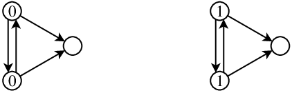
An equivalence class may contain more than one stable chip configuration. For example, consider the complete directed graph on three vertices, with one of the vertices made into a sink by deletion of its two outgoing edges (see Figure 3). It is easy to see that there are two stable configurations in the equivalence class of the identity: the configuration in which each of the two non-sink vertices has 0 chips and the configuration in which each of the two vertices has 1 chip. It might seem natural that, if either of these two configurations is to be preferred as a representative of the identity element in the sandpile group, it should be the former. However, this instinct is misleading, as we now explain.

Definition 2.11.

A chip configuration $\sigma$ is accessible if from any other chip configuration it is possible to obtain $\sigma$ by a combination of adding chips and selectively firing active vertices. A chip configuration that is both stable and accessible is called recurrent.

Remark 2.12.

There are several definitions of “recurrent” that are used in the literature. Lemma 2.17 below shows that these definitions (including the one above) are equivalent for any digraph with a global sink.

We will see shortly (in Lemmas 2.13 and 2.15) that each equivalence class in ${\mathbb{Z}}^{n-1}/{\mathbb{Z}}^{n-1}\Delta^{\prime}$ contains a unique recurrent chip configuration. It is customary to represent each element of the sandpile group by its unique recurrent element. In Example 2.10 the all-1 configuration is accessible, but the all-0 configuration is not. Therefore the all-1 configuration is taken as the canonical representative of the identity. (However, in the context of cluster-firing and superstabilization as described in Definition 4.3 and Lemma 4.6, the all-0 configuration will be the preferred representative.)

Lemma 2.13.

Let $G$ be a digraph with a global sink. Every equivalence class of ${\mathbb{Z}}^{n-1}$ modulo $\Delta^{\prime}(G)$ contains at least one recurrent chip configuration of $G$ .

Proof.

Given $\alpha\in{\mathbb{Z}}^{n-1}$ , let $m$ denote the minimum of all the coordinates of $\alpha$ together with 0, so that $m\leq 0$ . Write $d_{\max}$ for the maximum out-degree of a vertex in $G$ . Then $\alpha$ is equivalent to the configuration

\beta=\alpha+[d_{\max}+(-m)]({\mathbf{\delta}}-{\mathbf{\delta}}^{\circ})

with ${\mathbf{\delta}}$ as in the proof of Lemma 2.9. Since ${\mathbf{\delta}}-{\mathbf{\delta}}^{\circ}$ has all entries positive, we have $\alpha\geq m(\delta-\delta^{\circ})$ and hence $\beta\geq d_{\max}$ . (Inequalities between two vectors or between a vector and a scalar are interpreted componentwise.) In particular, $\beta$ is accessible, since any chip configuration can first be stabilized, so that each vertex has fewer than $d_{\max}$ chips, and then supplemented with extra chips to obtain $\beta$ . Therefore any configuration obtained from $\beta$ by firing is also accessible. In particular the stabilization $\beta^{\circ}$ is thus recurrent and equivalent to $\alpha$ . ∎

Next we will show that every equivalence class modulo $\Delta^{\prime}$ contains at most one recurrent configuration, making use of the following lemma.

Lemma 2.14.

Let $\epsilon=(2\delta)-(2\delta)^{\circ}$ , where $\delta$ is given by $\delta(v)=d_{v}$ as before. If $\sigma$ is recurrent, then $(\sigma+\epsilon)^{\circ}=\sigma$ .

Proof.

If $\sigma$ is recurrent then it is accessible, so it can be reached from $\delta$ by adding some (non-negative) configuration $\zeta$ and selectively firing. But since $\sigma$ is also stable this implies that $(\zeta+\delta)^{\circ}=\sigma$ . Consider the configuration

\gamma=(\zeta+\delta)+\epsilon=2\delta+\zeta+\delta-(2\delta)^{\circ}.

Since $\epsilon\geq 0$ , we may start from $\gamma$ and fire a sequence of vertices that stabilizes $\zeta+\delta$ , to obtain the configuration $\sigma+\epsilon$ . On the other hand, since $\delta-(2\delta)^{\circ}\geq 0$ we may start from $\gamma$ and fire a sequence of vertices that stabilizes $2\delta$ , to obtain the configuration $(2\delta)^{\circ}+\zeta+\delta-(2\delta)^{\circ}=\zeta+\delta$ , which in turn stabilizes to $\sigma$ . By Lemma 2.2 it follows that $(\sigma+\epsilon)^{\circ}=\sigma$ . ∎

Lemma 2.15.

Let $G$ be a digraph with a global sink. Every equivalence class of ${\mathbb{Z}}^{n-1}$ modulo $\Delta^{\prime}(G)$ contains at most one recurrent chip configuration of $G$ .

Proof.

Let $\sigma_{1}$ and $\sigma_{2}$ be recurrent and equivalent mod $\Delta^{\prime}$ . Label the non-sink vertices $v_{1},\ldots,v_{n-1}$ . Then $\sigma_{1}=\sigma_{2}+\sum_{i\in J}c_{i}\Delta^{\prime}_{i}$ , where the $c_{i}$ are nonzero constants, $\Delta^{\prime}_{i}$ is the row of the reduced Laplacian $\Delta^{\prime}$ corresponding to $v_{i}$ , and the index $i$ runs over some subset $J$ of the integers $1,\ldots,n-1$ . Write $J=J_{-}\cup J_{+}$ , where $J_{-}=\{i:c_{i}<0\}$ and $J_{+}=\{i:c_{i}>0\}$ , and let

\sigma=\sigma_{1}+\sum_{i\in J_{-}}(-c_{i})\Delta^{\prime}_{i}=\sigma_{2}+\sum_{i\in J_{+}}c_{i}\Delta^{\prime}_{i}.

Let $\epsilon$ denote the everywhere-positive chip configuration defined in Lemma 2.14. Take $k$ large enough so that $\sigma^{\prime}=\sigma+k\epsilon$ satisfies $\sigma^{\prime}(v_{i})\geq|c_{i}|d_{v_{i}}$ for all $i$ . Starting from $\sigma^{\prime}$ , we may fire each vertex $v_{i}$ for $i\in J_{-}$ a total of $-c_{i}$ times, and each of the intermediate configurations is a valid chip configuration because all the entries are nonnegative. The resulting configuration $\sigma_{1}+k\epsilon$ then stabilizes to $\sigma_{1}$ by Lemma 2.14. Likewise, starting from $\sigma^{\prime}$ we may fire each vertex $v_{i}$ for $i\in J_{+}$ a total of $c_{i}$ times to obtain $\sigma_{2}+k\epsilon$ , which stabilizes to $\sigma_{2}$ . By Lemma 2.2 it follows that $\sigma_{1}=\sigma_{2}$ . ∎

Corollary 2.16.

Let $G$ be a digraph with a global sink. The set of all recurrent chip configurations on $G$ is an abelian group under the operation $(\sigma,\sigma^{\prime})\mapsto(\sigma+\sigma^{\prime})^{\circ}$ , and it is isomorphic via the inclusion map to the sandpile group $\mathcal{S}(G)$ .

Proof.

Immediate from Lemmas 2.13 and 2.15. ∎

In view of this isomorphism, we will henceforth use the term “sandpile group” to refer to the group of recurrent configurations.

It is of interest to consider the identity element $I$ of the sandpile group, i.e. the unique recurrent configuration equivalent to the all-0 configuration. Here is one method to compute $I$ . Let $\sigma$ be the configuration $2\delta-2$ . (Arithmetic combinations of vectors and scalars are to interpreted componentwise.) Since $\sigma^{\circ}\leq\delta-1$ we have $\sigma-\sigma^{\circ}\geq\delta-1$ , so $\sigma-\sigma^{\circ}$ is accessible. Since $\sigma-\sigma^{\circ}$ is equivalent to 0, the identity element is given by $I=(\sigma-\sigma^{\circ})^{\circ}$ .

Figure 4 shows identity elements for the $L\times L$ square grid with “wired boundary,” for several values of $L$ . (To be more precise, the graph $G$ is obtained by replacing each edge of the undirected square grid with a pair of directed edges, and adjoining a sink vertex $s$ along with two edges from each of the four corner vertices to $s$ and one edge from each of the other boundary vertices to $s$ .) The identity element of this graph was studied by Le Borgne and Rossin [BR02], but most basic properties of this configuration, such as the existence of the large square in the center, remain unproved.

Figure 5 shows another example, the identity element for the $100\times 100$ directed torus. (That is, for each vertex $(i,j)\in{\mathbb{Z}}/100{\mathbb{Z}}\times{\mathbb{Z}}/100{\mathbb{Z}}$ , there are directed edges from $(i,j)$ to $(i+1\bmod 100,j)$ and to $(i,j+1\bmod 100)$ , and we make $(0,0)$ (the lower-left vertex) into a sink by deleting its two outgoing edges.)

Figure 6 shows a third example, the identity element for a disk-shaped region of ${\mathbb{Z}}^{2}$ with wired boundary. Examples of identity elements for graphs formed from portions of lattices other than the square grid can be found in [LKG90].

Also of interest is the inverse of a recurrent chip configuration $\sigma$ (that is, the recurrent chip configuration $\bar{\sigma}$ such that $(\sigma+\bar{\sigma})^{\circ}=I$ ). One way to compute the inverse is via $\bar{\sigma}=(\zeta-\zeta^{\circ}-\sigma)^{\circ}$ , where $\zeta$ is any chip configuration satisfying $\zeta\geq 3\delta-3$ . (Here $\zeta-\zeta^{\circ}-\sigma$ is accessible, since it has at least $d_{v}-1$ chips at each vertex $v$ .)

Given two chip configurations $\sigma$ and $\zeta$ , we say that $\sigma$ is reachable from $\zeta$ (via excitation-relaxation operations) if there exists a configuration $\beta$ such that $\sigma=(\zeta+\beta)^{\circ}$ . Note that this implies that $\sigma$ is stable. A digraph is strongly connected if for any two distinct vertices $v,w$ there are directed paths from $v$ to $w$ and from $w$ to $v$ . We write $G\smallsetminus s$ for the graph obtained from $G$ by deleting the vertex $s$ along with all edges incident to $s$ .

Lemma 2.17.

Let $G$ be a digraph with a global sink $s$ , and let $\sigma$ be a chip configuration on $G$ . The following are equivalent.

(1)

$\sigma$ is recurrent; that is, $\sigma$ is reachable from any configuration $\zeta$ .
(2)

If $\zeta$ is any configuration reachable from $\sigma$ , then $\sigma$ is reachable from $\zeta$ .
(3)

$\sigma$ is reachable from any configuration of the form $E_{v}\sigma$ , where $v$ is a non-sink vertex of $G$ .
(4)

Each strongly connected component of $G\smallsetminus s$ contains a vertex $v$ such that $\sigma$ is reachable from $E_{v}\sigma$ .

Proof.

Since trivially $(1)\Rightarrow(2)\Rightarrow(3)\Rightarrow(4)$ , it suffices to show $(4)\Rightarrow(1)$ .

If (4) holds, there is a chip configuration $\alpha$ such that $(\sigma+\alpha)^{\circ}=\sigma$ and $\alpha$ is nonzero on at least one vertex of each strongly connected component of $G$ . There exists a positive integer $k$ such that selective firing from $k\alpha$ results in a chip configuration $\beta$ with at least one chip at each vertex. Moreover, $(\sigma+\beta)^{\circ}=\sigma$ .

Now let $\zeta$ be any chip configuration. Since $\beta$ has at least one chip at each vertex, we have $\zeta\leq\sigma+\ell\beta$ for some integer $\ell$ . Thus we may add chips to $\zeta$ and then stabilize to obtain the configuration $(\sigma+\ell\beta)^{\circ}=\sigma$ . Hence $\sigma$ is recurrent. ∎

We also note that, for a digraph $G$ with a global sink, the sandpile group is isomorphic to the additive group of harmonic functions modulo 1 on $G$ that vanish on the sink [Sol99]. A function $f:V(G)\to[0,1)$ is harmonic modulo 1 if $d_{v}f(v)=\sum_{w}a_{v,w}f(w)\mod 1$ for all vertices $v$ . For a sandpile configuration $\sigma$ , the associated harmonic function $f$ is the fractional part of the solution $\tilde{f}$ of

\sum_{w}\Delta^{\prime}_{v,w}\tilde{f}(w)=\sigma(v).

For the graph in Figure 3, the three harmonic functions are $(f(v_{1}),f(v_{2}))=(0,0)$ , $(f(v_{1}),f(v_{2}))=(1/3,2/3)$ , and $(f(v_{1}),f(v_{2}))=(2/3,1/3)$ .

We conclude this section by pointing out a link between the sandpile group and spanning trees. By Lemma 2.8 the order of the sandpile group of $G$ equals the determinant of the reduced Laplacian $\Delta^{\prime}$ of $G$ . By the matrix-tree theorem [Sta99, 5.6.8], this determinant equals the number of oriented spanning trees of $G$ rooted at the sink (that is, acyclic subgraphs of $G$ in which every non-sink vertex has out-degree 1). Various bijections have been given for this correspondence; see, for example, [BW97]. In Section 3 we will use the rotor-router model to describe a particularly natural bijection, and deduce the matrix-tree theorem as a corollary.

3 Rotor-Routing

Chip-firing is a way of routing chips through a directed graph $G$ in such a fashion that the chips emitted by any vertex $v$ travel in equal numbers along each of the outgoing edges. In order to ensure this equality, however, chips must wait at a vertex $v$ until sufficiently many additional chips have arrived to render $v$ active. Rotor-routing is an alternative approach to distributing chips through $G$ which dispenses with this waiting step. Since we cannot ensure exact equality without waiting, we settle for the condition that the chips emitted by any vertex $v$ travel in nearly equal numbers along each of the edges emanating from $v$ . We ensure that this near-equality holds by using a rotor mechanism to decide where each successive chip emitted from a vertex $v$ should be routed.

Given a directed graph $G$ , fix for each vertex $v$ a cyclic ordering of the edges emanating from $v$ . For an edge $e$ with tail $v$ we denote by $e^{+}$ the next edge after $e$ in the prescribed cyclic ordering of the edges emanating from $v$ .

Definition 3.1.

A rotor configuration is a function $\rho$ that assigns to each non-sink vertex $v$ of $G$ an edge $\rho(v)$ emanating from $v$ . If there is a chip at a non-sink vertex $v$ of $G$ , routing the chip at $v$ (for one step) consists of updating the rotor configuration so that $\rho(v)$ is replaced with $\rho(v)^{+}$ , and then moving the chip to the head of $\rho(v)^{+}$ . A single-chip-and-rotor state is a pair consisting of a vertex $w$ (which represents the location of the chip) and a rotor configuration $\rho$ . The rotor-router operation is the map that sends a single-chip-and-rotor state $(w,\rho)$ (where $w$ is not a sink) to the state $(w^{+},\rho^{+})$ obtained by routing the chip at $w$ for one step. (See Figure 7 for examples of the rotor-router operation.)

As we will see, there is an important link between chip-firing and rotor-routing. A hint at this link comes from a straightforward count of configurations. Recall that a stable chip configuration is a way of assigning some number of chips between 0 and $d_{v}-1$ to each non-sink vertex $v$ of $G$ . Thus, the number of stable configurations is exactly $\prod_{v}d_{v}$ , where the product runs over all non-sink vertices. This is also the number of rotor configurations on $G$ . Other connections become apparent when one explores the appropriate notion of recurrent states for the rotor-router model. We will treat two cases separately: digraphs with no sink, and digraphs with a global sink (Lemma 3.6 applies to both settings).

Definition 3.2.

Let $G$ be a sink-free digraph, i.e. one in which each vertex has at least one outgoing edge. Starting from the state $(w,\rho)$ , if iterating the rotor-router operation eventually leads back to $(w,\rho)$ we say that $(w,\rho)$ is recurrent; otherwise, it is transient.

Our first goal is to give a combinatorial characterization of the recurrent states, Theorem 3.8. We define a unicycle to be a single-chip-and-rotor state $(w,\rho)$ for which the set of edges $\{\rho(v)\}$ contains a unique directed cycle, and $w$ lies on this cycle. (Equivalently, $\rho$ is a connected functional digraph, and $w$ is a vertex on the unique cycle in $\rho$ .) The following lemma shows that the rotor-router operation takes unicycles to unicycles.

Lemma 3.3.

Let $G$ be a sink-free digraph. If $(w,\rho)$ is a unicycle on $G$ , then $(w^{+},\rho^{+})$ is also a unicycle.

Proof.

Since $(w,\rho)$ is a unicycle, the set of edges $\{\rho(v)\}_{v\neq w}=\{\rho^{+}(v)\}_{v\neq w}$ contains no directed cycles. The set of edges $\{\rho^{+}(v)\}$ forms a subgraph of $G$ in which every vertex has out-degree one, so it contains a directed cycle. Since any such cycle must contain the edge $\rho^{+}(w)=\rho(w)^{+}$ , this cycle is unique, and $w^{+}$ lies on it. ∎

Lemma 3.4.

Let $G$ be a sink-free digraph. The rotor-router operation is a permutation on the set of unicycles of $G$ .

Proof.

Since the set of unicycles is finite, by Lemma 3.3 it is enough to show surjectivity. Given a unicycle $U=(w,\rho)$ , let $U^{-}=(w^{-},\rho^{-})$ be the state obtained by moving the chip from $w$ to its predecessor $w^{-}$ in the unique cycle through $w$ , and replacing the rotor at $w^{-}$ with its predecessor in the cyclic ordering of outgoing edges from $w^{-}$ . Then the rotor-router operation applied to $U^{-}$ yields $U$ . It remains to show that $U^{-}$ is a unicycle; for this it suffices to show that every directed cycle in $\rho^{-}$ passes through $w^{-}$ . Suppose that there is a directed cycle of rotors in $\rho^{-}$ which avoids $w^{-}$ . Since $\rho^{-}$ agrees with $\rho$ except at $w^{-}$ , this same directed cycle occurs within $\rho$ and avoids $w^{-}$ , a contradiction since $w^{-}$ is on $\rho$ ’s unique cycle. ∎

Corollary 3.5.

Let $G$ be a sink-free digraph. If $(w,\rho)$ is a unicycle on $G$ , then $(w,\rho)$ is recurrent.

In Lemma 3.7, below, we show that the converse holds when $G$ is strongly connected. We will need the following lemma, which is analogous to Lemma 2.4 for the abelian sandpile. A vertex $w$ is globally reachable if for each other vertex $v$ there is a directed path from $v$ to $w$ .

Lemma 3.6.

Let $G$ be a digraph with a globally reachable vertex $w$ . For any starting vertex and rotor configuration, iterating the rotor-router operation a suitable number of times yields a state in which the chip is at $w$ .

Proof.

Since $w$ is globally reachable, either $G$ is sink-free or $w$ is the unique sink. Thus either we can iterate the rotor-router operation indefinitely, or the chip eventually visits $w$ . In the former case, since $G$ is finite, the chip visits some vertex $v$ infinitely often. But if $x$ is a vertex that is visited infinitely often and there is an edge from $x$ to $y$ , then $y$ is also visited infinitely often. Inducting along a path from $v$ to $w$ , we conclude that the chip eventually visits $w$ . ∎

Lemma 3.7.

Let $G$ be a strongly connected digraph. If $(w,\rho)$ is a recurrent single-chip-and-rotor state on $G$ , then it is a unicycle.

Proof.

Since $G$ is strongly connected, every vertex is globally reachable. Hence by Lemma 3.6, if we start from any initial state and iterate the rotor-router rule sufficiently many times, the chip visits every vertex of $G$ .

Suppose $(w,\rho)$ is a recurrent state. Once every vertex has been visited and we return to the state $(w,\rho)$ , suppose the rotors at vertices $v_{1}\ldots,v_{k}$ form a directed cycle. If $w$ does not lie on this cycle, then for each $i$ , the last time the chip was at $v_{i}$ it moved to $v_{i+1}$ , and hence the edge from $v_{i}$ to $v_{i+1}$ was traversed more recently than the edge from $v_{i-1}$ to $v_{i}$ . Carrying this argument around the cycle leads to a contradiction. Thus, every directed cycle in the rotor configuration must pass through $w$ . But now if we start from $w$ and follow the rotors, the first vertex we revisit must be $w$ . Hence $(w,\rho)$ is a unicycle. ∎

Combining Corollary 3.5 and Lemma 3.7, we have proved the following.

Theorem 3.8.

Let $G$ be a strongly connected digraph. Then $(w,\rho)$ is a recurrent single-chip-and-rotor state on $G$ if and only if it is a unicycle.

Next we consider the case when $G$ is a digraph with a global sink. Note that we cannot apply the rotor-router operation to states in which the chip is at the sink. We call these absorbing states. For any starting state, if we iterate the rotor-router operation sufficiently many times, the chip must eventually arrive at the sink by Lemma 3.6.

A chip-and-rotor state is a pair $\tau=(\sigma,\rho)$ consisting of a chip configuration $\sigma$ and rotor configuration $\rho$ on $G$ . A non-sink vertex is active in $\tau$ if it has at least one chip. If $v$ is active, then firing $v$ results in a new chip-and-rotor state given by replacing the rotor $\rho(v)$ with $\rho(v)^{+}$ and moving a single chip from $v$ to the head of $\rho(v)^{+}$ (and removing the chip if $\rho(v)^{+}$ is a sink). We say that $\tau^{\prime}$ is a successor of $\tau$ if it is obtained from $\tau$ by firing an active vertex. We say that $\tau$ is stable if no vertex can fire, i.e., all chips have moved to a sink and disappeared. The rotor-router operation has the following abelian property analogous to Lemma 2.2.

Lemma 3.9.

Let $G$ be a digraph with a global sink. Let $\tau_{0}$ , $\tau_{1},\ldots,\tau_{n}$ be a sequence of chip-and-rotor states of $G$ , each of which is a successor of the one before. If $\tau_{0},\tau^{\prime}_{1},\ldots,\tau^{\prime}_{m}$ is another such sequence, and $\tau_{n}$ is stable, then $m\leq n$ . If in addition $\tau^{\prime}_{m}$ is stable, then $m=n$ and $\tau_{n}=\tau^{\prime}_{n}$ , and for each vertex $w$ , the number of times $w$ fires is the same for both histories.

Proof.

Let $v_{i}$ and $v^{\prime}_{i}$ be the vertices that are fired in $\tau_{i-1}$ and $\tau^{\prime}_{i-1}$ to obtain $\tau_{i}$ and $\tau^{\prime}_{i}$ , respectively. We will show that if $\tau_{n}$ is stable and the sequences $v$ and $v^{\prime}$ agree in the first $i-1$ terms for some $i\leq m$ , then some permutation of $v$ agrees with $v^{\prime}$ in the first $i$ terms. Since $v^{\prime}_{i}$ is active in $\tau_{i-1}=\tau^{\prime}_{i-1}$ , it must be active in $\tau_{i},\tau_{i+1},\dots$ , until it is fired. Since $\tau_{n}$ is stable, it follows that $v_{j}=v^{\prime}_{i}$ for some $j>i$ . Let $j$ be the minimal such index. Starting from $\tau_{0}$ , the vertices $v_{1},v_{2},\ldots,v_{i-1},v_{j},v_{i},v_{i+1},\ldots,v_{j-1},v_{j+1},\ldots,v_{n}$ can be fired in that order, resulting in the same stable configuration $\tau_{n}$ . Moreover, this sequence agrees with $v^{\prime}$ in the first $i$ terms.

By induction, it follows that the sequence $v^{\prime}$ is an initial subsequence of a permutation of $v$ . In particular, $m\leq n$ . If $\tau^{\prime}_{m}$ is also stable, by interchanging the roles of $\tau$ and $\tau^{\prime}$ , we obtain that $v^{\prime}$ is a permutation of $v$ . ∎

Given a non-sink vertex $v$ in $G$ , the chip addition operator $E_{v}$ is the map on rotor configurations given by adding a chip at vertex $v$ and iterating the rotor-router operation until the chip moves to the sink. By Lemma 3.9 and the reasoning used in the proof of Lemma 2.5, the operators $E_{v}$ commute. This is the abelian property of the rotor-router model.

If, rather than running the chips until they reach the sink, each chip is run for a fixed number of steps, then the abelian property fails, as the example in Figure 8 illustrates. (The proof of Lemma 3.9 requires that chips be indistinguishable, and it is not possible to run each chip for a fixed number of steps without distinguishing between them.) Despite the failure of commutativity, this way of routing chips has some interesting properties, similar to the bound given in Proposition 3.21; see work of Cooper and Spencer [CS06].

A rotor configuration $\rho$ on $G$ is acyclic if the rotors do not form any directed cycles. If $G$ has a global sink, then $\rho$ is acyclic if and only if the rotors form an oriented spanning tree rooted at the sink.

Lemma 3.10.

Let $G$ be a digraph with a global sink, and let $v$ be a vertex of $G$ . The chip addition operator $E_{v}$ is a permutation on the set of acyclic rotor configurations on $G$ .

Proof.

We first argue that applying $E_{v}$ to an acyclic rotor configuration yields an acyclic rotor configuration: this is proved by induction on the number of rotor-routing steps, where the induction hypothesis states that following the directed path of rotors from any vertex leads to either the sink or to the chip.

Since the set of acyclic rotor configurations is finite, it suffices to show surjectivity. Let $\rho$ be an acyclic rotor configuration on $G$ , add an edge $e$ from the sink $s$ to $v$ to form a sink-free digraph $G^{\prime}$ , and assign the rotor $\rho(s)=e$ . Then $U=(s,\rho)$ is a unicycle on $G^{\prime}$ . Starting from $U$ , we can iterate the inverse of the rotor-router operation (which by Lemma 3.4 is well-defined for unicycles) until the next time we reach a state with the chip at $s$ . If we now apply the rotor-router operation once, we obtain a unicycle $U^{\prime}=(v,\rho^{\prime})$ . Because $s$ belongs to the unique cycle of $U^{\prime}$ , deleting the edge $e$ leaves an acyclic rotor configuration $\rho^{\prime}$ . Observe that running the rotor-router operation from $U^{\prime}$ to $U$ , upon ignoring the edge $e$ , is equivalent to applying $E_{v}$ to $\rho^{\prime}$ and obtaining $\rho$ . ∎

Definition 3.11.

We next describe an action of the sandpile group on acyclic rotor configurations. Given a chip configuration $\sigma$ and a rotor configuration $\rho$ on $G$ , write $\sigma(\rho)$ for the rotor configuration obtained by adding $\sigma(v)$ chips at each vertex $v$ and routing them all to the sink. By Lemma 3.9 the order of these routings is immaterial. Thus we may write $\sigma(\rho)$ as

\sigma(\rho)=\left(\prod_{v\in V(G)\setminus\{s\}}E_{v}^{\sigma(v)}\right)\rho,

where the product symbol represents composition of the operators.

It is trivial that $\sigma_{2}(\sigma_{1}(\rho))=(\sigma_{1}+\sigma_{2})(\rho)$ .

Since acyclic rotor configurations on $G$ can be identified with oriented spanning trees rooted at the sink, Lemma 3.10 implies that every chip configuration $\sigma$ acts as a permutation on the set of oriented spanning trees of $G$ rooted at the sink.

Lemma 3.12.

Let $G$ be a digraph with a global sink, and let $\rho$ be an acyclic rotor configuration on $G$ . If the chip configurations $\sigma_{1}$ and $\sigma_{2}$ are equivalent modulo the reduced Laplacian $\Delta^{\prime}$ of $G$ , then $\sigma_{1}(\rho)=\sigma_{2}(\rho)$ .

Proof.

If $\sigma(v)\geq d_{v}$ , and we route (for one step) $d_{v}$ of the chips at $v$ , then the rotor at $v$ makes one full turn and one chip is sent along each outgoing edge from $v$ . By Lemma 3.9, it follows that if $\sigma^{\prime}$ is a successor to $\sigma$ (that is, $\sigma^{\prime}$ is obtained from $\sigma$ by firing some active vertex $v$ ), then $\sigma(\rho)=\sigma^{\prime}(\rho)$ for any rotor configuration $\rho$ . Inducting, we obtain $\sigma(\rho)=\sigma^{\circ}(\rho)$ for any rotor configuration $\rho$ .

In particular, if $I$ is the recurrent chip configuration that represents the identity element of the sandpile group, we have

I(I(\rho))=(I+I)(\rho)=(I+I)^{\circ}(\rho)=I(\rho)

for any rotor configuration $\rho$ . By Lemma 3.10 the map $\rho\mapsto I(\rho)$ is a permutation on the set of acyclic rotor configurations, so it must be the identity permutation. Now if $\sigma_{1},\sigma_{2}$ are equivalent modulo $\Delta^{\prime}$ , then $(\sigma_{1}+I)^{\circ}$ and $(\sigma_{2}+I)^{\circ}$ are recurrent and equivalent modulo $\Delta^{\prime}$ , hence equal by Lemma 2.15. Since

\sigma_{i}(\rho)=\sigma_{i}(I(\rho))=(\sigma_{i}+I)(\rho)=(\sigma_{i}+I)^{\circ}(\rho),\qquad i=1,2,

we conclude that $\sigma_{1}(\rho)=\sigma_{2}(\rho)$ . ∎

It follows from Lemma 3.12 that the sandpile group of $G$ acts on the set of oriented spanning trees of $G$ rooted at the sink. Our next lemma shows that this action is transitive.

Lemma 3.13.

Let $G$ be a digraph with a global sink. For any two acyclic rotor configurations $\rho$ and $\rho^{\prime}$ on $G$ , there exists a chip configuration $\sigma$ on $G$ such that $\sigma(\rho)=\rho^{\prime}$ .

Proof.

For a non-sink vertex $v$ , let $\alpha(v)$ be the number of edges $e$ such that $\rho(v)<e\leq\rho^{\prime}(v)$ in the cyclic ordering of outgoing edges from $v$ . Starting with rotor configuration $\rho$ , and with $\alpha(v)$ chips at each vertex $v$ , allow each chip to take just one step. The resulting rotor configuration is $\rho^{\prime}$ ; let $\beta$ be the resulting chip configuration, so that $\alpha(\rho)=\beta(\rho^{\prime})$ , and let $\gamma$ be the inverse of the corresponding element $(\beta+I)^{\circ}$ of the sandpile group. By Lemma 3.12 and the fact that $\beta+\gamma$ is equivalent to 0 modulo $\Delta^{\prime}$ , we have

(\alpha+\gamma)(\rho)=(\beta+\gamma)(\rho^{\prime})=\rho^{\prime}.\qed

Next we define recurrent rotor configurations on a digraph with a global sink, and show they are in bijection with oriented spanning trees.

Definition 3.14.

Let $G$ be a digraph with a global sink. Given rotor configurations $\rho$ and $\rho^{\prime}$ on $G$ , we say that $\rho$ is reachable from $\rho^{\prime}$ if there is a chip configuration $\sigma$ such that $\sigma(\rho^{\prime})=\rho$ . We say that $\rho$ is recurrent if it is reachable from any other configuration $\rho^{\prime}$ .

Note that in contrast to Definition 3.2, the location of the chip plays no role in the notion of recurrent states on a digraph with global sink.

Lemma 3.15.

Let $G$ be a digraph with a global sink. A rotor configuration $\rho$ on $G$ is recurrent if and only if it is acyclic.

Proof.

By Lemma 3.10, any configuration reachable from an acyclic configuration must be acyclic, so recurrent implies acyclic. Conversely, if $\rho$ is acyclic and $\rho^{\prime}$ is any rotor configuration, the configuration ${\mathbf{1}}(\rho^{\prime})$ (where ${\mathbf{1}}$ denotes the configuration with one chip at each vertex) is acyclic, since the rotor at each vertex points along the edge by which a chip last exited. By Lemma 3.13 there is a chip configuration $\sigma$ such that $\sigma({\mathbf{1}}(\rho^{\prime}))=\rho$ , so $\rho$ is reachable from $\rho^{\prime}$ and hence recurrent. ∎

Just as for the sandpile model, there are several equivalent definitions of recurrence for the rotor-router model.

Lemma 3.16.

Let $G$ be a digraph with a global sink $s$ , and let $\rho$ be a rotor configuration on $G$ . The following are equivalent.

(1)

$\rho$ is acyclic.
(2)

$\rho$ is recurrent; that is, $\rho$ is reachable from any rotor configuration $\rho^{\prime}$ .
(3)

If $\rho^{\prime}$ is reachable from $\rho$ , then $\rho$ is reachable from $\rho^{\prime}$ .
(4)

$\rho$ is reachable from any rotor configuration of the form $E_{v}\rho$ , where $v$ is a vertex of $G$ .
(5)

Each strongly connected component of $G\smallsetminus s$ contains a vertex $v$ such that $\rho$ is reachable from $E_{v}\rho$ .

Proof.

By Lemma 3.15 we have $(1)\Rightarrow(2)$ , and trivially $(2)\Rightarrow(3)\Rightarrow(4)\Rightarrow(5)$ .

If property (5) holds, let $C_{1},\ldots,C_{\ell}$ be the strongly connected components of $G\smallsetminus s$ , and for each $i$ , let $v_{i}\in C_{i}$ be such that $\rho$ is reachable from $E_{v_{i}}\rho$ . Choose an integer $k$ large enough so that if we start $k$ chips at any $v_{i}$ and route them to the sink, every vertex in $C_{i}$ is visited at least once. Let

\rho^{\prime}=\left(\prod_{i}E_{v_{i}}\right)^{\!k}\rho.

Then in $\rho^{\prime}$ , the rotor at each vertex points along the edge by which a chip last exited, so $\rho^{\prime}$ is acyclic. Since $\rho$ is reachable from $\rho^{\prime}$ , by Lemma 3.10 it follows that $\rho$ is acyclic. Thus $(5)\Rightarrow(1)$ , completing the proof. ∎

Next we show that the action of the sandpile group on the set of oriented spanning trees of $G$ is free.

Lemma 3.17.

Let $G$ be a digraph with a global sink, and let $\sigma_{1}$ and $\sigma_{2}$ be recurrent chip configurations on $G$ . If there is an acyclic rotor configuration $\rho$ of $G$ such that $\sigma_{1}(\rho)=\sigma_{2}(\rho)$ , then $\sigma_{1}=\sigma_{2}$ .

Proof.

Let $\sigma=\sigma_{1}+\overline{\sigma_{2}}$ (recall that $\overline{\sigma_{2}}$ is the inverse of $\sigma_{2}$ .) By Lemma 3.12, $\sigma(\rho)=\overline{\sigma_{2}}(\sigma_{1}(\rho))=\overline{\sigma_{2}}(\sigma_{2}(\rho))=(\sigma_{2}+\overline{\sigma_{2}})(\rho)=\rho$ . Since $\sigma(\rho)=\rho$ , after adding $\sigma$ to $\rho$ , for each vertex $v$ , the rotor at $v$ makes some integer number $c_{v}$ of full rotations. Each full rotation results in $d_{v}$ chips leaving $v$ , one along each outgoing edge. Hence $\sigma=\sum_{v}c_{v}\Delta^{\prime}_{v}$ , which is in the row span of the reduced Laplacian, so $\sigma$ is equivalent to $0$ modulo $\Delta^{\prime}(G)$ , and hence $\sigma_{1}=\sigma_{2}$ by Lemma 2.15. ∎

Corollary 3.18 (Matrix Tree Theorem).

Let $G$ be a digraph and $v$ a vertex of $G$ . The number of oriented spanning trees of $G$ rooted at $v$ is equal to the determinant of the reduced Laplacian $\Delta^{\prime}(G)$ obtained by deleting from $\Delta(G)$ the row and column corresponding to $v$ .

Proof.

Without loss of generality we may assume the graph is loopless, since loops affect neither the graph Laplacian nor the number of spanning trees.

If $v$ is not globally reachable, then there are no spanning trees rooted at $v$ , and there is a set of vertices $S$ not containing $v$ , such that there are no edges in $G$ from $S$ to $S^{c}$ . The rows of $\Delta^{\prime}(G)$ corresponding to vertices in $S$ sum to zero, so $\Delta^{\prime}(G)$ has determinant zero.

If $v$ is globally reachable, delete all outgoing edges from $v$ to obtain a digraph $G^{\prime}$ with global sink $v$ . Note that $G$ and $G^{\prime}$ have the same reduced Laplacian, and the same set of oriented spanning trees rooted at $v$ .

Fix an oriented spanning tree $\rho$ of $G^{\prime}$ . The mapping $\sigma\mapsto\sigma(\rho)$ from $\mathcal{S}(G^{\prime})$ to the set of oriented spanning trees of $G^{\prime}$ is a surjection by Lemma 3.13 and is one-to-one by Lemma 3.17, and by Lemma 2.8, $|\mathcal{S}(G^{\prime})|=\det\Delta^{\prime}(G^{\prime})$ . ∎

Given a digraph $G$ with global sink, define its rotor-router group as the subgroup of permutations of oriented spanning trees of $G$ generated by the chip addition operators $E_{v}$ .

Lemma 3.19.

[LL07] The rotor-router group for a digraph $G$ with a global sink is isomorphic to the sandpile group $\mathcal{S}(G)$ .

Proof.

The action of the sandpile group on oriented spanning trees is a homomorphism from the sandpile group $\mathcal{S}(G)$ onto the rotor-router group. For any two distinct sandpile group elements $\sigma_{1}$ and $\sigma_{2}$ , for any oriented spanning tree $\rho$ (there is at least one), by Lemma 3.17 we have $\sigma_{1}(\rho)\neq\sigma_{2}(\rho)$ , so the associated rotor-router group elements are distinct, i.e., the group homomorphism is an isomorphism. ∎

Since the number of recurrent chip configurations of $G$ equals the number of oriented spanning trees, it is natural to ask for a bijection. Although there is no truly “natural” bijection, since in general there is no canonical spanning tree to correspond to the identity configuration, we can use the rotor-router model to define a family of bijections. Fix any oriented spanning tree $\rho$ rooted at the sink, and associate it with the identity configuration $I$ . For any other oriented spanning tree $\rho^{\prime}$ , by Lemma 3.13 there exists $\sigma\in\mathcal{S}(G)$ with $\sigma(\rho)=\rho^{\prime}$ ; moreover, $\sigma$ is unique by Lemma 3.17. Associate $\sigma$ with $\rho^{\prime}$ . Since this defines a surjective map from recurrent configurations to oriented spanning trees, it must be a bijection.

Remark 3.20.

A variant of the rotor-router rule relaxes the cyclic ordering of edges emanating from a vertex, and merely requires one to choose some edge emanating from the current location of the chip as the new rotor-setting and move the chip along this edge. This is the branching operation introduced by Propp and studied by Athanasiadis [Ath97]. Alternatively, one can put a probability distribution on the edges emanating from each vertex, and stipulate that the new edge is to be chosen at random. This gives the tree-walk introduced by Anantharam and Tsoucas [AT89] in their proof of the Markov chain tree theorem of Leighton and Rivest [LR86].

We conclude this section with the following result of Holroyd and Propp [HP08], which illustrates another area of application of the rotor-router model.

Proposition 3.21.

Let $G=(V,E)$ be a digraph and let $Y\subseteq Z$ be sets of vertices. Assume that from each vertex there is a directed path to $Z$ . Let $\sigma$ be a chip configuration on $G$ . If the chips perform independent simple random walks on $G$ stopped on first hitting $Z$ , let $H(\sigma,Y)$ be the expected number of chips that stop in $Y$ . If the chips perform rotor-router walks starting at rotor configuration $\rho$ and stopped on first hitting $Z$ , let $H_{\rho}(\sigma,Y)$ be the number of chips that stop in $Y$ . Then

|H_{\rho}(\sigma,Y)-H(\sigma,Y)|\leq\sum_{\text{\rm edges $e$}}|h(\text{\rm head of $e$})-h(\text{\rm tail of $e$})|

(1)

where $h(v):=H(1_{v},Y)$ .

Note that the bound on the right side does not depend on $\rho$ or $\sigma$ .

Proof.

To each edge $e=(u,v)$ with $u\in V-Z$ we assign a weight

\operatorname{wt}(e)=\begin{cases}0&\text{if $e=\rho(u)$},\\ h(u)-h(v)+\operatorname{wt}(e^{-})&\text{otherwise}.\end{cases}

Here $e^{-}$ is the edge preceding $e$ in the cyclic ordering of edges emanating from $u$ . Since $h$ is a harmonic function on $V-Z$ , the sum of $h(u)-h(v)$ over all edges $e=(u,v)$ emanating from $u$ is zero, so the formula $\operatorname{wt}(e)=h(u)-h(v)+\operatorname{wt}(e^{-})$ remains valid even when $e=\rho(u)$ . We assign weight $\sum_{v}\operatorname{wt}(\eta(v))$ to a rotor configuration $\eta$ , and weight $h(v)$ to a chip located at $v$ . By construction, the sum of rotor and chip weights in any configuration is invariant under the operation of rotating the rotor at a chip and then routing the chip. Initially, the sum of all chip weights is $H(\sigma,Y)$ . After all chips have stopped, the sum of the chip weights is $H_{\rho}(\sigma,Y)$ . Their difference is thus at most the change in rotor weights, which is bounded above by the sum in (1). ∎

Similar bounds hold even for some infinite directed graphs in which the right side of (1) is not finite. Thus rotor-routing can give estimates of hitting probabilities with very small error. See [HP08] for more details.

4 Eulerian Graphs

A digraph $G=(V,E)$ is Eulerian if it is strongly connected, and for each vertex $v\in V$ the in-degree and the out-degree of $v$ are equal. We call $G$ an Eulerian digraph with sink if it is obtained from an Eulerian digraph by deleting all the outgoing edges from one vertex; equivalently, $G$ has a globally reachable sink and every other vertex has out-degree that is at least as large as its in-degree. An Eulerian tour of a digraph $G$ is a cycle in $G$ that uses each edge exactly once. If $G$ has no isolated vertices, then such a tour exists if and only if $G$ is Eulerian. Note that for any connected undirected graph, the corresponding bidirected graph is Eulerian. In this section we show some results that do not hold for general digraphs, but are true for Eulerian ones. We first treat the sandpile model, and then the rotor-router model.

Lemma 4.1 (Burning algorithm [Dha90]).

Let $G$ be an Eulerian digraph with sink. A chip configuration $\sigma$ is recurrent if and only if $(\sigma+\beta)^{\circ}=\sigma$ , where

\beta(v)=\operatorname{outdeg}(v)-\operatorname{indeg}(v)\geq 0.

If $\sigma$ is recurrent, each vertex fires exactly once during the stabilization of $\sigma+\beta$ .

Proof.

By the “(4) $\Rightarrow$ (1)” part of Lemma 2.17, if $(\sigma+\beta)^{\circ}=\sigma$ , then $\sigma$ is recurrent. Conversely, suppose $\sigma$ is recurrent. Label the non-sink vertices $v_{1},\ldots,v_{n-1}$ . Since

\beta=\sum_{i=1}^{n-1}\Delta^{\prime}_{i},

(2)

the configurations $\sigma$ and $(\sigma+\beta)^{\circ}$ are both recurrent and equivalent modulo $\Delta^{\prime}$ . By Lemma 2.15 it follows that they are equal.

Let $c_{i}$ be the number of times vertex $v_{i}$ fires during the stabilization of $\sigma+\beta$ . Then

\sigma=(\sigma+\beta)^{\circ}=\sigma+\beta-\sum_{i=1}^{n-1}c_{i}\Delta^{\prime}_{i}.

The rows of $\Delta^{\prime}$ are linearly independent, so from (2) we deduce $c_{i}=1$ for all $i$ . ∎

Informally, the burning algorithm can be described as follows: to determine whether $\sigma$ is recurrent, first “fire the sink” to obtain the configuration $\sigma+\beta$ . Then $\sigma$ is recurrent if and only if every non-sink vertex fires in the stabilization of $\sigma+\beta$ . In the non-Eulerian case, there is a generalization of the burning algorithm known as the script algorithm, due to Eugene Speer [Spe93].

Let $H$ be an induced subgraph of $G$ not containing the sink. We say that $H$ is ample for a chip configuration $\sigma$ on $G$ if there is a vertex $v$ of $H$ that has at least as many chips as the in-degree of $v$ in $H$ .

Lemma 4.2.

Let $G$ be an Eulerian digraph with sink $s$ . A stable chip configuration $\sigma$ on $G$ is recurrent if and only if every nonempty induced subgraph of $G\smallsetminus s$ is ample for $\sigma$ .

Proof.

If $\sigma$ is recurrent, there is a chip configuration $\alpha$ such that $({\mathbf{\delta}}+\alpha)^{\circ}=\sigma$ , where ${\mathbf{\delta}}(v)=d_{v}$ . Each vertex of $G$ fires at least once in the process of stabilizing ${\mathbf{\delta}}+\alpha$ . Given a nonempty induced subgraph $H$ of $G$ , let $v$ be the vertex of $H$ which first finishes firing. After $v$ finishes firing, it must receive at least as many chips from its neighbors as its in-degree in $H$ , so $\sigma(v)$ is at least the in-degree of $v$ in $H$ . Thus $H$ is ample for $\sigma$ .

Conversely, suppose that every nonempty induced subgraph of $G$ is ample for $\sigma$ . Let $\beta$ be the chip configuration defined in Lemma 4.1. Starting from $\sigma+\beta$ , fire as many vertices as possible under the condition that each vertex be allowed to fire only once. Let $H$ be the induced subgraph on the set of vertices that do not fire. Since each vertex $v$ of $H$ is unable to fire even after receiving one chip from each incoming edge whose other endpoint lies outside $H$ , we have

\sigma(v)+d_{v}-\operatorname{indeg}_{H}(v)\leq d_{v}-1.

Thus $H$ is not ample and consequently must be empty. So every vertex fires once, after which we obtain the configuration $\sigma+\beta-\sum_{i=1}^{n-1}\Delta^{\prime}_{i}=\sigma$ . Hence $(\sigma+\beta)^{\circ}=\sigma$ , which implies $\sigma$ is recurrent by Lemma 4.1. ∎

Next we define a variant of chip-firing called cluster-firing (see Figure 9), and we use Lemma 4.2 to characterize the stable states for cluster-firing. This gives rise to a notion of “superstable states” which are in some sense dual to the recurrent states.

Definition 4.3.

Let $G$ be a digraph with a global sink. Let $\sigma$ be a chip configuration on $G$ , and let $A$ be a nonempty subset of the non-sink vertices of $G$ . The cluster-firing of $A$ yields the configuration

\sigma^{\prime}=\sigma-\sum_{i\in A}\Delta^{\prime}_{i}.

If $\sigma^{\prime}$ is nonnegative we say that the cluster $A$ is allowed to fire. We say that $\sigma$ is superstable if no cluster is allowed to fire.

Note that a cluster $A$ may be allowed to fire even if no subset of $A$ is allowed to fire. For example, in the first configuration in Figure 9, a cluster of two vertices is allowed to fire even though the configuration is stable, so no single vertex is allowed to fire.

One could consider an even more general operation, “multicluster-firing,” in which different vertices can be fired different numbers of times, so long as at the end of the firings, each vertex has a nonnegative number of chips. However, this further-generalized firing operation does not yield anything new for Eulerian digraphs, since any multicluster-firing can be expressed as a sequence of cluster-firings: Let $m$ denote the maximal number of times that a vertex fires in the multicluster-firing, and $C_{j}$ denote the set of vertices that fire at least $j$ times in the multicluster-firing. Since the digraph is Eulerian, $C_{m}$ may be cluster-fired, and so by induction the sets $C_{m},C_{m-1},\ldots,C_{1}$ can be cluster-fired in that order.

Denote by $\delta$ the chip configuration $\delta(v)=d_{v}$ in which each vertex has as many chips as outgoing edges, and by ${\mathbf{1}}$ the configuration with a single chip at each vertex.

Theorem 4.4.

Let $G$ be an Eulerian digraph with sink. A chip configuration $\sigma$ on $G$ is superstable if and only if ${\mathbf{\delta}}-{\mathbf{1}}-\sigma$ is recurrent.

Proof.

A cluster $A$ is allowed to fire if and only if for each vertex $v\in A$ we have

\sigma(v)-d_{v}+\operatorname{indeg}_{A}(v)\geq 0.

This is equivalent to $d_{v}-1-\sigma(v)<\operatorname{indeg}_{A}(v)$ , i.e., the induced subgraph on $A$ is not ample for $\delta-{\mathbf{1}}-\sigma$ . By Lemma 4.2 the proof is complete. ∎

By Lemmas 2.13 and 2.15, every equivalence class modulo $\Delta^{\prime}$ contains a unique recurrent configuration, so we obtain the following.

Corollary 4.5.

Let $G$ be an Eulerian digraph with sink. Every equivalence class modulo $\Delta^{\prime}(G)$ contains a unique superstable configuration.

As a consequence, we obtain that the cluster-firing model on Eulerian digraphs is abelian; this was proved by Paoletti [Pao07] in the bidirected case.

Corollary 4.6.

Let $G$ be an Eulerian digraph with sink. Let $\sigma_{0}$ , $\sigma_{1},\ldots,\sigma_{n}$ be a sequence of chip configurations on $G$ , each of which is obtained from the one before by a cluster-firing, with $\sigma_{n}$ superstable. Then any sequence of cluster-firings that starts from $\sigma_{0}$ and ends in a superstable configuration ends in $\sigma_{n}$ .

We call the configuration $\sigma_{n}$ in Corollary 4.6 the superstabilization of $\sigma_{0}$ . The following result provides a way to compute the superstabilization.

Proposition 4.7.

Let $\sigma$ be a chip configuration on an Eulerian digraph with sink. The superstabilization of $\sigma$ is given by

\sigma^{*}={\mathbf{\delta}}-{\mathbf{1}}-({\mathbf{\delta}}-{\mathbf{1}}-\sigma^{\circ}+I)^{\circ}

where $I$ is the identity element of the sandpile group.

Proof.

Since the configuration $\zeta=({\mathbf{\delta}}-{\mathbf{1}}-\sigma^{\circ}+I)^{\circ}$ is reachable from the identity element, it is recurrent, hence $\sigma^{*}=\delta-{\mathbf{1}}-\zeta$ is superstable by Theorem 4.4. Since $\sigma$ and $\sigma^{*}$ are equivalent modulo $\Delta^{\prime}$ , it follows from Corollary 4.5 that $\sigma^{*}$ is the superstabilization of $\sigma$ . ∎

Our final result concerning the sandpile model on Eulerian digraphs is a theorem of Van den Heuvel [vdH01]; see also [Tar88]. We give a shorter and more direct proof than that presented in [vdH01]. By an bidirected graph with sink $s$ , we will mean the digraph obtained from an undirected graph by first replacing each edge by a pair of directed edges in opposite directions, and then deleting all outgoing edges from $s$ . The effective resistance between two vertices of $G$ is an important quantity in electrical network theory; see, e.g., [DS84]. In particular, the quantity $R_{\max}$ appearing in the proposition below is always bounded above by the diameter of $G$ , but for many graphs it is substantially smaller than the diameter.

Proposition 4.8.

Let $G$ be a bidirected graph with sink, and let $\sigma$ be a chip configuration on $G$ . The total number of chip moves needed to stabilize $\sigma$ is at most

2m\,|\sigma|\,R_{\max}

where $m$ is the number of edges, $|\sigma|$ is the total number of chips, and $R_{\max}$ is the maximum effective resistance between any vertex of $G$ and the sink.

Note that firing a vertex $v$ consists of $d_{v}$ chip moves.

Proof.

Let $\sigma=\sigma_{0},\sigma_{1},\ldots,\sigma_{k}=\sigma^{\circ}$ be a sequence of chip configurations with $\sigma_{i+1}$ obtained from $\sigma_{i}$ by firing a single active vertex $x_{i}$ . Define the weight of $\sigma_{i}$ to be

\operatorname{wt}(\sigma_{i})=\sum_{x}\sigma_{i}(x)\operatorname{wt}(x),

where

\operatorname{wt}(x)=\EE_{x}T_{s}

is the expected time for a simple random walk started at $x$ to hit the sink. By conditioning on the first step $X_{1}$ of the walk, we compute

\Delta\operatorname{wt}(x)=\EE_{x}(\EE_{X_{1}}T_{s}-T_{s})=-1,

so firing the vertex $x_{i}$ decreases the total weight by $d_{x_{i}}$ . Thus

\operatorname{wt}(\sigma_{i})-\operatorname{wt}(\sigma_{i+1})=d_{x_{i}}.

(3)

By [CRR+97], the function $\operatorname{wt}$ is bounded by $2mR_{\max}$ . Since the final weight $\operatorname{wt}(\sigma^{\circ})$ is nonnegative, summing (3) over $i$ we obtain that the total number of chip moves $N$ needed to stabilize $\sigma$ is at most

N=\sum_{i=0}^{k-1}d_{x_{i}}=\operatorname{wt}(\sigma)-\operatorname{wt}(\sigma^{\circ})\leq 2m\,|\sigma|\,R_{\max}.\qed

Next we present results about the rotor-router model specific to the Eulerian case. An example of the next lemma is illustrated in Figure 7.

Lemma 4.9.

Let $G$ be an Eulerian digraph with $m$ edges. Let $U=(w,\rho)$ be a unicycle in $G$ . If we iterate the rotor-router operation $m$ times starting from $U$ , the chip traverses an Eulerian tour of $G$ , each rotor makes one full turn, and the state of the system returns to $U$ .

Proof.

Iterate the rotor-router operation starting from $U$ until some rotor makes more than a full turn. Let it be the rotor at vertex $v$ . During this process, $v$ must emit the chip more than $d_{v}$ times. Hence if $v\neq w$ , then $v$ must also receive the chip more than $d_{v}$ times. Since $G$ is Eulerian, this means that some neighboring vertex $u$ must send the chip to $v$ more than once. However, when the chip goes from $u$ to $v$ for the second time, the rotor at $u$ has executed more than a full turn, contradicting our choice of $v$ . Thus when the rotor at $w$ has made a full turn, the rotors at the other sites have made at most a full turn.

We can now repeat this argument starting from the configuration obtained after the rotor at $w$ has made a full turn. In this way, the future history of the system is divided up into segments, each of length at most $m$ , where the chip is at $w$ at the start of each segment. It follows that over the course of the future history of the system, the chip is at $w$ at least $d_{w}/m$ of the time.

Since $G$ is strongly connected, we may apply this same argument to every state in the future history of the system, with every vertex of $G$ playing the role of $w$ . As the system evolves, the chip is at $v$ at least $d_{v}/m$ of the time. Since $\sum_{v}d_{v}/m=1$ , the chip is at $v$ exactly $d_{v}/m$ of the time. Hence, as the rotor at $w$ executes a full turn, the rotors at the other sites also execute a full turn. Since every rotor makes a full turn, every edge is traversed exactly once, so the chip traverses an Eulerian tour. ∎

We can use Lemma 4.9 to give a bijective proof of a classical result in enumerative combinatorics relating the number of Eulerian tours of an Eulerian graph $G$ to the number of oriented spanning trees of $G$ (see, e.g., [Sta99, Cor. 5.6.7]).

Corollary 4.10.

Let $G=(V,E)$ be an Eulerian digraph. Fix an edge $e\in E$ and let ${\rm tail}(e)=w$ . Let $\mathcal{T}(G,w)$ denote the number of oriented spanning trees in $G$ rooted at $w$ , and let $\epsilon(G,e)$ be the number of Eulerian tours in $G$ starting with the edge $e$ . Then

\epsilon(G,e)=\mathcal{T}(G,w)\prod_{v\in V}(d_{v}-1)!.

Proof.

There are $\prod_{v\in V}(d_{v}-1)!$ ways to fix cyclic orderings of the outgoing edges from each vertex. There are $\mathcal{T}(G,w)$ ways to choose a unicycle $U=(w,\rho)$ with the chip at $w$ and the rotor $\rho(w)=e^{-}$ , where $e^{-}$ is the edge preceding $e$ in the cyclic ordering of outgoing edges from $w$ . Given these data, we obtain from Lemma 4.9 an Eulerian tour of $G$ starting with the edge $e$ , namely the path traversed by the rotor-router walk in $m$ steps.

To show that this correspondence is bijective, given an Eulerian tour starting with the edge $e$ , cyclically order the outgoing edges from each vertex $v$ in the order they appear in the tour. Let $\rho(w)=e^{-}$ and for $v\neq w$ let $\rho(v)$ be the outgoing edge from $v$ that occurs last in the tour. Then $U=(w,\rho)$ is a unicycle. ∎

The following result was first announced in [PPS98], in the case of rotor-router walk on a square lattice.

Corollary 4.11.

Let $G$ be a bidirected planar graph with the outgoing edges at each vertex ordered clockwise. Let $(w,\rho)$ be a unicycle on $G$ with the cycle $\mathcal{C}$ oriented clockwise. After the rotor-router operation is iterated some number of times, each rotor internal to $\mathcal{C}$ has performed a full rotation, each rotor external to $\mathcal{C}$ has not moved, and each rotor on $\mathcal{C}$ has performed a partial rotation so that $\mathcal{C}$ is now oriented counter-clockwise.

Proof.

Let $G^{\prime}$ be the graph obtained from $G$ by deleting all vertices and edges external to $\mathcal{C}$ . Note that $G^{\prime}$ , like $G$ , is Eulerian. Let $\rho^{-}$ be the rotor configuration on $G^{\prime}$ obtained from $\rho$ by reversing the rotors on $\mathcal{C}$ so that $\mathcal{C}$ is oriented counter-clockwise. Starting from the unicycle $U^{-}=(w,\rho^{-})$ on $G^{\prime}$ and applying the rotor-router operation $\#\mathcal{C}$ times, the chip will traverse the cycle $\mathcal{C}^{\prime}$ , resulting in the state $U=(w,\rho|_{G^{\prime}})$ . By Lemma 4.9, further iteration of the rotor-router operation on $G^{\prime}$ returns the system to the state $U^{-}$ . Since the outgoing edges at each vertex are ordered clockwise, it is straightforward to see that applying the rotor-router rule to $U$ on $G^{\prime}$ and to $(w,\rho)$ on $G$ results in the same evolution up until the time that state $U^{-}$ on $G^{\prime}$ is reached. ∎

Lemma 4.12.

Let $G$ be an Eulerian digraph, and let $G_{v}$ be the Eulerian digraph with sink obtained by deleting the outgoing edges from vertex $v$ . Then the abelian sandpile groups $\mathcal{S}(G_{v})$ and $\mathcal{S}(G_{w})$ corresponding to different choices of sink are isomorphic.

Proof.

Recall that the sandpile group $\mathcal{S}(G_{v})$ is isomorphic to ${\mathbb{Z}}^{n-1}/{\mathbb{Z}}^{n-1}\Delta^{\prime}(G)$ ; we argue that for Eulerian digraphs $G$ it is also isomorphic to ${\mathbb{Z}}^{n}_{0}/{\mathbb{Z}}^{n}\Delta(G)$ , where ${\mathbb{Z}}^{n}_{0}$ is the set of vectors in ${\mathbb{Z}}^{n}$ whose coordinates sum to $0$ . Vectors in ${\mathbb{Z}}^{n-1}$ are isomorphic to vectors in ${\mathbb{Z}}^{n}$ whose coordinates sum to $0$ , and modding out a vector in ${\mathbb{Z}}^{n-1}$ by a row of the reduced Laplacian $\Delta^{\prime}$ corresponds to modding out the corresponding vector in ${\mathbb{Z}}^{n}$ by the corresponding row of the full Laplacian $\Delta$ . For Eulerian digraphs $G$ , the last row of the full Laplacian $\Delta$ is the negative of the sum of the remaining rows, so modding out by this extra row has no effect. ∎

We mention one other result that applies to undirected planar graphs, due originally to Berman [Ber86, Prop. 4.1]; see also [CR00].

Theorem 4.13.

If $G$ and $G^{*}$ are dual undirected planar graphs, then the sandpile groups of $G$ and $G^{*}$ are isomorphic. (By Lemma 4.12, the locations of the sink are irrelevant.)

5 Stacks and Cycle-Popping

Let $G$ be a digraph with a global sink. In this section we describe a more general way to define rotor-router walk on $G$ , using arbitrary stacks of rotors at each vertex in place of periodic rotor sequences. To each non-sink vertex $v$ of $G$ we assign a bi-infinite stack $\rho(v)=(\rho_{k}(v))_{k\in{\mathbb{Z}}}$ of outgoing edges from $v$ . To pop the stack, we shift it to obtain $(\rho_{k+1}(v))_{k\in{\mathbb{Z}}}$ . To reverse pop the stack, we shift it in the other direction to obtain $(\rho_{k-1}(v))_{k\in{\mathbb{Z}}}$ . The rotor-router walk can be defined in terms of stacks as follows: if the chip is at vertex $v$ , pop the stack $\rho(v)$ , and then move the chip along the edge $\rho_{1}(v)$ . We recover the ordinary rotor-router model in the case when each stack $\rho(v)$ is a periodic sequence of period $d_{v}$ in which each outgoing edge from $v$ appears once in each period.

The collection of stacks $\rho=(\rho(v))$ , where $v$ ranges over the non-sink vertices of $G$ , is called a stack configuration on $G$ . We say that $\rho$ is infinitive if for each edge $e=(v,w)$ , and each positive integer $K$ , there exist stack elements

\rho_{k}(v)=\rho_{k^{\prime}}(v)=e

with $k\geq K$ and $k^{\prime}\leq-K$ . This condition guarantees that rotor-router walk eventually reaches the sink.

Given a stack configuration $\rho$ , the stack elements $\rho_{0}(v)$ define a rotor configuration on $G$ . We say that $\rho$ is acyclic if $\rho_{0}$ contains no directed cycles. If $\mathcal{C}=\{v_{1},\ldots,v_{m}\}$ is a directed cycle in $\rho_{0}$ , define $\mathcal{C}\rho$ to be the stack configuration obtained by reverse popping each of the stacks $\rho(v_{i})$ ; we call this reverse popping the cycle $\mathcal{C}$ . (If $\mathcal{C}$ is not a directed cycle in $\rho_{0}$ , set $\mathcal{C}\rho=\rho$ .)

Theorem 5.1.

[PW98] Let $G$ be a digraph with a global sink, and let $\rho^{0}$ be an infinitive stack configuration on $G$ . There exist finitely many cycles $\mathcal{C}_{1},\ldots,\mathcal{C}_{m}$ such that the stack configuration

\rho=\mathcal{C}_{m}\cdots\mathcal{C}_{1}\rho^{0}

is acyclic. Moreover, if $\mathcal{C}^{\prime}_{1},\ldots,\mathcal{C}^{\prime}_{n}$ is any sequence of cycles such that the stack configuration $\rho^{\prime}=\mathcal{C}^{\prime}_{n}\cdots\mathcal{C}^{\prime}_{1}\rho^{0}$ is acyclic, then $\rho^{\prime}=\rho$ .

If $v$ is a non-sink vertex of $G$ , the chip addition operator $E_{v}$ applied to the infinitive stack configuration $\rho$ is the stack configuration $\rho^{\prime}$ obtained by adding a chip at $v$ and performing rotor-router walk until the chip reaches the sink. The next lemma shows that these operators commute with cycle-popping.

Lemma 5.2.

Let $G$ be a digraph with a global sink, let $\rho$ be an infinitive stack configuration on $G$ , and let $\mathcal{C}$ be a directed cycle in $G$ . Then

E_{v}(\mathcal{C}\rho)=\mathcal{C}(E_{v}\rho).

Proof.

Write $\rho^{\prime}=E_{v}\rho$ . Let $v=v_{0},v_{1},\ldots,v_{n}=s$ be the path taken by a chip performing rotor-router walk from $v$ to the sink starting with stack configuration $\rho$ . If this path is disjoint from $\mathcal{C}$ , then the chip performs the same walk starting with stack configuration $\mathcal{C}\rho$ , and the cycle $\mathcal{C}$ is present in $\rho^{\prime}_{0}$ if and only if it is present in $\rho_{0}$ , so the proof is complete.

Otherwise, choose $k$ minimal and $\ell$ maximal with $v_{k},v_{\ell}\in\mathcal{C}$ . The rotor $\rho^{\prime}_{0}(v_{\ell})$ points to a vertex not in $\mathcal{C}$ , so the cycle $\mathcal{C}$ is not present in $\rho^{\prime}_{0}$ . Thus we must show $E_{v}(\mathcal{C}\rho)=\rho^{\prime}$ . With stack configuration $C\rho$ , the chip will first travel the path $v_{0},\ldots,v_{k}$ , next traverse the cycle $\mathcal{C}$ , and finally continue along the remainder of the path $v_{k},\ldots,v_{n}$ . Thus the stack at each vertex $w\in\mathcal{C}$ is popped one more time in going from $\mathcal{C}\rho$ to $E_{v}(\mathcal{C}\rho)$ than in going from $\rho$ to $E_{v}\rho$ ; the stack at each vertex $w\notin\mathcal{C}$ is popped the same number of times in both cases. ∎

The next lemma uses cycle-popping to give a constructive proof of the injectivity of the chip addition operators $E_{v}$ on acyclic stack configurations. In the case of periodic rotor stacks, we gave a non-constructive proof in Lemma 3.10.

Lemma 5.3.

Let $G$ be a digraph with a global sink. Given an acyclic infinitive stack configuration $\rho$ on $G$ and a non-sink vertex $v$ , there exists an acyclic infinitive stack configuration $\rho^{\prime}$ such that $E_{v}\rho^{\prime}=\rho$ .

Proof.

Let $\rho^{0}$ be the stack configuration obtained from $\rho$ by reverse popping the stack at each of the vertices on the unique path in $\rho_{0}$ from $v$ to the sink. A rotor-router walk started at $v$ with stack configuration $\rho^{0}$ will travel directly along this path to the sink, so $E_{v}\rho^{0}=\rho$ . If $\rho^{0}$ is acyclic, the proof is complete. Otherwise, by Theorem 5.1 there are cycles $\mathcal{C}_{1},\ldots,\mathcal{C}_{m}$ such that $\rho^{\prime}=\mathcal{C}_{m}\cdots\mathcal{C}_{1}\rho^{0}$ is acyclic. By Lemma 5.2, we have

E_{v}\rho^{\prime}=\mathcal{C}_{m}\cdots\mathcal{C}_{1}(E_{v}\rho^{0})=\mathcal{C}_{m}\cdots\mathcal{C}_{1}\rho=\rho

where in the last equality we have used that $\rho$ is acyclic. ∎

Note that the proof shows the following: if $\rho,\rho^{\prime}$ are acyclic infinitive stack configurations and $E_{v}\rho^{\prime}=\rho$ , then the unique path in $\rho_{0}$ from $v$ to the sink is the loop-erasure of the path taken by rotor-router walk started at $v$ with initial configuration $\rho^{\prime}$ .

6 Conjectures and Open Problems

In this section we discuss some natural questions about chip-firing and rotor-routing that remain unanswered.

Fey-den Boer and Redig [FR07] consider aggregation in the sandpile model on ${\mathbb{Z}}^{d}$ . In their setup, the underlying graph for the chip-firing game is the infinite undirected $d$ -dimensional cubic lattice ${\mathbb{Z}}^{d}$ . Start with each site containing $h\leq 2d-2$ chips. Here $h$ may be even be taken negative, corresponding to starting with a “hole” of depth $H=-h$ at each lattice site; that is, each site absorbs the first $H$ chips it receives, and thereafter fires every time it receives an additional four chips. Now add $n$ chips to the origin and stabilize. Denote by $S_{n,H}$ the set of sites in ${\mathbb{Z}}^{d}$ which fired in the process of stabilization.

Theorem 6.1 ([FR07]).

Let $\mathcal{C}(r)$ denote the cube of side length $2r+1$ centered at the origin in ${\mathbb{Z}}^{d}$ . For each $n$ there exists an integer $r_{n}$ such that $S_{n,2-2d}=\mathcal{C}(r_{n})$ .

In two dimensions, Theorem 6.1 states that $S_{n,-2}$ is a square. Simulations indicate that for general $H\geq-2$ , the limiting shape of $S_{n,H}$ in ${\mathbb{Z}}^{2}$ may be a polygon with $4H+12$ sides.

Question 6.2.

In ${\mathbb{Z}}^{2}$ , is the limiting shape of $S_{n,H}$ as $n\to\infty$ a regular $(4H+12)$ -gon? Simulations indicate a regular $(4H+12)$ -gon with some “rounding” at the corners; it remains unclear if the rounded portions of the boundary become negligible in the limit. Even if the limiting shape is not a polygon, it would still be very interesting to establish the weaker statement that it has the dihedral symmetry $D_{4H+12}$ .

The square, octagon and dodecagon corresponding to the cases $H=-2,-1,0$ are illustrated in Figure 11. Regarding Question 6.2, we should note that even the existence of a limiting shape for $S_{n,H}$ has not been proved in the case $H>-2$ . On the other hand, as $H\to\infty$ the limiting shape is a ball in all dimensions, as shown by Fey and Redig [FR07] and strengthened in [LP07b]. In the theorem below, $\omega_{d}$ denotes the volume of the unit ball in ${\mathbb{R}}^{d}$ , and $B_{r}$ denotes the discrete ball

B_{r}=\{x\in{\mathbb{Z}}^{d}\,|\,x_{1}^{2}+\ldots+x_{d}^{2}<r^{2}\}.

Theorem 6.3.

[LP07b]. Fix an integer $H\geq 2-2d$ . Let $S_{n,H}$ be the set of sites in ${\mathbb{Z}}^{d}$ that fire in the process of stabilizing $n$ particles at the origin, if every lattice site begins with a hole of depth $H$ . Write $n=\omega_{d}r^{d}$ . Then

B_{c_{1}r-c_{2}}\subset S_{n,H}

where

c_{1}=(2d-1+H)^{-1/d}

and $c_{2}$ is a constant depending only on $d$ . Moreover if $H\geq 1-d$ , then for any $\epsilon>0$ we have

S_{n,H}\subset B_{c^{\prime}_{1}r+c^{\prime}_{2}}

where

c^{\prime}_{1}=(d-\epsilon+H)^{-1/d}

and $c^{\prime}_{2}$ is independent of $n$ but may depend on $d$ , $H$ and $\epsilon$ .

In particular, note that the ratio $c_{1}/c^{\prime}_{1}\uparrow 1$ as $H\uparrow\infty$ .

For many classes of graphs, the identity element of the sandpile group has remarkable properties that are not well understood. Let $I_{n}$ be the identity element of the $n\times n$ grid graph $G_{n}$ with wired boundary; the states $I_{n}$ for four different values of $n$ are pictured in Figure 4. Comparing the pictures of $I_{n}$ for different values of $n$ , one is struck by their extreme similarity. In particular, we conjecture that as $n\to\infty$ the pictures converge in the following sense to a limiting picture on the unit square $[0,1]\times[0,1]$ .

Conjecture 6.4.

Let $a_{n}$ be a sequence of integers such that $a_{n}\uparrow\infty$ and $\frac{a_{n}}{n}\downarrow 0$ . For $x\in[0,1]\times[0,1]$ let

f_{n}(x)=\frac{1}{a_{n}^{2}}\sum_{\begin{subarray}{c}y\in G_{n}\\ ||y-nx||\leq a_{n}\end{subarray}}I_{n}(y).

There is a sequence $a_{n}$ and a function $f:[0,1]\times[0,1]\to{\mathbb{R}}_{\geq 0}$ which is locally constant almost everywhere, such that $f_{n}\to f$ at all continuity points of $f$ .

Most intriguing is the apparent fractal structure in the conjectural $f$ . Recent progress has been made toward understanding the fractal structure of the identity element of a certain orientation of the square grid; see [CPS08].

By Lemma 4.9, the recurrent orbits of the rotor-router operation on an Eulerian digraph are extremely short: although the number of unicycles is typically exponential in the number of vertices, the orbits are all of size equal to the number of edges. One would expect that such short orbits are not the norm for general digraphs.

Question 6.5.

Does there exist an infinite family of non-Eulerian strongly connected digraphs $G_{n}$ , such that for each $n$ , all the unicycles of $G_{n}$ lie in a single orbit of the rotor-router operation?

Another question stemming from Lemma 4.9 is the following. Fix two edges $e_{0}$ and $e_{1}$ of a digraph $G$ . Starting from a unicycle on $G$ , record a $0$ each time the chip traverses the edge $e_{0}$ , and record a $1$ each time it traverses $e_{1}$ . If $G$ is Eulerian, then Lemma 4.9 implies that the resulting sequence will simply alternate $0,1,0,1,\ldots$ . For a general digraph, the sequence is periodic, since the initial unicycle must recur; what can be said about the period?

Lastly, the articles [PDDK96] and [PPS98] contain several conjectures that are supported by both credible heuristics and computer experiments, but that have not been rigorously proved. For instance, it appears that, with random initial rotor orientations, the set of sites visited by a rotor-router walk of length $n$ in the plane typically has diameter on the order of $n^{1/3}$ [PDDK96] (compare this with the corresponding growth rate for random walk in the plane, which is $n^{1/2}$ ).

Acknowledgment

We thank Darij Grinberg for pointing out a number of typos in the 2008 version, which are corrected in this version.

References

[AT89] V. Anantharam and P. Tsoucas. A proof of the Markov chain tree theorem. Statist. Probab. Lett., 8(2):189–192, 1989.
[Ath97] C. A. Athanasiadis. Iterating the branching operation on a directed graph. J. Graph Theory, 24(3):257–265, 1997.
[Ber86] K. A. Berman. Bicycles and spanning trees. SIAM J. Algebraic Discrete Methods, 7(1):1–12, 1986.
[Big97] N. Biggs. Algebraic potential theory on graphs. Bull. London Math. Soc., 29(6):641–682, 1997.
[Big99] N. L. Biggs. Chip-firing and the critical group of a graph. J. Algebraic Combin., 9(1):25–45, 1999.
[BL92] A. Björner and L. Lovász. Chip-firing games on directed graphs. J. Algebraic Combin., 1(4):305–328, 1992.
[BLS91] A. Björner, L. Lovász, and P. W. Shor. Chip-firing games on graphs. European J. Combin., 12(4):283–291, 1991.
[BR02] Y. Le Borgne and D. Rossin. On the identity of the sandpile group. Discrete Math., 256(3):775–790, 2002.
[BTW87] P. Bak, C. Tang, and K. Wiesenfeld. Self-organized criticality: an explanation of the $1/f$ noise. Phys. Rev. Lett., 59(4):381–384, 1987.
[BW97] N. Biggs and P. Winkler. Chip-firing and the chromatic polynomial. Technical Report LSE-CDAM-97-03, London School of Economics, Center for Discrete and Applicable Mathematics, 1997.
[CPS08] Sergio Caracciolo, Guglielmo Paoletti, and Andrea Sportiello. Explicit characterization of the identity configuration in an abelian sandpile model. J. Phys. A, 41(49):495003, 17, 2008. http://arxiv.org/abs/0809.3416.
[CR00] R. Cori and D. Rossin. On the sandpile group of dual graphs. European J. Combin., 21(4):447–459, 2000.
[CRR⁺97] A. K. Chandra, P. Raghavan, W. L. Ruzzo, R. Smolensky, and P. Tiwari. The electrical resistance of a graph captures its commute and cover times. Comput. Complexity, 6(4):312–340, 1996/97.
[CS06] J. N. Cooper and J. Spencer. Simulating a random walk with constant error. Combin. Probab. Comput., 15(6):815–822, 2006.
http://www.arxiv.org/abs/math.CO/0402323.
[DF91] P. Diaconis and W. Fulton. A growth model, a game, an algebra, Lagrange inversion, and characteristic classes. Rend. Sem. Mat. Univ. Politec. Torino, 49(1):95–119 (1993), 1991.
[Dha90] D. Dhar. Self-organized critical state of sandpile automaton models. Phys. Rev. Lett., 64(14):1613–1616, 1990.
[DR04] A. Dartois and D. Rossin. Height arrow model. Formal Power Series and Algebraic Combinatorics, 2004.
[DS84] P. Doyle and J. Snell. Random Walks and Electric Networks. Mathematical Association of America, 1984.
[DTW03] I. Dumitriu, P. Tetali, and P. Winkler. On playing golf with two balls. SIAM J. Discrete Math., 16(4):604–615 (electronic), 2003.
[Eng75] A. Engel. The probabilistic abacus. Ed. Stud. Math., 6(1):1–22, 1975.
[Eng76] A. Engel. Why does the probabilistic abacus work? Ed. Stud. Math., 7(1–2):59–69, 1976.
[FR07] A. Fey-den Boer and F. Redig. Limiting shapes for deterministic centrally seeded growth models, 2007. http://arxiv.org/abs/math.PR/0702450.
[HP08] A. E. Holroyd and J. Propp. Rotor-router walks, 2008. Manuscript.
[LBG92] G. F. Lawler, M. Bramson, and D. Griffeath. Internal diffusion limited aggregation. Ann. Probab., 20(4):2117–2140, 1992.
[Lev02] L. Levine. The Rotor-Router Model, 2002. Harvard University senior thesis, http://arxiv.org/abs/math/0409407.
[Lev07] L. Levine. The sandpile group of a tree, 2007.
http://front.math.ucdavis.edu/0703.5868.
[LKG90] S. H. Liu, T. Kaplan, and L. J. Gray. Geometry and dynamics of deterministic sand piles. Phys. Rev. A (3), 42(6):3207–3212, 1990.
[LL07] I. Landau and L. Levine. The rotor-router model on regular trees, 2007.
http://arxiv.org/abs/0705.1562.
[Lor89] D. J. Lorenzini. Arithmetical graphs. Math. Ann., 285(3):481–501, 1989.
[Lor91] D. J. Lorenzini. A finite group attached to the Laplacian of a graph. Discrete Math., 91(3):277–282, 1991.
[LP05] L. Levine and Y. Peres. The rotor-router shape is spherical. Math. Intelligencer, 27(3):9–11, 2005.
[LP07a] L. Levine and Y. Peres. Spherical asymptotics for the rotor-router model in ${\mathbb{Z}}^{d}$ . Indiana Univ. Math. Journal, to appear, 2007.
http://arxiv.org/abs/math/0503251.
[LP07b] L. Levine and Y. Peres. Strong spherical asymptotics for rotor-router aggregation and the divisible sandpile, 2007.
http://arxiv.org/abs/0704.0688.
[LR86] F. T. Leighton and R. L. Rivest. Estimating a probability using finite memory. IEEE Trans. Inf. Theor., 32(6):733–742, 1986.
[Pao07] G. Paoletti. Abelian sandpile models and sampling of trees and forests. Master’s thesis, Università degli Studi di Milano, 2007.
[PDDK96] V. B. Priezzhev, D. Dhar, A. Dhar, and S. Krishnamurthy. Eulerian walkers as a model of self-organised criticality. Phys. Rev. Lett., 77:5079–5082, 1996.
[PPS98] A. M. Povolotsky, V. B. Priezzhev, and R. R. Shcherbakov. Dynamics of Eulerian walkers. Phys. Rev. E, 58:5449–5454, 1998.
[Pro01] J. Propp, 2001. Correspondence with David Griffeath.
[PW98] J. G. Propp and D. B. Wilson. How to get a perfectly random sample from a generic Markov chain and generate a random spanning tree of a directed graph. J. Algorithms, 27(2):170–217, 1998.
[RSW98] Y. Rabani, A. Sinclair, and R. Wanka. Local divergence of markov chains and the analysis of iterative load-balancing schemes. In IEEE Symp. on Foundations of Computer Science, pages 694–705, 1998.
[Sol99] R. Solomyak. Essential spanning forests and electrical networks on groups. J. Theoret. Probab., 12(2):523–548, 1999.
[Spe87] J. Spencer. Ten Lectures on the Probabilistic Method, volume 52 of CBMS-NSF Regional Conference Series in Applied Mathematics. Society for Industrial and Applied Mathematics (SIAM), Philadelphia, PA, 1987.
[Spe93] E. R. Speer. Asymmetric abelian sandpile models. J. Statist. Phys., 71(1–2):61–74, 1993.
[Sta99] R. P. Stanley. Enumerative Combinatorics. Vol. 2, volume 62 of Cambridge Studies in Advanced Mathematics. Cambridge University Press, 1999.
[Tar88] G. Tardos. Polynomial bound for a chip firing game on graphs. SIAM J. Discrete Math., 1(3):397–398, 1988.
[vdH01] J. van den Heuvel. Algorithmic aspects of a chip-firing game. Combin. Probab. Comput., 10(6):505–529, 2001.
[Wag00] D. Wagner. The critical group of a directed graph, 2000.
http://arxiv.org/abs/math/0010241.


$H=-2$	$H=-1$	$H=0$

Chip-Firing and Rotor-Routing on Directed Graphs

Abstract

1 Introduction

2 Chip-Firing

Example 2.1.

Lemma 2.2 ([Dha90],[DF91]).

Proof.

Definition 2.3.

Lemma 2.4.

Proof.

Lemma 2.5.

Proof.

Corollary 2.6.

Definition 2.7.

Lemma 2.8.

Proof.

Lemma 2.9.

Proof.

Example 2.10.

Definition 2.11.

Remark 2.12.

Lemma 2.13.

Proof.

Lemma 2.14.

Proof.

Lemma 2.15.

Proof.

Corollary 2.16.

Proof.

Lemma 2.17.

Proof.

3 Rotor-Routing

Definition 3.1.

Definition 3.2.

Lemma 3.3.

Proof.

Lemma 3.4.

Proof.

Corollary 3.5.

Lemma 3.6.

Proof.

Lemma 3.7.

Proof.

Theorem 3.8.

Lemma 3.9.

Proof.

Lemma 3.10.

Proof.

Definition 3.11.

Lemma 3.12.

Proof.

Lemma 3.13.

Proof.

Definition 3.14.

Lemma 3.15.

Proof.

Lemma 3.16.

Proof.

Lemma 3.17.

Proof.

Corollary 3.18 (Matrix Tree Theorem).

Proof.

Lemma 3.19.

Proof.

Remark 3.20.

Proposition 3.21.

Proof.

4 Eulerian Graphs

Lemma 4.1 (Burning algorithm [Dha90]).

Proof.

Lemma 4.2.

Proof.

Definition 4.3.

Theorem 4.4.

Proof.

Corollary 4.5.

Corollary 4.6.

Proposition 4.7.

Proof.

Proposition 4.8.

Chip-Firing and Rotor-Routing
on Directed Graphs