MIT-TP-3923
CAS-KITPC/ITP-048
Generation and Characterization of Large Non-Gaussianities
in Single Field Inflation
Xingang Chen1, Richard Easther2 and Eugene A. Lim3
1 Center for Theoretical Physics,
Massachusetts Institute of Technology, Cambridge, MA 02139
2 Department of Physics, Yale University, New Haven, CT 06511
3 ISCAP and Physics Department, Columbia University, New York, NY 10027
Abstract
Inflation driven by a single, minimally coupled, slowly rolling field generically yields a negligible primordial non-Gaussianity. We discuss two distinct mechanisms by which a non-trivial potential can generate large non-Gaussianities. Firstly, if the inflaton traverses a feature in the potential, or if the inflationary phase is short enough so that initial transient contributions to the background dynamics have not been erased, modes near horizon-crossing can acquire significant non-Gaussianities. Secondly, potentials with small-scale structure may induce significant non-Gaussianities while the relevant modes are deep inside the horizon. The first case includes the “step” potential we previously analyzed while the second “resonance” case is novel. We derive analytic approximations for the 3-point terms generated by both mechanisms written as products of functions of the three individual momenta, permitting the use of efficient analysis algorithms. Finally, we present a significantly improved approach to regularizing and numerically evaluating the integrals that contribute to the 3-point function.
1 Introduction
The primordial power spectrum or 2-point correlation function of the temperature anisotropies in the Cosmic Microwave Background (CMB) is well-measured out to large multipoles. The higher moments of a distribution are, in general, independent of the 2-point function, but the CMB anisotropies are at least approximately Gaussian. Theoretically, we know that non-Gaussian component to the CMB will always be induced by non-linear gravitational couplings between modes after they reenter the horizon [1] while single field slow-roll inflation yields a primordial non-Gaussian component roughly 100 times smaller than that induced by gravitational mode-couplings [2, 3]. The two terms are additive, so recovering this latter primordial signal is next to impossible, even before contending with cosmic variance. Multi-field models may generate larger non-Gaussianities [4, 5, 6, 7, 8], but this is by no means a generic property of these scenarios. Consequently, the detection of a primordial 3-point function would immediately falsify a very large class of inflationary models. Conversely, non-slow-roll models with higher order derivative terms, such as DBI inflation [9, 10, 11, 12] and k-inflation [13, 14], do typically generate large non-Gaussianities [15]. Further references, include more complicated multi-field, non-local or ghost theories, can be found in Refs. [16, 17, 18, 19, 20, 21, 22, 23, 24]. In this paper we investigate simple models – in the sense that they are driven by a single, minimally coupled scalar field with a canonical kinetic term – which generate substantial non-Gaussianities.
Constraining the non-Gaussian signal in a CMB dataset is a highly non-trivial problem. Firstly, it depends on the choice of estimators. At the moment, only two concrete estimators have been constructed: the and forms [25, 26, 27, 28, 29, 30, 31], and both are scale-invariant. The recent claim of a detection of a non-zero 3-point function [32] in the WMAP 3-year data [28] relies on the estimator developed in Ref. [31, 29, 26] which is of the “local” form [33, 25]. However non-Gaussianities that have strong scale dependence are not well-described by and , and will require scale-dependent estimators, based on theoretically motivated ansatzen for the primordial non-Gaussianities. In addition to computing the primordial 3-point term, comparing the predictions of a specific inflationary model to the CMB requires us to evolve this signal through to recombination, and to project it onto the sphere on the sky, which is a convolution of the primordial 3-point term with 3 -valued spherical Bessel functions. In general, this process is computationally expensive but simplifies dramatically if the 3-point function has special algebraic properties [34, 35].
Using Maldacena’s elegant formalism [3], the primordial 3-point curvature correlation function is computed via a set of integrals (over time) of products of three mode functions (or their derivatives) and slow roll parameters. Looking at these integrals, we identify two mechanisms which can create substantial non-Gaussianities. The first class consists of potentials with a localized violation of slow roll. This can take the form of a small localized feature, including the step models [36, 37] whose 3-point term was first accurately computed by the present authors in [38]. In addition models with a short inflationary phase can have initial transients in their dynamics, which will not be fully erased before the longest modes leave the horizon. In these cases, the 3-point term for modes which are leaving the horizon during the violation of slow roll can be magnified by three orders of magnitude, without ruining the fit to the 2-point function. The second class arises when a small ripple is superimposed on top of an otherwise smooth potential. This induces a “resonance” inside one of these integrals, giving the 3-point function a substantial amplitude before the modes cross the horizon. In the former case the 2-point function may be substantially modified; in the second case the modification of the 2-point function is very small, even though the 3-point function is large. The latter mechanism has not been described previously and the seemingly contrived field theoretic potential may in fact arise naturally in brane inflation models [39].
With this information in hand, we construct rough analytic approximations to the corresponding 3-point terms. These expressions have the factorizable form required by [34], which means that we can efficiently compute constraints on step potentials or similar models from CMB data, although at this point we are only interested in a qualitative match to the numerically computed 3-point term. We check our semi-analytic estimates for the 3-point function using an improved version of the code described in [38], which has a much cleaner scheme for removing numerical divergences in the 3-point integrals. The integrands are products of large, rapidly oscillating terms. Analytically, these are finite, but their numerical evaluation is non-trivial, and we show how to transform them into an explicitly finite form before the numerical evaluation is carried out. From a practical perspective, this means we can compute the 3-point function for “triangles” which contain two very different scales.
The paper is organized as follows. In Section 2 we review the computation of the 3-point function, and in Section 3 we describe the numerical algorithm. Sections 4 and 5 discuss the two distinct mechanisms for generating large primordial non-Gaussianities within minimally coupled single scalar field inflation, and we derive the approximate analytic ansatzen for the 3-point function. We then use our numerical methods to compute the exact 3-point function for these models, and show that these approximations yield fair representations of the underlying non-Gaussianities. In Section 6 we summarize and discuss our results and plans for future work. We follow the notational conventions of [38] and set the reduced Planck mass to unity except when presenting final results or defining parameter values.
2 Single scalar field inflation models and Maldacena’s formalism
Consider scalar field inflation with an arbitrary potential
| (2.1) |
During inflation, spacetime is described by the Friedman-Robertson-Walker metric
| (2.2) |
and the conformal time runs from to . Dots denote derivatives by cosmic time while primes denote derivatives with respect to .
The evolution of the single scalar field is described by
| (2.3) |
while the scale factor obeys the Friedmann equation
| (2.4) |
The solution of the scalar field to these coupled set of equations is the trajectory of the scalar field in phase space . We can also describe this trajectory with the slow-roll parameters [40]
| (2.5) | |||||
| (2.6) |
Slow-roll inflaton occurs when and .
Since we are interested in models with complicated potentials, we will need to solve their perturbation equations numerically, before deriving analytical approximations to the 3-point functions. Moreover, we will need to track the perturbations while they are inside the horizon, and thus cannot resort to the large wavelength approximation [8, 41, 42, 43]. Instead we use the approach introduced by Maldacena [3], in what follows we use the notation of both this paper and Ref. [44].
We first split the Hamiltonian into its quadratic component and its higher order interaction component ,
| (2.7) |
The superscript signifies that these modes are evolved using the linear (i.e. free field) equations of motion. Since we are interested only in the 3-point correlation functions, contains terms up to third order in linear variables.
One can then show (see the Appendix of [44]) that any given combination of product of fields , can be evolved by a simple unitary transform
| (2.8) |
Here and refer to anti-time-ordering and time-ordering, but since we have only third order terms, the time ordering is not a factor in the equation. Using Eq. (2.8) [3], the 3-point correlation function for the Bardeen curvature [45] is
| (2.9) |
This is well-suited to numerical calculations, as we now simply need to solve for the Fourier mode of the linear order perturbation in order to compute the relevant integrals.
The main advantage of Maldacena’s approach is the usage of the ADM formalism, where the constraint equations can be conveniently solved and interaction terms expanded. The computation of for a minimally coupled single field inflationary model was performed in detail in Ref. [3]. It has the general form
| (2.10) |
where denotes either , or , and are functions of the slow-roll parameters and . We see that the coupling strength of the interaction Hamiltonian depends on the dynamics of the background encoded by the slow-roll parameters. We emphasize that this equation is exact to all orders in slow-roll parameters, and does not depend on the slow-roll conditions. In other words, even if we violate the slow roll conditions these equations still hold. In order to compute the 3-point function, we must evaluate the set of integrals listed in Appendix A. It is now clear why standard single field slow roll inflation does not generate large non-Gaussianities: the interaction couplings are functions of the slow-roll parameters, and hence are small by construction. However, large non-Gaussianities are possible if these couplings behave in a non-trivial way while keeping the viability of the power spectrum.
3 Numerical integration
Our goal is to integrate Eqs. (2.9) and (2.10) numerically. We first numerically solve the background and linear order equations of motion for the fields using the free field Hamiltonian – to do this we solve the relevant equations of motion using a standard Runge-Kutta 6th order integrator. We then plug the solution into Eq. (2.9) and integrate them from to obtain the 3-point function.
The integrals (see Appendix A for the explicit formulas) possess the generic form
| (3.11) |
where can denote or , and is some function of the slow roll parameters which differs from term to term. These integrals are formally convergent in the limit , but cutting them off at a finite value of exposes the oscillatory nature of the integrand whose amplitude blows up rapidly as grows large and negative, introducing a spurious contribution of . Physically, when the modes are well within the horizon, they oscillate rapidly compared to the rate of change of the interaction terms, so the contribution to the integrals almost cancels. We can see this by rotating the integrals into the imaginary plane, giving the oscillatory part of the integral a damping term at large negative [3, 46, 15].
In [38], we added in a damping factor by hand to regulate the integrals, but this tends to systematically underestimate the resulting integrals, and needs to be chosen carefully to balance accuracy and computational efficiency. However, we can regulate these integrals analytically, so that the numerical evaluation involves an explicitly finite integrand. We start by splitting the integral in Eq. (3.11) into two parts
| (3.12) |
Here is an arbitrary time when all three modes are well inside the horizon, and corresponds to a moment long after horizon exit. It is straightforward to numerically evaluate , but suffers from the cut-off dependence we mentioned earlier.
When all three modes are well inside the horizon, their phase and amplitude is well-described by the WKB approximation [47]11 1 The 2-point function is computed with WKB methods in [48]. Here we only need the mode evolution inside the horizon, while a full treatment requires matching across the moment of horizon crossing, using standard turning point techniques..
| (3.13) |
where . Deep within the horizon, , the modes would not see the curvature term and hence it will propagate as a plane wave . Specializing to the case for now
| (3.14) |
where and we set
| (3.15) |
and is some function of given by
| (3.16) |
In general, diverges as , but there is always some finite value of such that as .
Now integrate Eq. (3.14) by parts
| (3.17) |
The boundary term at is apparently divergent, but if we use the same rotated contour as before, so the term vanishes for any finite value of . The remaining integral is now more convergent at large negative since the integrand has picked up a factor . Integrating by parts a second time we find
| (3.18) |
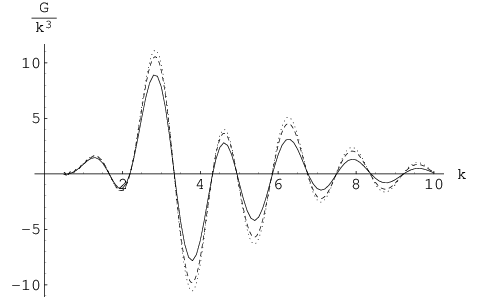
The resulting integral is now convergent for any we encounter in this work, and can be evaluated efficiently. We could repeat this process to further speed the convergence of the remaining integral, but in practice this is not necessary. We illustrate the effectiveness of this “boundary regulator” in Figure 1.
4 Horizon scale generation of non-Gaussianities
In this section, we explore models of inflation where the non-Gaussianities are generated when the modes cross the horizon. Typically these models require a violation of slow-roll at some fixed physical scale. All modes experience a temporary boost in their coupling strengths courtesy of this violation, but only modes exiting the horizon as the violation occurs receive a boost in their non-Gaussian signatures. Modes deep within the horizon are still rapidly oscillating, and the net contribution to their non-Gaussianities cancel. The violation of slow roll can have two origins. The first is a potential with a localized feature, as discussed in [38], and we now generalize this analysis. Secondly, if the duration of inflation is such that initial transients in the dynamics have not been erased before observable modes leave the horizon [49] we again find a significantly boosted 3-point function at these scales, even though the potential is smooth.
4.1 Features in the inflationary potential
Consider a small step in the inflaton potential [36]. In the limit that the step is a genuine discontinuity, the change in the potential energy across the step would be entirely converted into the inflaton’s kinetic energy, which is then damped away. For realistic models so across the step, and . Recall that we are working in the Hubble slow roll formalism – if we had defined this quantity can become large across the step. Further, is the rate of change of , so and can become large, provided they do so over a small enough range in . Features are thus associated with a characteristic physical scales and thus generate scale-dependent power spectra and higher correlation functions [38].
The 3-point correlation function is dominated by the term [38],
| (4.19) |
In [38], we introduced the to describe non-Gaussianities with both shape and scale dependence:
| (4.20) |
where is a constant, and for convenience we set it to be roughly equal to the magnitude of the power spectrum, . In the absence of the sharp feature, (4.20) reduces to the local form with in WMAP’s convention. We now construct an analytic approximation to this function.
To illustrate our approach, we consider two specific features, the step [36, 38]
| (4.21) |
and the bump
| (4.22) |
where , and again respectively determines the height, width and location of the feature. In the latter case, must be small enough to ensure that the field point does not get trapped in a local minimum. We present the numerical results for in Fig. 2 and the non-Gaussianity profile in Figure 3.

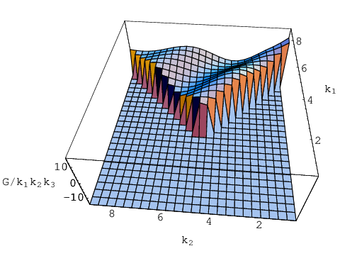
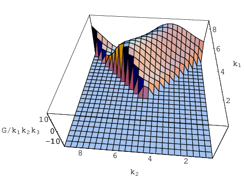
As we see from Fig. 2, is non-trivial over a small range of , but we do not have an analytic result for , and in [38] we performed these integrals numerically. Now consider a series of hat functions, , for , and otherwise. Outside the range of these hat functions, , so
| (4.23) |
Namely, the area under the hat functions or the numerical curve of should sum to approximately zero. We approximate by its unperturbed form
| (4.24) |
although the actual mode functions can deviate from this simple form by as much as a factor of two (in addition to phase shifts) for short periods of time [36]. Using these approximations,
| (4.25) | |||||
where
| (4.27) |
and denotes the imaginary part of the exponential integral function. For , ; for , .


For large , , Eq. () is dominated by the last term,
| (4.28) |
Numerically, the dominant scale-dependent oscillation comes from the term , where is the center of the hat function, and corresponds to the moment the inflaton crosses the feature and . We denote this scale . The amplitude is further modulated by . Typically , so this terms is less important unless the non-Gaussianities are found over a large -range. From (4.23), we see the amplitude of (4.28) is roughly ( is the duration of the feature in ). This amplitude is consistent with the order-of-magnitude estimate of Ref. [38].
Before we write down the ansatz, let us take a step back and consider several other limits not well described by Eq. (4.28). For small , , and the leading terms (the first two terms in ()) are proportional to . So the next order terms dominate,
| (4.29) |
The non-Gaussianities vanish as as these modes are outside the horizon as the inflaton encounters the feature.
In the squeezed triangle limit, and , the second term in () dominates instead of the third and we have a different behavior
| (4.30) |
Comparing (4.28) and (4.30), we see that the latter becomes more important if one of the momenta is smaller than . This is less important observationally than Eq. (4.28), as it requires measurements on two widely different scales. In addition, Eq. (4.28) is incomplete also because it does not vanish for large , and this is an artifact of the sharp edge of our hat functions. We expect (4.28) to decay away after a width where is the smoothing of the sharp edge of the hat function.
With these caveats in mind, we can now write down the ansatz following Eq. (4.28) by defining
| (4.31) |
where we match the phase to our numerical results. We could improve this approach by taking a sum of a series of hat functions, so the final form of the 3-point correlation function would then be a sum over oscillatory functions
| (4.32) |
where is the scale associated with the center of the -th hat function, or further polish this result using an Euler-Maclaurin expansion. However, our primary goal here was to produce an analytic expression that mirrored the qualitative form of the 3-point function generated by a step, and in this we have succeeded. This expression is scale-dependent and thus differs from “local” and “equilateral” forms. Finally, this ansatz is clearly factorizable and in future work we will use it – in combination with the algorithms of [34] – to probe the ability of specific CMB experiments to recover this type of signal from data.
For the step potential [38],
| (4.33) |
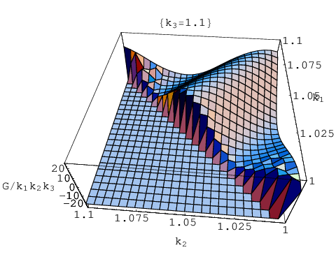
where and are the height and width of the step respectively. This feature is approximately localized, with a single scale . The derivation of the phase factor is not instructive and we obtained it by matching to our numerical results. Refs. [50, 51] use a step to explain the “glitch” seen in the temperature for , and find best fit parameters . Looking at Fig. 4 we find
| (4.34) |
The amplitude is within the order of magnitude that we expected from Eq. (4.33) and is indeed around the center of the feature in Fig. 2. These approximations are intended to capture the qualitative form of the 3-point function and do not have a high degree of numerical fidelity, but could certainly be further developed. Moreover, the detailed numerical match to the exact result could be improved substantially by adding heuristic parameters to the approximation, and then varying these to optimize the approximation.
4.2 Non-attractor initial conditions
Non-Gaussianities can also be enhanced if the inflaton trajectory is initially displaced from its attractor, slow-roll solution – for instance by giving it large kinetic energy (“fast-roll”) or perturbing the field point in a steep direction, orthogonal to the inflaton trajectory. Hubble friction will erase this transient, so this situation only arises when the overall duration of inflation is close to the minimal value. Again, modes that are crossing the horizon during this period have their non-Gaussianities boosted due to the enhanced coupling. In this case the relevant scales are the longest modes that contribute to the CMB.
This mechanism was used by Contaldi et. al. [49] to explain the possible low- suppression in CMB (see also [52, 53]).22 2 Ref. [54] extended this approach to other non-inflationary initial conditions, and the same conclusion applies to this model. Conversely, [55] looks at a perturbation in a two-field model, which is beyond the scope of the current analysis. The inflaton is started with a large velocity and the potential is negligible, so
| (4.35) |
One finds , and , where is determined by the initial velocity. During this fast-roll period,
| (4.36) |
In a qualitative estimate, Ref. [49] assumes that the slow-roll inflation period begins immediately after this kinetic-energy-dominated fast-roll (non-inflationary) period, and during slow-roll
| (4.37) |
Let us estimate the non-Gaussianity. For example, consider (A.69)
| (4.38) |
The fast-roll period is not inflationary, so modes are entering the horizon during this phase. As we will explain more quantitatively in Appendix B, we are interested in the modes that are slightly within the horizon as inflation begins. Modes that are near the horizon have smaller non-Gaussianities. Although the coupling is greatly enhanced comparing to in the slow-roll phase, the mode function is greatly suppressed. Looking at (4.38), we find the following factors of in the amplitude of the 3-point correlation
| (4.39) |
The first factor is the large coupling; the second is due to the asymptotic value , which is determined by the slow-roll inflation period; the third is from during the fast-roll period – note this is where the suppression comes from; the fourth is from the prefactor, , in the definition of . This gives
| (4.40) |
which is confirmed by a more detailed estimate in Appendix B.
We next look at the transition period from the end of the fast-roll to the slow-roll, where drops from to . This period is absent in the above analytical model of Ref. [49], but it also has important contribution to the non-Gaussianities. Once the kinetic and potential energies are roughly balanced, is approximately constant, and drops as and drops as . The grows from to at the beginning of this period, then drops to in the end. The most important contribution to the 3-point is the term, similarly to the sharp feature case, and possess the amplitude
| (4.41) |
The shape and running of this non-Gaussianity is also similar to those of the sharp feature, hence the ansatz (4.31) applies.
The sum of these two contributions implies that the 3-point is larger than the of standard slow-roll inflation. Our numerical simulation (not shown here) confirms this expectation. This is only comparable to the 3-point expected from simple non-linear gravitational effects of [1], and an order of magnitude smaller than the 3-point we found for a bump. Since the kinetic energy is simply redshifted away by the expansion of the universe, we cannot easily enhance this signal by tuning the potential. Further, this signal peaks at scales where cosmic variance will be largest, so we are not optimistic this signal will be observable, even under ideal conditions.
5 Sub-horizon generation of non-Gaussianities: Resonance model
We now turn our attention to the generation of significant non-Gaussianities while the modes are still well within the horizon. Again, we inspect the integral representation of the 3-point correlation function, Eq. (3.11). Modes that are well within the horizon oscillate rapidly. Since the interaction couplings are roughly constant for plain vanilla slow-roll model, these oscillations cancel. However, if the interaction couplings oscillate, they can interfere constructively with the rest of the integrand, yielding an enhanced 3-point signal. These contributions are generated while the modes are deep inside the horizon, and are thus physically distinct from the situation explored previously.
When all modes are inside the horizon, each of the 3-point integrals (3.11) consist of an oscillatory piece and a prefactor which is a function of the slow roll parameters. If the potential has a small oscillatory component, becomes
| (5.42) |
where , and . We assume that , and change slowly over a single Hubble time, and treat them as constants in what follows. As the physical wavelength increases, the mode will briefly resonate with the coupling term when its frequency is roughly . During this resonance phase, the term in the integrand of (3.11) can interfere constructively and generate a large 3-point function. Conversely, destructive interference will generate no extra contribution to the 3-point function. See Fig. 5 for an illustration of the resonance effect.

This resonance requires
| (5.43) |
in order to ensure that the relevant modes are sub-Planckian during the resonance epoch. In practice, this is not a strong constraint, but the resonance introduces a new length-scale into our analysis of cosmological perturbations.33 3 In models with a non-trivial UV cutoff below the Planck scale, this scale would replace in (5.43). In this case, we expect non-Gaussianities to be present at all scales, since the ripple is laid down across the entire potential, in contrast to the “features” considered above. Moreover, the modulation of the potential must be small enough to ensure that the inflaton does not get trapped – and if we make it small enough, we can also ensure that the 2-point function is not significantly modified even if the non-Gaussianities are large, as discussed in Appendix C.
To study this mechanism explicitly, consider a standard slow-roll model with a very small oscillatory component
| (5.44) |
Since is slowly rolling, the resonance effect occurs when the physical frequency reaches
| (5.45) |
Therefore to satisfy the resonance condition (5.43), we need and , while we take , in accordance with slow roll. In Appendix C we show that we need , so the perturbation to is small.
Before we proceed, we emphasize that (5.44) is simply a toy model, with no direct physical motivation. However, in brane inflation, it has been argued that the duality cascade within a throat will leave tiny sharp features in the inflaton potential or the background warp factor [56]. Such features typically come in a series and can have cosmologically observable effects as the inflaton branes roll across them [39]. If these features are large and well-separated, they would yield of sequence of isolated sharp features. However, in the opposite limit, one would have a situation closer to the modulated potential above.
We now estimate the resulting 3-point function. For definiteness, we use the following parameters in our numerical examples
| (5.46) |
The non-Gaussianity oscillates with because has a continually changing phase. The time it takes the inflaton to cross one “ripple” is , during which . So the oscillation period of this non-Gaussianity in -space is
| (5.47) |
Using the parameters in (5.46), this gives . This agrees with the numerical results shown in Fig. 6. We emphasize that the property is model-independent, since, ignoring the slow-variation of background evolution, the analysis for and is scale-independent. Another universal property is , via (5.43).
We now estimate the amplitude of these non-Gaussianities. The frequency of each mode is continuously decreasing due to the expansion of the universe. Once it differs from the resonant frequency by , the integration in the 3pt starts to cancel out if it is performed over . Meanwhile, it takes to stretch a mode sufficiently in order to induce a frequency change to . Equating and gives the time period over which resonance occurs for this particular mode,
| (5.48) |
In (5.44), this corresponds to the number of oscillation cycles
| (5.49) |
we need to integrate over, where is the oscillation period of the background. For (5.46) we need about cycles, which is confirmed numerically in Fig. 5.
The dominant source of 3-point terms – as for the “feature” models – is the interaction term Eq. (4.19). Because the mode is well within the horizon , in (4.25) the last term dominates. Denoting the oscillatory behavior of the slow-roll parameter as
| (5.50) |
where the subscript “A” denotes the oscillation amplitude. Integrating over one period
| (5.51) |
gives the amplitude , where is evaluated around the resonant point. Combining this with Eq. (5.49), from (4.25) we get the estimate of the amplitude
| (5.52) |
To evaluate (5.52), we need . For (5.44) the amplitude of the dominant oscillating term in is (see Appendix C)
| (5.53) |
Note one might naively expect that , i.e. that it scales as . However this over predicts the amplitude by a factor of : although , since via the scalar field equation of motion (2.3) and hence . It follows that . The crucial point is that one can always use Eq. (2.3) to eliminate one derivative of in the derivation of ; in other words one cannot simply neglect the term in the equation of motion. Numerical computations of show that this estimate Eq. (5.53) is accurate in both amplitude and scaling.
Combining (5.52) and (5.53), we get the amplitude
| (5.54) |
where we have restored into the final answer. For (5.46), , which differs from matches to our exact numerical results shown in Fig. 6 by . The numerical results also exhibit the scaling, as can been seen in Fig. 7.
The ansatz for the non-Gaussianity is therefore
| (5.55) |
where
| (5.56) |
The comes from the fact [in Eq. (5.47)] that the oscillation period is proportional to and the background dependence of is approximately scale-invariant. The value of is determined by the oscillation frequency in the -space. We also point out that the power spectrum has the same oscillatory frequency in -space, due to the same reason that we stated before (5.47). See Fig. 8 in Appendix C for details. We compare this ansatz with the numerical result in Fig. 6. This ansatz is factorizable at least by Taylor-expanding in a range smaller than . Note unlike the ansatz for the feature (4.31) where the non-Gaussianities are peaked around some fixed scale , the amplitude does not decay and is present at all scales. In addition, so it oscillates faster. As we noted above, the specific potential we consider is a toy model, but this analysis could be extended to more complicated modulations, or models where the modulation applied only over a finite range of field values.


6 Discussion and Conclusion
We studied two distinctly mechanisms for generating large non-Gaussianities within single field inflation. We derive the approximate 3-point correlation functions using semi-analytic methods, which are in the computationally useful factorizable form. In the first mechanism, non-Gaussianity is generated at horizon crossing by either a feature in the potential, or an initial transient in the inflationary dynamics. In the second case, oscillating slow roll parameters induce a resonance which leads to the generation of a non-Gaussian signal well before horizon crossing. In both cases, the 3-point function depends strongly on the individual wavelengths of the modes in the “triangle”. With a single, sharp feature or non-standard initial conditions, the 3-point is only enhanced in modes which are crossing the horizon as the inflaton traverses the “feature”. In a resonance model such as (5.44), the physical non-Gaussianity is present at all scales.
In the resonance case, we showed that the 3-point function is periodic with a period proportional to, and smaller than, . This non-Gaussianity will peak starting from a fixed scale when projected onto the CMB sky. Assume for simplicity that where is the CMB multipole, and denote as the oscillation period. At larger scales where the oscillation spanning , this non-Gaussianity presumably cannot be resolved experimentally. For the numerical example considered here, it would become visible at where starts to exceed , inducing an effective scale-dependence in this signal.
With a feature in the potential, the resulting transient violation of slow-roll generically leads to an oscillatory and scale-dependent 3-point function. We wrote down a heuristic and factorizable scale-dependent expression for this signal and showed that it captured the qualitative properties seen in the exact numerical evaluations of the corresponding integrals. The 3-point correlation decays as we move away from , where corresponds to the scale leaving the horizon as the inflaton traverses the feature. We also show that while non-standard initial conditions such as the fast-roll model of [49] can generate large non-Gaussianities relative to our usual expectations for single field inflation, the amplification is not expected to lift them above the “noise” of non-linearities produced by post-inflationary gravitational evolution alone.
In addition, we have presented detailed description of a general numerical method for computing the 3-point correlation functions of primordial perturbations from canonical single scalar field inflationary models with arbitrary potentials. We show that while the integrals themselves are formally convergent, they need to be regularized as the integrands are oscillatory, and show how this can be accomplished analytically, rendering the numerical integrals rapidly convergent.
There is much further work to be done. Our immediate goal [57] is to use our heuristic ansatzen to construct an optimal estimator with which to search for scale-dependent non-Gaussianities in the cosmic microwave background, and estimate the likely bounds that future missions can put on this signal. On the theoretical front, we plan to investigate the details of non-Gaussianities generated by multi-field models [5, 7] within the horizon, and with non-standard kinetic terms. Moreover, while the analytic approximations we present here capture the qualitative form of the 3-point function, they are not intended to provide a precise quantitative match to the numerically computed values, but these approximations can certainly be improved.
Acknowledgments
We thank Eiichiro Komatsu, Henry Tye, Jiajun Xu, Hiranya Peiris, Kendrick Smith and Sarah Shandera for valuable discussions. XC and EAL would like to thank the Kavli Institute for Theoretical Physics in China and the organizers of the “String Theory and Cosmology” program, where part of this work is done, for their warm hospitality. XC is supported by the US Department of Energy under cooperative research agreement DEFG02-05ER41360. RE is supported in part by the United States Department of Energy, grant DE-FG02-92ER-40704.
Appendix A 3-point correlation functions
In minimally coupled single field inflation, the cubic interaction Hamiltonian for the scalar perturbation is [3, 46, 15]
| (A.57) | |||||
where
| (A.58) |
Here is the inverse Laplacian. This cubic Hamiltonian is exact for arbitrary and .
The 3-point correlation function at some time after horizon exit is
| (A.59) |
together with a term coming from the field redefinition
| (A.60) | |||||
where denotes the Fourier transform of .
We evaluate it using the decomposition
| (A.61) | |||
| (A.62) |
where is the solution of the linear equation of motion of the quadratic action,
| (A.63) |
Our choice of vacuum implies that the initial condition for the mode function is given by the Bunch-Davies vacuum
| (A.64) |
where we have neglected an irrelevant phase.
We get seven contributions. The terms proportional to arise from the term
| (A.65) |
the term
| (A.66) |
and the term
| (A.67) |
The term proportional to is
| (A.68) |
The terms proportional to include that from term
| (A.69) |
and that from term
| (A.70) |
The field redefinition (A.60) contributes
| (A.71) |
In these equations, the “two perm” stands for two other terms that are symmetric under permutations of the indices 1, 2 and 3.
In Ref. [3, 46, 15] where sharp features and non-attractor initial condition are absent, terms (A.65), (A.66), (A.67) and (A.71) give the leading contributions to non-Gaussianities. In Ref. [38] where features are present on an otherwise flat potential, term (A.68) is the leading term. For the non-attractor initial condition that we consider in Sec. 4.2, the terms (A.69) and (A.70) can also give important contributions in addition to other terms, because and can be large initially.
Appendix B Non-Gaussianities from initial conditions
In this appendix, we give some details on the estimate of non-Gaussianity from the fast-roll period discussed in Sec. 4.2. In terms of the conformal time , the scale factor of the fast-roll period becomes
| (B.72) |
Here the fast-roll starts at and end at . is the conformal Hubble parameter evaluated at the beginning the slow-roll inflation period (i.e. the end of the fast-roll period) . is the corresponding Hubble parameter in terms of , . This fast-roll period is immediately connected to the inflation period in which the scale factor grows as
| (B.73) |
We first look at the power spectrum discussed in [49]. Using (B.72), one gets
| (B.74) | |||
| (B.75) |
From the definition , we get
| (B.76) |
Picking a special initial condition for , the equation of motion can be solved as
| (B.77) |
where is the second Hankel function with index . Requiring this solution and its first derivative to continuously match to the slow-roll results
| (B.78) |
at determines the coefficients and
| (B.79) |
The power spectrum is
| (B.80) |
At large scale for ,
| (B.81) |
Hence we see that as resulting a suppression for the large scales. For , it relaxes to the usual attractor value .
Now we estimate the order of magnitude of the contribution to 3-point function by this fast-roll period. As an example, we look at the terms (A.69) and (A.70). The terms are expected to be of a similar size. We look at the modes so the asymptotic value of at the end of inflation is approximately that of the slow-roll inflation,
| (B.82) |
as we see from the discussions in the last paragraph.
The net contribution of (A.69) and (A.70) to the 3pt is
| (B.83) |
where
| (B.84) |
We have integrated from the start of the fast-roll period to the beginning of the slow-roll period . We have written the lower limit of the integration in terms of the Hubble parameter at the beginning of the fast-roll, .
Comparing to the WMAP’s ansatz in the limit
| (B.85) |
we get a scale dependent amplitude for this fast-roll period
| (B.86) |
The integrand in (B.84) starts oscillating for large . So for very large , , this integration approaches zero. Therefore, we look at the modes . For example, for , , , , we have and . This is consistent with the rough argument given in (4.39).
Appendix C Slow-roll parameters in the resonance model
In this appendix, we work out some details on the behavior of the slow-roll parameters in the resonant model. Using (5.44) as the explicit example, we decompose (and similarly for other variables)
| (C.87) |
where the is the unperturbed background evolution, and is the oscillation caused by the small high frequency ripples imposed on the potential. Since the oscillation frequency , the equation of motion for the oscillatory part is
| (C.88) |
where the term is much smaller than and neglected. The dominant contribution to comes from
| (C.89) |
Using the background evolution
| (C.90) |
we can solve (C.88) and get
| (C.91) |
With this result, one can check that (C.89) is indeed the leading oscillatory term in (5.44).
We next calculate the oscillatory part of and . Differentiating
| (C.92) |
we get
| (C.93) |
So, we have
| (C.94) |
From (C.94), we get
| (C.95) |
Note that if we try to get from (C.92), the leading terms will cancel and the subleading terms are not reliable in our approximation.

Now we calculate the oscillatory part of the slow-roll parameters. It is easy to see from the above results that the leading correction term for comes from that for , so
| (C.96) | |||||
The leading correction term for comes from that for ,
| (C.97) | |||||
Taking the time derivative of the above equation (C.97) we get
| (C.98) |
which we can also derive directly by plugging in the potential Eq. (5.44) into the definiton for , Eq. (2.6), and keeping the leading oscillatory term.
The most important term in the linear equation of motion (A.63) is
| (C.99) |
The most significant oscillating component comes from the last term
| (C.100) |
This term causes a dramatic oscillation of the freeze-out scale of the perturbation, which we define to be . For example, in terms of the numerical number (5.46), the amplitude of (C.100) is , of the same order of the non-oscillating component . The horizon size that we used in the main text refers to the averaged non-oscillating component. This oscillation affects the power spectrum, which we present numerically in Fig. 8. The oscillation in the power spectrum is tiny, but is potentially observable if the fidelity of our CMB data is very high. The structure of these oscillations is reminiscent of those of the “trans-Planckian” models of inflation, but with the distinctive scale-dependent oscillation frequency which has the same properties as we discussed at the end of Sec. 5 for the non-Gaussianity. For relevant details on constraining such oscillatory power spectrum on the CMB sky, see Ref. [58, 59].
References
- [1] T. Pyne and S. M. Carroll, Phys. Rev. D 53, 2920 (1996) [arXiv:astro-ph/9510041].
- [2] V. Acquaviva, N. Bartolo, S. Matarrese and A. Riotto, Nucl. Phys. B 667, 119 (2003) [arXiv:astro-ph/0209156].
- [3] J. M. Maldacena, JHEP 0305, 013 (2003) [arXiv:astro-ph/0210603].
- [4] G. I. Rigopoulos, E. P. S. Shellard and B. J. W. van Tent, arXiv:astro-ph/0511041.
- [5] D. Seery and J. E. Lidsey, JCAP 0509, 011 (2005) [arXiv:astro-ph/0506056].
- [6] F. Vernizzi and D. Wands, JCAP 0605, 019 (2006) [arXiv:astro-ph/0603799].
- [7] T. Battefeld and R. Easther, JCAP 0703, 020 (2007) [arXiv:astro-ph/0610296].
- [8] S. Yokoyama, T. Suyama and T. Tanaka, arXiv:0705.3178 [astro-ph].
- [9] E. Silverstein and D. Tong, Phys. Rev. D 70, 103505 (2004) [arXiv:hep-th/0310221].
- [10] M. Alishahiha, E. Silverstein and D. Tong, Phys. Rev. D 70, 123505 (2004) [arXiv:hep-th/0404084].
- [11] X. Chen, Phys. Rev. D 71, 063506 (2005) [arXiv:hep-th/0408084].
- [12] X. Chen, JHEP 0508, 045 (2005) [arXiv:hep-th/0501184].
- [13] C. Armendariz-Picon, T. Damour and V. F. Mukhanov, Phys. Lett. B 458, 209 (1999) [arXiv:hep-th/9904075].
- [14] J. Garriga and V. F. Mukhanov, Phys. Lett. B 458, 219 (1999) [arXiv:hep-th/9904176].
- [15] X. Chen, M. x. Huang, S. Kachru and G. Shiu, JCAP 0701, 002 (2007) [arXiv:hep-th/0605045].
- [16] M. Li, T. Wang and Y. Wang, arXiv:0801.0040 [astro-ph].
- [17] R. Bean, D. J. H. Chung and G. Geshnizjani, arXiv:0801.0742 [astro-ph].
- [18] D. H. Lyth, C. Ungarelli and D. Wands, Phys. Rev. D 67, 023503 (2003) [arXiv:astro-ph/0208055].
- [19] B. Chen, Y. Wang and W. Xue, arXiv:0712.2345 [hep-th].
- [20] S. Gupta, A. Berera, A. F. Heavens and S. Matarrese, Phys. Rev. D 66, 043510 (2002) [arXiv:astro-ph/0205152].
- [21] I. G. Moss and C. Xiong, JCAP 0704, 007 (2007) [arXiv:astro-ph/0701302].
- [22] N. Barnaby and J. M. Cline, arXiv:0704.3426 [hep-th].
- [23] N. Arkani-Hamed, P. Creminelli, S. Mukohyama and M. Zaldarriaga, JCAP 0404, 001 (2004) [arXiv:hep-th/0312100].
- [24] C. Cheung, P. Creminelli, A. L. Fitzpatrick, J. Kaplan and L. Senatore, arXiv:0709.0293 [hep-th].
- [25] E. Komatsu and D. N. Spergel, Phys. Rev. D 63, 063002 (2001) [arXiv:astro-ph/0005036].
- [26] E. Komatsu, D. N. Spergel and B. D. Wandelt, Astrophys. J. 634, 14 (2005) [arXiv:astro-ph/0305189].
- [27] D. Babich, P. Creminelli and M. Zaldarriaga, JCAP 0408, 009 (2004) [arXiv:astro-ph/0405356].
- [28] D. N. Spergel et al. [WMAP Collaboration], arXiv:astro-ph/0603449.
- [29] P. Creminelli, L. Senatore and M. Zaldarriaga, JCAP 0703, 019 (2007) [arXiv:astro-ph/0606001].
- [30] P. Creminelli, L. Senatore, M. Zaldarriaga and M. Tegmark, JCAP 0703, 005 (2007) [arXiv:astro-ph/0610600].
- [31] A. P. S. Yadav, E. Komatsu, B. D. Wandelt, M. Liguori, F. K. Hansen and S. Matarrese, arXiv:0711.4933 [astro-ph].
- [32] A. P. S. Yadav and B. D. Wandelt, arXiv:0712.1148 [astro-ph].
- [33] D. S. Salopek and J. R. Bond, Phys. Rev. D 42, 3936 (1990).
- [34] K. M. Smith and M. Zaldarriaga, arXiv:astro-ph/0612571.
- [35] J. R. Fergusson and E. P. S. Shellard, arXiv:astro-ph/0612713.
- [36] J. A. Adams, B. Cresswell and R. Easther, Phys. Rev. D 64, 123514 (2001) [arXiv:astro-ph/0102236].
- [37] E. Komatsu et al. [WMAP Collaboration], Astrophys. J. Suppl. 148, 119 (2003) [arXiv:astro-ph/0302223].
- [38] X. Chen, R. Easther and E. A. Lim, JCAP 0706, 023 (2007) [arXiv:astro-ph/0611645].
- [39] R. Bean, X. Chen, G. Hailu, S. H. Tye and J. Xu, arXiv:0802.0491 [hep-th].
- [40] D. S. Salopek and J. R. Bond, Phys. Rev. D 43 (1991) 1005.
- [41] M. Sasaki and E. D. Stewart, Prog. Theor. Phys. 95, 71 (1996) [arXiv:astro-ph/9507001].
- [42] C. T. Byrnes, K. Koyama, M. Sasaki and D. Wands, arXiv:0705.4096 [hep-th].
- [43] D. H. Lyth and Y. Rodriguez, Phys. Rev. Lett. 95, 121302 (2005) [arXiv:astro-ph/0504045].
- [44] S. Weinberg, Phys. Rev. D 72, 043514 (2005) [arXiv:hep-th/0506236].
- [45] J. M. Bardeen, Phys. Rev. D 22 (1980) 1882.
- [46] D. Seery and J. E. Lidsey, JCAP 0506, 003 (2005) [arXiv:astro-ph/0503692].
- [47] C. M. Bender and S. A.Orszag, Advanced Mathematical Methods for Scientists and Engineers, Springer-Verlag (1999).
- [48] J. Martin and D. J. Schwarz, Phys. Rev. D 67, 083512 (2003) [arXiv:astro-ph/0210090].
- [49] C. R. Contaldi, M. Peloso, L. Kofman and A. Linde, JCAP 0307, 002 (2003) [arXiv:astro-ph/0303636].
- [50] H. V. Peiris et al. [WMAP Collaboration], Astrophys. J. Suppl. 148, 213 (2003) [arXiv:astro-ph/0302225].
- [51] L. Covi, J. Hamann, A. Melchiorri, A. Slosar and I. Sorbera, Phys. Rev. D 74, 083509 (2006) [arXiv:astro-ph/0606452].
- [52] D. Boyanovsky, H. J. de Vega and N. G. Sanchez, Phys. Rev. D 74, 123006 (2006) [arXiv:astro-ph/0607508].
- [53] D. Boyanovsky, H. J. de Vega and N. G. Sanchez, Phys. Rev. D 74, 123007 (2006) [arXiv:astro-ph/0607487].
- [54] B. A. Powell and W. H. Kinney, Phys. Rev. D 76, 063512 (2007) [arXiv:astro-ph/0612006].
- [55] C. P. Burgess, J. M. Cline, F. Lemieux and R. Holman, JHEP 0302, 048 (2003) [arXiv:hep-th/0210233].
- [56] G. Hailu and S. H. Tye, JHEP 0708, 009 (2007) [arXiv:hep-th/0611353].
- [57] X. Chen, R. Easther, E. Komatsu, H. Peiris, E. A. Lim and K. Smith, In preparation
- [58] T. Okamoto and E. A. Lim, Phys. Rev. D 69, 083519 (2004) [arXiv:astro-ph/0312284].
- [59] R. Easther, W. H. Kinney and H. Peiris, JCAP 0508, 001 (2005) [arXiv:astro-ph/0505426].