From short to fat tails in financial markets: A unified description
Abstract
In complex systems such as turbulent flows and financial markets, the dynamics in long and short time-lags, signaled by Gaussian and fat-tailed statistics, respectively, calls for a unified description. To address this issue we analyze a real dataset, namely, price fluctuations, in a wide range of temporal scales to embrace both regimes. By means of Kramers-Moyal (KM) coefficients evaluated from empirical time series, we obtain the evolution equation for the probability density function (PDF) of price returns. We also present consistent asymptotic solutions for the timescale dependent equation that emerges from the empirical analysis. From these solutions, new relationships connecting PDF characteristics, such as tail exponents, to parameters of KM coefficients arise. The results reveal a dynamical path that leads from Gaussian to fat-tailed statistics, furnishing insights on other complex systems where akin crossover is observed.
pacs
05.10.Gg, 05.40.-a, 89.65.GhOne of the main problems in statistical physics consists in the study of macroscopic changes of systems in which fluctuations play a central role, e.g., diffusion and noise-induced transitions. The Fokker-Planck equation (FPE) [1] provides a powerful tool for dealing with such problems and has been used in many different fields in natural sciences, including solid-state and plasma physics, quantum optics, chemical and nuclear reaction kinetics, molecular biology and population dynamics. Financial data have also been described as stochastic processes governed by Langevin or FPEs. These efforts are of utter relevance due to the strongly complex fluctuating dynamics of financial time series, which poses new challenges to model the dynamical laws responsible for the observed statistical properties. In that direction, for example, the anomalous diffusive properties and second-order correlations of price fluctuations (e.g., see [2]), have been addressed through multivariate [3] and non-linear [4] models. However, these attempts are usually built phenomenologically and, as far as they are manifold, entail drawbacks for unmasking the processes that rule the underlying dynamics.
A typical feature of complex systems is the existence of non-trivial structures on different timescales. In particular, the dynamics of price fluctuations in long and short timescales, signaled by Gaussian and fat-tailed probability density functions (PDFs), respectively, has been usually treated in the literature separately, and a unified description in the full range of timescales is still lacking.
Our present goal is two-fold. The first one is to grasp, through a non-parametric method, the underlying stochastic dynamics of price fluctuations in order to unveil the driving mechanisms within a unified framework. The second one is to determine analytically, from the stochastic equations that emerge from the first step, the family of PDFs that encompasses the observed timescale dependent ones. To these ends, we obtain the evolution equation for the PDF of price returns through the estimation of Kramers-Moyal (KM) expansion coefficients. We follow the work by Friedrich and collaborators [5, 6], which exploits a correspondence between financial market dynamics and hydrodynamic turbulence [7] assuming the existence of a flux of information towards finer scales. This approach has been applied before for developed markets, although for limited time windows [5, 8, 9, 10]. Here, as a relevant example, we scrutinize the daily and intraday time series of Ibovespa, the financial index of the Brazilian stock market, which is not fully understood, despite typifying major emergent markets. We address a large hierarchy of time-lags, ranging from months to minutes. From the measured KM coefficients, we are able to reproduce the full evolution of empirical histograms of price returns, embracing the crossover from Gaussian to strongly fat-tailed PDFs when going from large to short timescales. We also present consistent solutions of the resulting FPE. They belong to the class of generalized Student-t distributions (also known in recent literature as -Gaussians [11]) that comprises the non-stationary invariant PDFs observed in both asymptotic limits.
We investigate the timescale evolution of the PDF of logarithmic price increments (returns) . We consider, as a general evolution equation for those PDFs, the KM expansion of a master equation, valid for Markov processes [1]:
| (1) |
where the coefficients are defined as
| (2) |
with , being the moments of the conditional PDFs, i.e., . Following the insight provided by cascade models in turbulence, we consider a logarithmic time scale defined as , where is a reference time-lag.
For the analysis of Ibovespa, we select three datasets: 3960 deflated daily closing prices, in the term 02Jan.1991-28Dec.2006, 37984 15-minute cotes in 21Jan.1998-31Mar.2003 and 794310 30-second cotes in 01Nov.2002-19Jul.2006. The timescale () is set as 32 (trading) days. In what follows, the measured returns are given in units of the standard deviation of the respective data sample at 32-day time-lag.
Markovianity was investigated by evaluating the Chapman-Kolmogorov equation [1]. We found that it holds, thus validating our approach. The KM coefficients were estimated directly from data series by means of their statistical definition, given by Eq. (2). Conditional PDFs , with , were obtained from the data sets by building the histograms for the joint PDFs , computed over pairs of returns , incident at the same initial time. The first coefficients were computed for and . For each couple of values (), we found that and , as a function of , follow, in very good approximation, linear and quadratic laws, respectively, as illustrated in Fig. 1. Namely,
| (3) | |||||

Similar behaviors for and have been observed for linear and logarithmic increments of indexes and exchange rates involving US, Germany and Japan markets[5, 8, 10]. By fitting the linear and quadratic ansatz to the data, we obtained the parameters for each (). For fixed , the limit in Eq. (2) was achieved by extrapolation of the parameters as a function of . For the fourth order KM coefficients , as a function of , fourth order polynomial fits were performed, the limit being consistent with vanishingly small . Therefore, according to Pawula theorem [1] the KM expansion (1) can be truncated after the second order, thus reducing to the form of a FPE. The limiting values determine the -dependence of drift, , and diffusion, , coefficients. The -dependence of the limiting parameters is presented in Figs. 2-3.
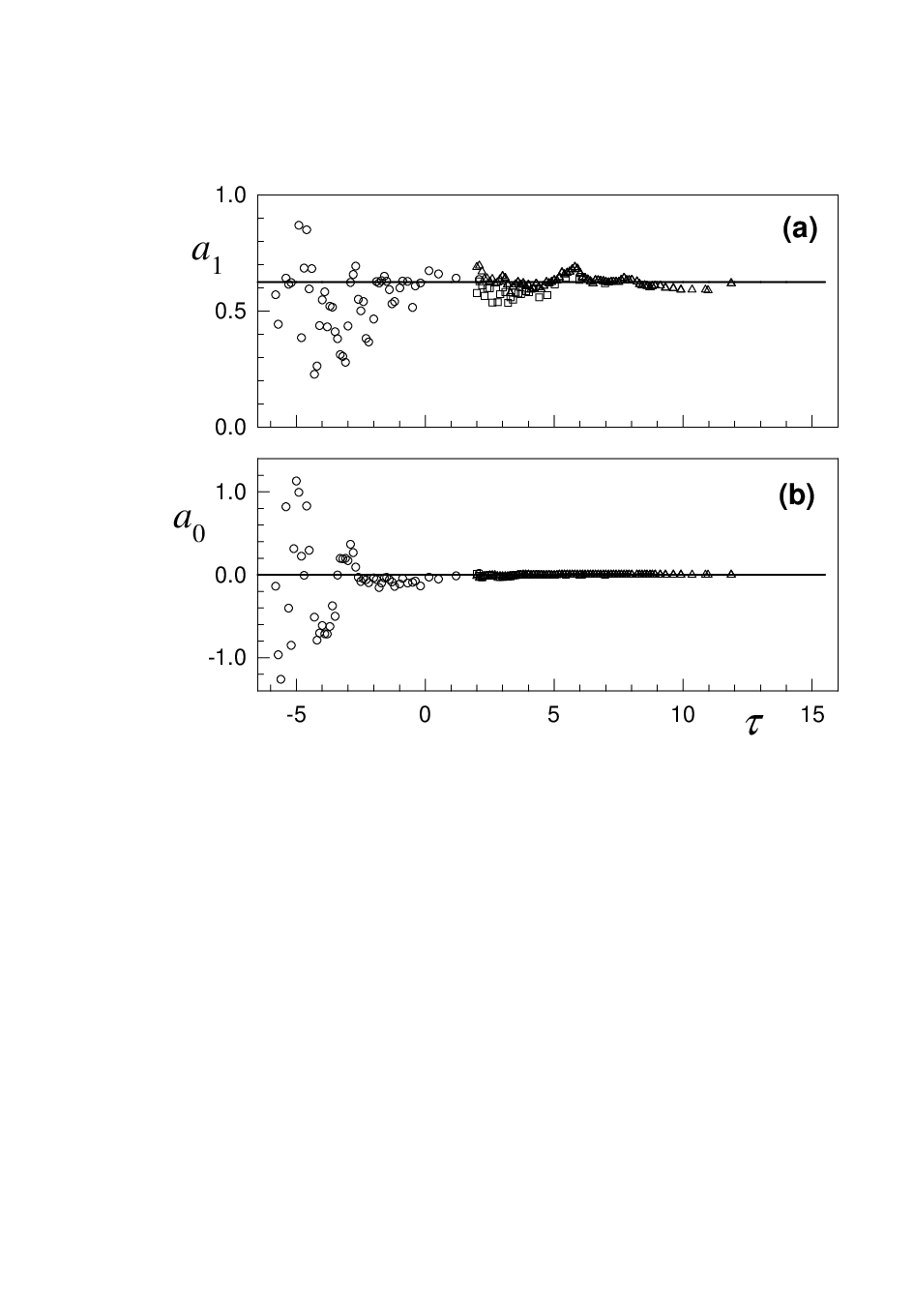


Parameters and describe the deviation of the PDFs from symmetry around zero. Indeed, this feature is observed for larger scales, where both parameters present non-null values, although with large fluctuations. In contrast, for intraday scales, and are negligible. Drift parameter remains approximately constant along daily and intraday time-scales. Diffusion parameter increases with from near zero up to a limiting value, signaling a crossover in the underlying dynamics at the monthly scale. Meanwhile, diffusion parameter presents a sustained exponential decay as increases. Similar behavior of was also reported for exchange rates [5], although for a shorter range of timescales. Despite the exponential-like decay of , it can not be neglected at large : representing the additive noise component, it provides stability to the stochastic process for small . In fact, the variance also follows an exponential-like decay , as shown in Fig. 3(c), thus setting the reference level for . Two limiting regimes associated with slightly different slopes are observed for both quantities (see Fig. 3(c)), suggesting that is related to . In the limit of small both quantities are characterized by , corresponding to normal diffusion, while in the limit of large , 1, showing the onset of superdiffusion in the high-frequency regime. For , data restrictions for obtaining small results prevent the estimation of the parameters.
The resulting FPE explicitly reads:
| (4) |
where the -dependence of the parameters was smoothed according to the ansatz plotted in Figs. 2-3. Eq. (4) was numerically integrated by means of a FTCS scheme [12]. A Gaussian fit to the empirical histogram at =128 days (), was used as initial condition. The evolution was carried out down to the scale of 30 seconds, the highest time resolution of our data. For 11, further evolution of the FPE, was performed by extrapolation of the -dependence of the coefficients. In Fig. 4, we show the PDFs of returns (rescaled by ) generated by the FPE, together with the empirical ones. Their agreement is remarkably good, in the full range of data, strongly supporting our estimation of KM coefficients.
Within Langevin dynamics, and are related to the deterministic and random forces, respectively [1]. Despite the wide range of analyzed time-lags, the intensity of the harmonic restoring force, given by , remains almost constant for . This means that the relaxation mechanisms that are governed, among other factors, by constraints, flux of information, stock liquidity, and risk aversion, act similarly at diverse temporal scales.
The evolution of the diffusion coefficient presents more distinctive features. For most timescales, is dominated by the state-independent and quadratic components, associated to additive and multiplicative noises, respectively. Due to the cumulative character of the fluctuations, the additive component increases with . Meanwhile, the change of to a higher plateau for small indicates large multiplicative effects in that region, that fade away in the opposite limit of large time-lags, as expected. This means that the endogenous behavior of the market, which spontaneously creates the amplification response mechanism to price fluctuations, presents different typical levels for micro and macro timescales.
The presence of multiplicative noise is known to be an ubiquitous mechanism to generate fat-tailed PDFs as steady-state solutions [13, 14]. It was found out that for a large set of control parameters, power-law tails prevail, with exponent depending on the ratio while being independent. Furthermore, Langevin dynamics mapped onto stochastic multiplicative processes with reinjection gives rise to power-law PDFs [15], from which the expression = was derived [16]. From these previous results, the observed plateaux of and suggest a -invariant tail of the PDF. In fact, the FPE (4) admits invariant solutions as discussed below.
Assuming an exponential law for , steady values of and , and neglecting , the solution of FPE (4) is
| (5) | |||||
| (6) |
where does not depend on time. Notice that Eq. (6) differs from the expression reported in [16]. The solution (5) is a -Gaussian (with ) [11]. In the particular case , the solutions become of the Gaussian form.
The rescaled variance is
| (7) |
In the limit of large time-lags, the diffusion coefficient is dominated by the state independent term that obeys . Substitution of the numerical values of and , into Eq. (7) yields, in very good approximation, (normal diffusion in the linear time scale) in agreement with numerical results (see Fig. 3(c)). As a consequence, in that limit, the evolution equation recovers Gaussianity, ruled by a balance between the deterministic harmonic force and the time dependent additive noise. In the opposite limit of large , attains a non-null steady value, while with . Also in this case, Eq. (7) predicts an asymptotic behavior of in agreement with empirical values, as depicted in Fig. 3(c).
As the evolution of the parameters other than is slow, especially for , we also checked if the PDFs could be effectively described by the ansatz (5) in an extended temporal regime. The outcomes of the fits match well the respective empirical PDFs, for almost any . For , the significantly non-null value of , imposes a correction to the -Gaussian form, yielding asymmetry. The values of resulting from (least squares) -Gaussian fits and are displayed in Fig. 5, together with the asymptotic value obtained from Eq. (6). For small , the increasing value of the effective points the onset of the Gaussian regime. For large , the empirical tail exponents tend to a steady value in good accord with the theoretical ones.

Power-law tails are often quoted in the literature for financial assets in high-frequency regimes [4, 17]. Ansatz of the -Gaussian form have been proposed before for high-frequency [4, 18] and for daily [9] logarithmic returns from a phenomenological approach. Meanwhile, in our case, they arise naturally from the evolution equation obtained empirically from the evaluation of KM coefficients throughout time-lags.
Let us recall that the results for (4 min), in Fig. 4, were obtained by extrapolation of the -dependence of the coefficients. However, a good foresight of the empirical histograms arises from FPE evolution up to =14.75 (=1 min). On one hand, this ensures the reliability of the estimated parameters; on the other, it accounts for the predictability of intraday statistics, due to the well known existence of memory effects in the high-frequency regime of price returns. It is worth to mention that the observed deviation of the empirical histogram for the smallest analyzed time-lag (30 seconds) expresses the beginning of a non-Markovian regime [19].
In sum, we have disclosed the evolutionary pattern of the empirical PDFs of price returns, from Gaussian to long-tailed regimes. Beyond the system under study, the scope of our results may be appropriate for a larger financial scenario. Moreover our findings are not restricted to the complexity of financial data, but may provide insights for systems on general physical contexts, such as in turbulent flows [20], where similar Gaussian to -Gaussian crossovers have been observed.
Acknowledgements.
We acknowledge Brazilian agency CNPq for partial financial support and BOVESPA for providing the data.References
- [1] Risken H., The Fokker-Planck Equation: Methods of Solution and Applications (Springer-Verlag, Berlin) 1984.
- [2] Mantegna R., Stanley H.E., An Introduction to Econophysics (Cambridge University Press, Cambridge) 2000.
- [3] Dragulescu A.A., Yakovenko V.M., Quantitative Finance, 2 (2002) 443.
- [4] Borland L., Phys. Rev. Lett., 89 (2002) 098701.
- [5] Friedrich R., Peinke J., Renner C., Phys. Rev. Lett., 84 (2000) 5224.
- [6] Lück St., Peinke J., Friedrich R., Phys. Rev. Lett., 83 (1999) 5495; Friedrich R., Peinke J., ibid., 78 (1997) 863.
- [7] Ghashghaie S., Breymann W., Peinke J., Talkner P., Dodge Y., Nature, 381 (1996) 767.
- [8] Ivanova K., Ausloos M., Takayasu H., cond-mat/0301268 preprint, 2003.
- [9] Ausloos M., Ivanova K., Phys. Rev. E, 68 (2003) 046122.
- [10] Karth M., Peinke J., in Complexity V. 8 (John Wiley & Sons Inc., New York) 2002.
- [11] Tsallis C., in Non-Extensive Entropy-Interdisciplinary Applications, edited by Gell-Mann M. and Tsallis C. (Oxford University Press, Oxford) 2004.
- [12] Press W.H., Flannery B.P., Teukolsky S.A., Vetterling W.T., Numeric Recipes. The Art of Scientific Computing (Cambridge University Press, Cambridge) 1986.
- [13] Schenzle A., Brand H., Phys. Rev. A, 20 (1979) 1628.
- [14] Anteneodo C., Tsallis C., J. Math. Phys., 44 (2003) 5194; Anteneodo C., Riera R., Phys. Rev. E, 72 (2005) 026106.
- [15] Takayasu H., Sato A.H., Takayasu M., Phys. Rev. Lett., 79 (1997) 966; Sornette D., Phys. Rev. E, 57 (1998) 4811.
- [16] Sornette D., Physica A, 290 1-2 (2001) 211.
- [17] Plerou V., Gopikrishnan P., Nunes Amaral L.A., Meyer M., Stanley H.E., Phys. Rev. E, 60, (1999) 6519; Huisman R., Koedijk K.G., Kool C.J.M, Palm F., J. Business and Economic Statistics, 19 (2001) 208.
- [18] Kozuki N., Fuchikami N., Physica A, 329 (2003) 222; Tsallis C., Anteneodo C., Borland L., and Osorio R., Physica A, 324 2003 89.
- [19] Nawroth A. P., Peinke J., Eur. Phys. J. B., 50 (2006) 147.
- [20] Beck C., Lewis G.S., Swinney H.L., Phys. Rev. E, 63 (2001) 035303; Bolzan M.J.A., Ramos F.M., Sá L.D.A., Neto C.R., Rosa R.R., J. Geophys. Res., 107 (2002) 8063; Baroud C.H., Swinney H.L., Physica D, 184 (2003) 21.