Segmentation of Loops from Coronal EUV Images

In terms of image intensities, loop structures are elongated ridge-like intensity maxima. To discriminate the maxima, we need information about the spatial derivatives of the image intensity. Commonly, these derivatives are strongly affected by image noise. In fact, numerical differentiation of data is an ill-posed problem and calls for proper regularization.

We denote by $\mathbfl{i}$ $\in$ $\mathbb{I}^{2}$ the integer coordinate values of the pixel centres in the image and by $\mathbfl{x}$ $\in$ $\mathbb{R}^{2}$ the 2D continuous image coordinates with $\mathbfl{x}$ = $\mathbfl{i}$ at the pixel centres. We further assume that the observed image intensity $I(\mathbfl{i})$ varies sufficiently smoothly so that a Taylor expansion at the cell centres is a good approximation to the true intensity variation $I(\mathbfl{x})$ in the neighbourhood of $\mathbfl{i}$, i.e.,

Pixels close to a ridge in the image intensity can then be detected on the basis of the local derivatives $\mathbfl{g}$ and $\mathbfl{H}$ (the factor 1/2 is absorbed in $\mathbfl{H}$). We achieve this by diagonalizing $\mathbfl{H}$, i.e., we determine the unitary matrix $\mathbfl{U}$ with

where we assume that the eigenvector columns $\mathbfl{u}_{\perp}$ and $\mathbfl{u}_{\parallel}$ of $\mathbfl{U}$ associated to the eigenvalues $h_{\perp}$ and $h_{\parallel}$, respectively, are ordered so that $h_{\perp}$ $\leq$ $h_{\parallel}$.

We have implemented two ways to estimate the Taylor coefficients. The first is a local fit of (1) to the image within a $(2m+1)\times(2m+1)$ pixel box centered around each pixel $\mathbfl{i}$:

We use different weight functions $w$ with their support limited to the box size such as triangle, cosine or cosine² tapers.

The second method commonly used is to calculate the Taylor coefficients (1) not from the original but from a filtered image

As window function $w_{d}$ we use a normalised Gaussian of width $d$. The Taylor coefficients can now be explicitly derived by differentiation of $\bar{I}$, which however acts on the window function $w_{d}$ instead on the image data. We therefore effectively use a filter kernel for each Taylor coefficient which relates to the respective derivatives of the window function $w_{d}$.

One advantage of the latter method over the local fit described above is that the window width $d$ can be chosen from $\mathbb{R}_{+}$ while the window size for the fit procedure must be an odd integer $2m+1$. Both of the above methods regularize the Taylor coefficient estimate by the finite size of their window function. In fact, the window size could be considered as a regularization parameter.

A common problem of regularized inversions is the proper choice of the regularization parameter. \inlineciteLindeberg:1998 has devised a scheme for how this parameter can be optimally chosen. Our third method is a slightly modified implementation of his automated scale selection procedure. The idea is to apply method 2 above for each pixel repeatedly with increasing scales $d$ and thereby obtain an approximation of the ridge’s second derivative eigenvalues $h_{\perp}$ and $h_{\parallel}$, each as a function of the scale $d$.

Since the $h_{\perp}$ and $h_{\parallel}$ are the principal second order derivatives of the image after being filtered with $w_{d}$, they depend on the width $d$ of the filter window roughly in the following way. As long as $d$ is much smaller than the intrinsic width of the ridge, $d_{\perp}$ = $|(\mathbfl{u}_{\perp}^{T}\mathbf{\nabla})^{2}{\log I}|^{-1/2}$, the value in $h_{\perp}$ will be a (noisy) estimate of the true principal second derivative $(\mathbfl{u}_{\perp}^{T}\mathbf{\nabla})^{2}I$ of the image, independent of $d$. Hence, $h_{\perp}\propto-I_{\mathrm{max}}/d_{\perp}^{2}$ for $d^{2}\ll d_{\perp}^{2}$. To reduce the noise and enhance the significance of the estimate, we would however like to choose $d$ as large as possible. For $d^{2}$ $\gg$ $d_{\perp}^{2}$, the result obtained for $h_{\perp}$ will reflect the shape of the window rather that of the width of the ridge, $h_{\perp}\propto-\bar{I}_{\mathrm{max}}/d^{2}$ = $-I_{\mathrm{max}}d_{\perp}/d^{3}$ for $d^{2}\gg d_{\perp}^{2}$. Roughly, details near $d$ $\sim$ $d_{\perp}$ depend on the exact shape of the ridge, we have

For each pixel we consider in addition a quality function

which will vary as $d^{\gamma}$ for small $d$ and decrease asymptotically to zero for $d\gg d_{\perp}$ as $d^{\gamma-3}$. In between, $q(d)$ will reach a maximum approximately where the window width $d$ matches the local width $d_{\perp}$ of the ridge (which is smaller than the scale along the ridge). The choice of the right width $d$ has now been replaced by a choice for the exponent $\gamma$. The result, however, is much less sensitive to variations in $\gamma$ than to variations in $d$. Smaller values of $\gamma$ shift the maximum of $q$ only slightly to smaller values of $d$ and hence tend to favour more narrow loop structures. While $\gamma$ is a constant for the whole image in this automated scale selection scheme, the window width $d$ is chosen individually for every pixel from the respective maximum of the quality factor $q$.

In Figure 1 we show as an example a $\lambda$ = 171 Å image of active region NOAA 10930 observed by STEREO/SECCHI on 12 December 2006 at 20:43 UT and the corresponding image of $q$ obtained with $\gamma=0.75$ and window sizes $d$ in the range of 0.6 to 4 pixels. Clearly, the $q$ factor hass a maximum in the vicinity of the loops. The distribution of the scales $d$ for which the maximum $q$ was found for each pixel is shown in Figure 2. About 1/3 of the pixels had optimal widths $<$ one pixel, many of which originate from local longated noise and moss features of the image. The EUV moss is an amorphous emission which originates in the upper transition region [3] and are not associated with loops. For proper loop structures the optimum width found was about 1.5 pixels with, however, a widely spread distribution.

In the case that $\mathbfl{i}$ is located exactly on a ridge, $\mathbfl{u}_{\perp}$ is the direction across and $\mathbfl{u}_{\parallel}$ the direction along the ridge and $h_{\perp}$ and $h_{\parallel}$ are the associated second derivatives of the image intensity in the respective direction. A positive ridge is identified from the Taylor coefficients by means of the following conditions [13]

The latter two inequalities are assumed to also hold in the near neighbourhood of the ridge and are used to indicate whether the pixel centre is close to a ridge.

In the vicinity of the ridge, along a line $\mathbfl{x}$ = $\mathbfl{i}+\mathbfl{u}_{\perp}t$, the image intensity (1) then varies as

According to the first ridge criterion (7), the precise ridge position is where $I(t)$ has its maximum. Hence the distance to the ridge is

and a tangent section to the actual ridge curve closest to $\mathbfl{i}$ is

Note that $\mathbfl{u}_{\perp}^{T}\mathbfl{u}_{\perp}$ = 1 for a unitary $\mathbfl{U}$.

We have implemented two methods for the interpolation of the ridge position from the Taylor coefficients calculated at the pixel centres. One is the interpolation of the ridge centre with the help of (12). The second method interpolates the zeros of $\mathbfl{u}_{\perp}^{T}\mathbfl{g}$ in between neighbouring pixel centres $\mathbfl{i}$ and $\mathbfl{j}$ if its sign changes. Hence the alternative realization of (7) is

The first condition insures that $\mathbfl{u}_{\perp}(\mathbfl{i})$ and $\mathbfl{u}_{\perp}(\mathbfl{j})$ are sufficiently parallel or antiparallel. Note that the orientation of $\mathbfl{u}_{\perp}$ of neighbouring pixels may be parallel or antiparallel because an eigenvector $\mathbfl{u}_{\perp}$ has no uniquely defined sign.

In general, the interpolation according to (12) yields fewer ridge points along a loop but they have a fairly constant relative distance. With the second method (13), the ridge points can only be found at the intersections of the ridge with the grid lines connecting the pixel centres. For ridges directed obliquely to the grid, the distances between neighbouring ridge points produced may vary by some amount. Another disadvantage of the second method is that it cannot detect faint ridges which are just about one pixel wide. It needs at least two detected neighbouring pixels in the direction across the ridge to properly interpolate the precise ridge position. The advantage of the second method is that it does not make use of the second order derivative $h_{\perp}$ which unavoidably is more noisy than the first order derivative $\mathbfl{g}$. In Figure 3 we compare the ridgels obtained wth the two interpolation methods for the same image.

The final implementation of identifying ridge points in the image comprises two steps: First the Taylor coefficients (1) are determined for every pixel and saved for those pixels which have an intensity above a threshold value $I_{\mathrm{min}}$, for which the ridge shape factor $(h_{\perp}^{2}-h_{\parallel}^{2})/(h_{\perp}^{2}+h_{\parallel}^{2})$ exceeds a threshold $s_{\mathrm{min}}$ in accordance with (9) and which also satisfy (8). The second step is then to interpolate the precise sub-pixel ridge point position from the derivatives at these pixel centres by either of the above methodes. This interpolation complies with the third ridge criterion (7). The ridgel orientation $\mathbfl{u}_{\perp}$ are also interpolated from the cell centres to the ridgel position. The information retained for every ridge point $n$ in the end consists of its location $\mathbfl{r}_{n}$, and the ridge normal orientation $\mathbfl{u}_{\perp,n}$ defined modulo $\pi$.

The connection algorithm we apply to the ridgels to form chains of ridgels is based on the cocircularity condition of \inlineciteParent:Zucker:1989.

For two ridgels at $\mathbfl{r}_{n}$ and $\mathbfl{r}_{n+1}$ a virtual centre of curvature can be defined which forms an isoceles triangle with the ridgels as shown in Figure 4. One edge is formed by the connection between the two ridgels of mutual distance $h_{n,n+1}$. The two other triangle edges in this construction connect one of the two ridgels with the centre of curvature which is chosen so that these two symmetric edges of the isoceles triangle make angles $\Delta\alpha_{n,n+1}$ and $\Delta\alpha_{n+1,n}$ as small as possible with the respective ridgel orientation $\mathbfl{u}_{\perp,n}$ and $\mathbfl{u}_{\perp,n+1}$, respectively. It can be shown that

requires equal magnitudes for the angles $\Delta\alpha_{n,n+1}$ and $\Delta\alpha_{n+1,n}$. The distance $r_{n,n+1}$ $=r_{n+1,n}$ is the local radius of curvature and can be calculated from

where $\alpha_{n,n+1}$ is the angle between $\mathbfl{r}_{n+1}-\mathbfl{r}_{n}$ and $\pm\mathbfl{u}_{\perp,n}$, the sign being chosen so that $|\alpha_{n,n+1}|<\pi/2$.

With each connection between a pair of ridgels we associate a binding energy which depends on the parameters derived above in the form:

Note that $\Delta\alpha_{n,n+1}^{2}$ = $\Delta\alpha_{n+1,n}^{2}$ according to the cocircularity construction and hence $e_{n,n+1}$ is symmetric in its indices. The three terms measure three different types of distortions and can be looked upon as the energy of an elastic line element. The first term measures the deviation of the ridgel orientation from strict cocircularity, the second the bending of the line element, and the third term its stretching. The constants $\alpha_{\mathrm{max}}$, $r_{\mathrm{min}}$, and $h_{\mathrm{max}}$ give us control on the relative weight of the three terms. $r_{\mathrm{min}}$ is the smallest acceptable radius of curvature and $h_{\mathrm{max}}$ is the largest acceptable distance if we only accept connections with a negative value for the energy (15).

In practical applications, the energy (15) is problematic since it puts nearby ridgel pairs with small distances $h_{n,n+1}$ at a severe disadvantage because small changes of their $\mathbfl{u}_{\perp}$ easily reduces the radius of curvature $r_{n,n+1}$ below acceptable values. We therefore allow for measurement errors in $\mathbfl{r}$ and $\mathbfl{u}_{\perp}$ and the final energy considered is the minimum of (15) within these given error bounds.

The final goal is to establish a whole set of connections between as many ridgels as possible so that the the individual connections add up to chains. Note that each ridgel has two “sides” defined by the two half spaces which are separated by the ridgel orientation $\mathbfl{u}_{\perp}$. We only allow at most one connection per ridgel in each of these “sides”. This restriction avoids junctions in the chains that we are going to generate. The sum of the binding energies (15) of all accepted connections ideally should attain a global minimum in the sense that any alternative set of connections which complies with the above restriction should yield a larger energy sum.

We use the following approach to find a state which comes close to this global minimum. The energy $e_{n,n+1}$ is calculated for each ridgel pair less than $h_{\mathrm{max}}$ apart, and those connections which have a negative binding energy are stored. These latter are the only connections which we expect to contribute to the energy minimum. Next we order the stored connections according to their energy and connect the ridgels to chains starting from the lowest-energy connection. Connections to one side of a ridgel which has already been occupied by a lower energy connection before are simply discarded.

In this final section we calculate a smooth fit to the chains of ridgels obtained above. The fit curve should level out small errors in the position and orientation of individual ridgels. We found from experiments that higher-order spline functions are far too flexible for the curves we aim at. We expect that magnetic-field lines in the corona do not rapidly vary their curvature along their length and we assume this also holds for their projections on EUV images. We found that parametric polynomials of third or fifth degree are sufficient for our purposes. Hence for each chain of ridgels we seek polynomial coefficients $\mathbfl{q}_{n}$ which generate a two-dimensional curve

which best approximates the chain of ridgels. What we mean by “best approximation” will be defined more precisely below. The relevant parameters of this approximation are sketched in Figure 5.

The polynomial coefficients $\mathbfl{q}$ of a fit (16) are determined by minimising

with respect to $\mathbfl{q}_{n}$ for a given $\mu$. Initially, we distribute the curve parameters $t_{i}$ in the interval $[-1,1]$ such that the differences $t_{i}-t_{j}$ of neighbouring ridgels are proportional to the geometric distances $|\mathbfl{r}_{i}-\mathbfl{r}_{j}|$. The $\mathbfl{p^{\prime\prime}}$ are the second-order derivatives of (16). Hence, the second term increases with increasing curvature of the fit while a more strongly curved fit is required to reduce the distances $\mathbfl{d}_{i}$ between $\mathbfl{r}_{i}$ and the first order closest curve point $\mathbfl{p}(t_{i})$.

The minimum coefficients $\mathbfl{q}_{n}(\mu)$ can be found analytically in a straight forward way. Whenever a new set of $\mathbfl{q}_{n}(\mu)$ has been calculated, the curve nodes $t_{i}$ are readjusted by

so that $\mathbfl{p}(t_{i})$ is always the point along the curve closest to the ridgel.

For different $\mu$ this minimum yields fit curves with different levels of curvature. The local inverse radius of curvature can at any point along the curve be calculated from (16) by

The final $\mu$ is then chosen so that

is a minimum where $\Delta\alpha_{n}$ is the angle between the local normal direction of $\mathbfl{d}_{n}$ of the fit curve and the ridgel orientation $\pm\mathbfl{u}_{\perp,n}$, the sign again chosen to yield the smallest possible $|\Delta\alpha_{i}|$ The meaning of the terms is obvious, and clearly the first two terms in general require a large curvature which is limited by the minimization of the last term.

Expression (20) depends nonlinearly on the parameter $\mu$ which we use to control the overall curvature. The minmum for (20) is found by iterating $\mu$ starting from a large numerical value, i.e., a straight line fit. The parameters $r_{\mathrm{min}}$, $\alpha_{\mathrm{max}}$, and $d_{\mathrm{max}}$ can be used to obtain fits with a different balance between the mean square spatial and angular deviation of the fit form the “observed” chain of ridgels and the curvature of the fit. Unless these parameters are chosen reasonably, e.g. $r_{\mathrm{min}}$ not too small, we have always found a minimum for (20) after a few iteration steps.

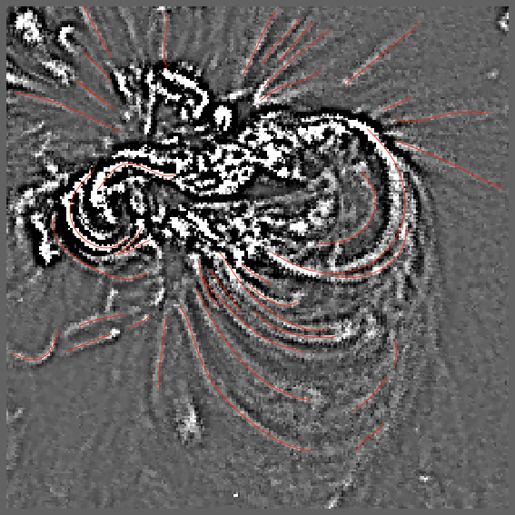
In the left part of Figure 6 we show the final fits obtained. For this result, the ridgels were found by automated scaling and interpolated by method (12), the parameters in (15) and (20) were $h_{\mathrm{max}}=3.0$ pixels, $r_{\mathrm{min}}=15.0$ pixels, and $a_{\mathrm{max}}=10.0$ degrees. The fits are represented by fifth degree parametric polynomials.

Obviously, the image processing cannot easily distinguish between structures which are due to moss and bright surface features and coronal loops. Even the observer is sometimes misled and there are no rigorous criteria for this distinction. Roughly, coronal loops produce longer and smoother fit curves, but there is no strict threshold because it may appear that the fit curve is split along a loop where the loop signal becomes faint. As a rule of thumb, a restriction to smaller curvature by choosing a higher parameter $r_{\mathrm{max}}$ and discarding shorter fit curves tends to favour coronal loops. Eventually, however, loops are suppressed, too. We have therefore appended a user interactive tool as the last step of our processing which allows us to eliminate unwanted curves, merge or split curves when smooth fits result with an energy (20) of the output fits not much higher than the energy of the input. The left part of Figure 6 shows the result of such a cleaning step.

References

- Alissandrakis (1981) Alissandrakis, C.E.: 1981, On the computation of constant alpha force-free magnetic field. A&A 100, 197 – 200.
- Aschwanden et al. (2007) Aschwanden, M., Gary, G.A., Smith, M., Inhester, B., Schrijver, K., DeRosa, M.: 2007, Automated tracing of coronal loops. Solar Phys., in press.
- Berger et al. (1999) Berger, T., De Pontieu, B., Fletcher, L., Schrijver, C., Tarbell, T., Title, A.: 1999, What is moss. Solar Phys. 190, 409 – 418.
- Carcedo et al. (2003) Carcedo, L., Brown, D.S., Hood, A.W., Neukirch, T., Wiegelmann, T.: 2003, A Quantitative Method to Optimise Magnetic Field Line Fitting of Observed Coronal Loops. Solar Phys. 218, 29 – 40.
- Dimas, Scholz, and Obermayer (2002) Dimas, A., Scholz, M., Obermayer, K.: 2002, Automatic segmentation and skeletonization of neurons from confocal microscopy images based on the 3d wavelet transform. IEEE Transactions on Image Processing 11(7), 790 – 801.
- Feng et al. (2007) Feng, L., Wiegelmann, T., Inhester, B., Solanki, S., Gan, W.Q., Ruan, P.: 2007, Magnetic Stereoscopy of Coronal Loops in NOAA 8891. Solar Phys. 241, 235 – 249. doi:10.1007/s11207-007-0370-z.
- Howard et al. (2007) Howard, R., Moses, J., Vourlidas, A., Newmark, J., Socker, D., Plunckett, S., Korendyke, C., Cook, J., Hurley, A., Davila, J., Thompson, W., St.Cyr, O., Mentzell, E., Mehalick, K., Lemen, J., Wuelser, J., Duncan, D., Tarbell, T., Harrison, R., Waltham, N., Lang, J., Davis, C., Eyles, C., Halain, J., Defise, J., Mazy, E., Rochus, P., Mercier, R., Ravet, M.., Delmotte, F., Auchère, F., Delaboudinière, J., Bothmer, V., Deutsch, W., Wang, D., Rich, N., Cooper, S., Stephens, V., Maahs, G., Baugh, R., McMullin, D.: 2007, Sun Earth Connection Coronal and Heliospheric Investigation. Adv. Space Res., in press.
- Inhester (2006) Inhester, B.: 2006, Stereoscopy basics for the STEREO mission. Int. Space Sci. Inst., submitted.(astro-ph/0612649)
- Inhester and Wiegelmann (2006) Inhester, B., Wiegelmann, T.: 2006, Nonlinear Force-Free Magnetic Field Extrapolations: Comparison of the Grad Rubin and Wheatland Sturrock Roumeliotis Algorithm. Solar Phys. 235, 201 – 221.
- Jang and Hong (2002) Jang, J.H., Hong, K.S.: 2002, Detection of curvilinear structures and reconstruction of their regions in grey scale images. Pattern Recognition 35, 807 – 824.
- Koller et al. (1995) Koller, T., Gerig, B., Székely, G., Dettwiler, D.: 1995, Multiscale detection of curvilinear structures in 2-d and 3-d image data. In: Proceedings Fifth Int. Conf. on Computer Vision (ICCV95). IEEE Computer Society Press, 864 – 869.
- Lee, Newman, and Gary (2006) Lee, J.K., Newman, T.S., Gary, G.A.: 2006, Oriented connectivity-based method for segmenting solar loops. Pattern Recognition 39, 246 – 259.
- Lindeberg (1998) Lindeberg, T.: 1998, Edge detection and ridge detection with automatic scale selection. International Journal of Computer Vision 30(2), 117 – 154.
- Medioni, Tang, and Lee (2000) Medioni, G., Tang, C.K., Lee, M.S.: 2000, Tensor voting: Theory and applications. http://citeseer.ist.psu.edu/medioni00tensor.html.
- Nguyen, Worring, and van den Boomgaard (2000) Nguyen, H., Worring, M., van den Boomgaard, R.: 2000, Watersnakes: Energy-driven watershed segmentation. http://citeseer.ist.psu.edu/article/nguyen00watersnakes.html.
- Parent and Zucker (1989) Parent, P., Zucker, S.: 1989, Trace inference, curvature consistency and curve detection. IEEE Transactions on Pattern Analysis and Machine Intelligence 11, 823 – 839.
- Seehafer (1978) Seehafer, N.: 1978, Determination of constant alpha force-free solar magnetic fields from magnetograph data. Solar Phys. 58, 215 – 223.
- Starck, Donoho, and Candès (2003) Starck, J.L., Donoho, D.L., Candès, E.J.: 2003, Astronomical image representation by the curvelet transform. A&A 398, 785 – 800.
- Steger (1998) Steger, C.: 1998, An unbiased detector of curvilinear structures. IEEE Transactions on Pattern Analysis and Machine Intelligence 20(2), 113 – 125.
- Taylor (1974) Taylor, J.B.: 1974, Relaxation of Toroidal Plasma and Generation of Reverse Magnetic Fields. Phys. Rev. Lett. 33, 1139 – 1141.
- Wiegelmann (2004) Wiegelmann, T.: 2004, Optimization code with weighting function for the reconstruction of coronal magnetic fields. Solar Phys. 219, 87 – 108.
- Wiegelmann et al. (2005) Wiegelmann, T., Lagg, A., Solanki, S.K., Inhester, B., Woch, J.: 2005, Comparing magnetic field extrapolations with measurements of magnetic loops. A&A 433, 701 – 705.
- Zhang and Yan (2004) Zhang, Q., Yan, H.: 2004, Fingerprint classification based on extraction and analysis of singularities and pseudo ridges. Pattern Recognition 37, 2233 – 2243.