Gradient flow approach to geometric convergence analysis of preconditioned eigensolvers Thanks: Received by the editors June 16, 2008; revised March 5, 2009; accepted March 16, 2009; published electronically ???????, 2009. Preliminary version http://arxiv.org/abs/0801.3099
Abstract
Preconditioned eigenvalue solvers (eigensolvers) are gaining popularity, but their convergence theory remains sparse and complex. We consider the simplest preconditioned eigensolver—the gradient iterative method with a fixed step size—for symmetric generalized eigenvalue problems, where we use the gradient of the Rayleigh quotient as an optimization direction. A sharp convergence rate bound for this method has been obtained in 2001–2003. It still remains the only known such bound for any of the methods in this class. While the bound is short and simple, its proof is not. We extend the bound to Hermitian matrices in the complex space and present a new self-contained and significantly shorter proof using novel geometric ideas.
keywords
iterative method; continuation method; preconditioning; preconditioner; eigenvalue; eigenvector; Rayleigh quotient; gradient iteration; convergence theory; spectral equivalenceAMS
49M37 65F15 65K10 65N25(Place for Digital Object Identifier, to get an idea of the final spacing.)
1 Introduction
We consider a generalized eigenvalue problem (eigenproblem) for a linear pencil with symmetric (Hermitian in the complex case) matrices and with positive definite . The eigenvalues are enumerated in decreasing order and the denote the corresponding eigenvectors. The largest value of the Rayleigh quotient where denotes the standard scalar product, is the largest eigenvalue . It can be approximated iteratively by maximizing the Rayleigh quotient in the direction of its gradient, which is proportional to . Preconditioning is used to accelerate the convergence; see, e.g., [2, 4, 5, 6, 8] and the references therein. Here we consider the simplest preconditioned eigenvalue solver (eigensolver)—the gradient iterative method with an explicit formula for the step size, cf. [2], one step of which is described by
| (1) |
The symmetric (Hermitian in the complex case) positive definite matrix in (1) is called the preconditioner. Since and are both positive definite, we assume that
| (2) |
The following result is proved in [8, 9, 10] for symmetric matrices in the real space.
Theorem 1.
If then and
| (3) |
The convergence factor cannot be improved with the chosen terms and assumptions.
Compared to other known non-asymptotic convergence rate bounds for similar preconditioned eigensolvers, e.g., [1, 2, 4, 5], the advantages of (3) are in its sharpness and elegance. Method (1) is the easiest preconditioned eigensolver, but (3) still remains the only known sharp bound in these terms for any of preconditioned eigensolvers. While bound (3) is short and simple, its proof in [8] is quite the opposite. It covers only the real case and is not self-contained—in addition it requires most of the material from [9, 10]. Here we extend the bound to Hermitian matrices and give a new much shorter and self-contained proof of Theorem 1, which is a great qualitative improvement compared to that of [8, 9, 10]. The new proof is not yet as elementary as we would like it to be; however, it is easy enough to hope that a similar approach might be applicable in future work on preconditioned eigensolvers.
Our new proof is based on novel techniques combined with some old ideas of [3, 9, 10]. We demonstrate that, for a given initial eigenvector approximation , the next iterative approximation described by (1) belongs to a cone if we apply any preconditioner satisfying (2). We analyze a corresponding continuation gradient method involving the gradient flow of the Rayleigh quotient and show that the smallest gradient norm (evidently leading to the slowest convergence) of the continuation method is reached when the initial vector belongs to a subspace spanned by two specific eigenvectors, namely and . This is done by showing that Temple’s inequality, which provides a lower bound for the norm of the gradient , is sharp only in . Next, we extend by integration the result for the continuation gradient method to our actual fixed step gradient method to conclude that the point on the cone, which corresponds to the poorest convergence and thus gives the guaranteed convergence rate bound, belongs to the same two-dimensional invariant subspace . This reduces the convergence analysis to a two-dimensional case for shifted inverse iterations, where the sharp convergence rate bound is established.
2 The proof of Theorem 1
We start with several simplifications:
Theorem 2.
We can assume that , , is diagonal, eigenvalues are simple, , and in Theorem 1 without loss of generality.
Proof.
First, we observe that method (1) and bound (3) are evidently both invariant with respect to a real shift if we replace the matrix with , so without loss of generality we need only consider the case which makes Second, by changing the basis from coordinate vectors to the eigenvectors of we can make diagonal and . Third, having if or , or both, bound (3) becomes trivial. The assumption is a bit more delicate. The vector depends continuously on the preconditioner , so we can assume that and extend the final bound to the case by continuity.
Finally, we again use continuity to explain why we can assume that all eigenvalues (in fact, we only need and ) are simple and make and thus without changing anything. Let us list all -dependent terms, in addition to all participating eigenvalues, in method (4): and ; and in bound (3): and . All these terms depend on continuously if is slightly perturbed into with some , so we increase arbitrarily small the diagonal entries of the matrix to make all eigenvalues of simple and . If we prove bound (3) for the matrix with simple positive eigenvalues, and show that the bound is sharp as with , we take the limit and by continuity extend the result to the limit matrix with and possibly multiple eigenvalues. ∎
It is convenient to rewrite (1)–(3) equivalently by Theorem 2 as follows11 1 Here and below denotes the Euclidean vector norm, i.e., for a real or complex column-vector , as well as the corresponding induced matrix norm.
| (4) | |||
| (5) |
and if and then and
| (6) |
Now we establish the validity and sharpness of bound (6) assuming (4) and (5).
Theorem 3.
Let us define22 2 We define angles in between vectors by . then and . Let be defined as the vector constrained by and with the smallest value . Then .
Proof.
Orthogonality by the Pythagorean theorem implies , so , since as , and where as . A ball with the radius by (5) centered at contains by (4), so .
The statement follows directly from the definition of . Now,
as , so and ∎
We denote by the circular cone around with the opening angle . Theorem 3 replaces with the minimizer of the Rayleigh quotient on the cone in the rest of the paper, except at the end of the proof of Theorem 8, where we show that bounding below the value instead of still gives the sharp estimate.
Later on, in the proof of Theorem 5, we use an argument that holds easily only in the real space, so we need the following last simplification.
Theorem 4.
Without loss of generality we can consider only the real case.
Proof.
The key observation is that for our positive diagonal matrix the Rayleigh quotient depends evidently only on the absolute values of the vector components, i.e., , where the absolute value operation is applied component-wise. Moreover, and , so . The cone lives in the complex space, but we also need its substitute in the real space. Let us introduce the notation for the real circular cone with the opening angle centered at the real vector Next we show that in the real space we have the inclusion .
For any complex nonzero vectors and , we have by the triangle inequality, thus . If then , i.e., indeed, , which means that as required.
Therefore, changing the given vector to take its absolute value and replacing the complex cone with the real cone lead to the relations , but does not affect the starting Rayleigh quotient This proves the theorem with the exception of the issue of whether the sharpness in the real case implies the sharpness in the complex case; see the end of the proof of Theorem 8. ∎
Theorem 5.
We have and such that . The inclusion implies
Proof.

Assuming that is strictly inside the cone implies that is a point of a local minimum of the Rayleigh quotient. The Rayleigh quotient has only one local (and global) minimum, , but the possibility is eliminated by Theorem 3, so we obtain a contradiction, thus .
The necessary condition for a local minimum of a smooth real-valued function on a smooth surface in a real vector space is that the gradient of the function is orthogonal to the surface at the point of the minimum and directed inwards. In our case, is a circular cone with the axis and the gradient is positively proportional to ; see Figure 1. We first scale the vector such that so that the vector is an inward normal vector for at the point . This inward normal vector must be positively proportional to the gradient, with , which gives , where . Here as otherwise would be an eigenvector, but by Theorem 3, where by assumptions , while by Theorem 2, which gives a contradiction. As the scaling of the minimizer is irrelevant, we denote here by with a slight local notation abuse.
Finally, since , inclusion gives either the required inclusion or with for some and We now show that the latter leads to a contradiction. We have just proved that , thus . Let , where we notice that and since is not an eigenvector. Then we obtain where , therefore . Since all eigenvalues are simple, We observe that , i.e., in the mapping of to the coefficient in front of changes by a smaller absolute value compared to the change in the coefficient in front of . Thus, using the monotonicity of the Rayleigh quotient in the absolute values of the coefficients of the eigenvector expansion of its argument, which contradicts proved in Theorem 3. ∎
Theorem 5 characterizes the minimizer of the Rayleigh quotient on the cone for a fixed . The next goal is to vary , preserving its Rayleigh quotient , and to determine conditions on leading to the smallest in such a setting. Intuition suggests (and we give the exact formulation and the proof later in Theorem 7) that the poorest convergence of a gradient method corresponds to the smallest norm of the gradient, so in the next theorem we analyze the behavior of the gradient of the Rayleigh quotient and the cone opening angle
Theorem 6.
Let be fixed and the level set of the Rayleigh quotient be denoted by . Both and with attain their minima on in
Proof.
By definition of the gradient, for . The Temple inequality is equivalent to the operator inequality , which evidently holds. The equality here is attained only for
Finally, we turn our attention to the angles. For the Pythagorean theorem shows that
is minimized together with . But for a fixed the function is strictly increasing in which proves the proposition for ∎
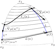
Now we are ready to show that the same subspace gives the smallest change in the Rayleigh quotient . The proof is based on analyzing the negative normalized gradient flow of the Rayleigh quotient.
Theorem 7.
Under the assumptions of Theorems 5 and 6 we denote —the set of minimizers of the Rayleigh quotient. Then (See Figure 2).
Proof.
The initial value problem for a gradient flow of the Rayleigh quotient,
| (7) |
has the vector-valued solution which preserves the norm of the initial vector since as . Without loss of generality we assume The Rayleigh quotient function is decreasing since
As , the function is strictly decreasing at least until it reaches as there are no eigenvalues in the interval but only eigenvectors can be special points of ODE (7). The condition thus uniquely determines for a given initial value . The absolute value of the decrease of the Rayleigh quotient along the path is
Our continuation method (7) using the normalized gradient flow is nonstandard, but its advantage is that it gives the following simple expression for the length of ,
Since the initial value is determined by , we compare a generic with the special choice , using the superscript to denote all quantities corresponding to the choice . By Theorem 5 implies , so we have as is an invariant subspace for the gradient of the Rayleigh quotient. At the end points, by their definition. Our goal is to bound the initial value by , so we compare the lengths of the corresponding paths and and the norms of the gradients along these paths.
We start with the lengths. We obtain by Theorem 6. Here the angle is the smallest angle between any two vectors on the cones boundaries and . Thus, as our one vector by Theorem 5, while the other vector cannot be inside the cone since by Theorem 3. As is a unit vector, as the angle is the length of the arc—the shortest curve from to on the unit ball.
For our special -choice, inequalities from the previous paragraph turn into equalities, as is in the intersection of the unit ball and the subspace , so the path is the arc between to itself. Combining everything together,
By Theorem 7 the poorest convergence is attained with and with the corresponding minimizer described in Theorem 5, so finally our analysis is now reduced to the two-dimensional space .
Theorem 8.
Bound (6) holds and is sharp for .
Proof.
Assuming and , we derive
| (8) |
and similarly for where .
Since , we have . Assuming , this identity implies which contradicts our assumption that is not an eigenvector. For and by Theorem 5, the inverse exists.
Next we prove that and that it is a strictly decreasing function of Indeed, using and our cosine-based definition of the angles, we have where We substitute , which gives Using (8), multiplication by leads to a simple quadratic equation, for As , , and , the discriminant is positive and the two solutions for , corresponding to the minimum and maximum of the Rayleigh quotient on , have different signs. The proof of Theorem 5 analyzes the direction of the gradient of the Rayleigh quotient to conclude that and correspond to the minimum. Repeating the same arguments with shows that corresponds to the maximum. But since , hence the negative corresponds to the maximum and thus the positive corresponds to the minimum. We observe that the coefficients and are evidently increasing functions of , while does not depend on . Thus is strictly decreasing in , and taking gives the smallest
Since where now , condition implies and implies so we introduce the convergence factor as
where we use (8) and again . We notice that is a strictly decreasing function of and thus takes its largest value for giving i.e., bound (6) that we are seeking.
The convergence factor cannot be improved without introducing extra terms or assumptions. But deals with , not with the actual iterate . We now show that for there exist a vector and a preconditioner satisfying (5) such that and in both real and complex cases. In the complex case, let us choose such that and according to (8), then the real vector is a minimizer of the Rayleigh quotient on , since and .
Finally, for a real with and a real properly scaled there is a real matrix satisfying (5) such that , which leads to (4) with Indeed, for the chosen we scale such that so . As vectors and are real and have the same length there exists a real Householder reflection such that . Setting we obtain the required identity. Any Householder reflection is symmetric and has only two distinct eigenvalues , so we conclude that is real symmetric (and thus Hermitian in the complex case) and satisfies (5). ∎
3 Appendix
The integration of inverse functions theorem follows.
Theorem 9.
Let for be strictly monotone increasing smooth functions and suppose that for we have . If for all with the derivatives satisfy then for any we have
Proof.
For any we have (using )
If , then for the derivatives of the inverse functions it holds that Since and are strictly monotone increasing functions the integrands are positive functions and as well as . Comparing the lower limits of the integrals gives the statement of the theorem. ∎
Conclusions
We present a new geometric approach to the convergence analysis of a preconditioned fixed-step gradient eigensolver which reduces the derivation of the convergence rate bound to a two-dimensional case. The main novelty is in the use of a continuation method for the gradient flow of the Rayleigh quotient to locate the two-dimensional subspace corresponding to the smallest change in the Rayleigh quotient and thus to the slowest convergence of the gradient eigensolver.
An elegant and important result such as Theorem 1 should ideally have a textbook-level proof. We have been trying, unsuccessfully, to find such a proof for several years, so its existence remains an open problem.
Acknowledgments
We thank M. Zhou of University of Rostock, Germany for proofreading. M. Argentati of University of Colorado Denver, E. Ovtchinnikov of University of Westminster, and anonymous referees have made numerous great suggestions to improve the paper and for future work.
REFERENCES
- [1] J. H. Bramble, J. E. Pasciak, and A. V. Knyazev, A subspace preconditioning algorithm for eigenvector/eigenvalue computation, Adv. Comput. Math., 6 (1996), pp. 159–189.
- [2] E. G. D’yakonov, Optimization in solving elliptic problems, CRC Press, 1996.
- [3] A. V. Knyazev, Computation of eigenvalues and eigenvectors for mesh problems: algorithms and error estimates, (In Russian), Dept. Num. Math., USSR Ac. Sci., Moscow, 1986.
- [4] A. V. Knyazev, Convergence rate estimates for iterative methods for a mesh symmetric eigenvalue problem, Russian J. Numer. Anal. Math. Modelling, 2 (1987), pp. 371–396.
- [5] A. V. Knyazev, Preconditioned eigensolvers—an oxymoron?, Electron. Trans. Numer. Anal., 7 (1998), pp. 104–123.
- [6] A. V. Knyazev, Preconditioned eigensolvers: practical algorithms, In Z. Bai, J. Demmel, J. Dongarra, A. Ruhe, and H. van der Vorst, editors, Templates for the Solution of Algebraic Eigenvalue Problems: A Practical Guide, pp. 352–368. SIAM, Philadelphia, 2000.
- [7] A. V. Knyazev, Toward the optimal preconditioned eigensolver: Locally optimal block preconditioned conjugate gradient method, SIAM J. Sci. Comput., 23 (2001), pp. 517–541.
- [8] A. V. Knyazev and K. Neymeyr, A geometric theory for preconditioned inverse iteration. III: A short and sharp convergence estimate for generalized eigenvalue problems, Linear Algebra Appl., 358 (2003), pp. 95–114.
- [9] K. Neymeyr, A geometric theory for preconditioned inverse iteration. I: Extrema of the Rayleigh quotient, Linear Algebra Appl., 322 (2001), pp. 61–85.
- [10] K. Neymeyr, A geometric theory for preconditioned inverse iteration. II: Convergence estimates, Linear Algebra Appl., 322 (2001), pp. 87–104.