Protostellar collapse: A comparison between SPH and AMR calculations.
Abstract
Context. The development of parallel supercomputers allows today the detailed study of the collapse and the fragmentation of prestellar cores with increasingly accurate numerical simulations. Thanks to the advances in sub-millimeter observations, a wide range of observed initial conditions enable us to study the different modes of low-mass star formation. The challenge for the simulations is to reproduce the observational results.
Aims. Two main numerical methods, namely AMR and SPH, are widely used to simulate the collapse and the fragmentation of prestellar cores. We compare thoroughly these two methods within their standard framework.
Methods. We use the AMR code RAMSES and the SPH code DRAGON. Our physical model is as simple as possible, and consists of an isothermal sphere rotating around the -axis. We first study the conservation of angular momentum as a function of the resolution. Then, we explore a wide range of simulation parameters to study the fragmentation of prestellar cores.
Results. There seems to be a convergence between the two methods, provided resolution in each case is sufficient. Resolution criteria adapted to our physical cases, in terms of resolution per Jeans mass, for an accurate description of the formation of protostellar cores are deduced from the present study. This convergence is encouraging for future work in simulations of low-mass star formation, providing the aforementioned criteria are fulfilled.
Key Words.
Stars: formation - Methods : numerical - hydrodynamics1 Introduction
Star formation is known for being the place of extreme variations in length and density scales. Although it is established that stars form in dense cores, the non-linear evolution makes it difficult to perform accurate calculations of the collapse and the fragmentation of a prestellar core. The star formation process is the outcome of complex gas dynamics involving non-linear interactions of gravity, turbulence, magnetic field and radiation. Early theoretical pioneer works by Larson (1969), Penston (1969) or Shu (1977) are among the many illustrations of the high complexity of the gravitational collapse. Recently, Klein et al. (2007) pointed out that developing a theory for low-mass star formation remains one of the most elusive and important goals of theoretical astrophysics. The computational challenge stems from the fact that star formation occurs in clouds over many orders of magnitude in spatial and density scales. Following the gravitational collapse while resolving precisely the Jeans length, which scales as for an isothermal gas, is a major difficulty for numerical simulations.
Different approaches are used to study star formation through numerical simulations and include more and more detailed physics. One key question resides in the validation of the numerical methods used to study low-mass star formation. Nowadays, two completely different numerical method are used with sufficient accuracy:
- 1.
AMR: Adaptive Mesh Refinement method for Eulerian grids
- 2.
SPH: Smoothed Particle Hydrodynamics method for a Lagrangian approach.
No systematic comparison between the two methods has been done with low-mass star formation calculations. However, a lot of numerical works have been carried out and some of them are common test calculations for convergence testing and intercode comparisons. The most famous model was first calculated by Boss & Bodenheimer (1979) and since then, it has been recalculated by several authors with even higher spatial resolution (Bate & Burkert, 1997; Truelove et al., 1998; Kitsionas & Whitworth, 2002; Arreaga-García et al., 2007, e.g). The SPH approach has generated a lot of detailed investigations on the influence of the number of particles and neighbors (Lombardi et al., 1999; Rasio, 1999; Attwood et al., 2007), and criteria for numerical convergence have been extracted from these studies. Nelson (2006) performed a large investigation of the influence of these parameters on disk fragmentation, and concluded that the better the resolution the later the fragmentation. Dehnen (2001) investigated the optimal gravitational force softening necessary in three-dimensional -body codes. Bate & Burkert (1997) provide a minimum resolution criterion for SPH calculations with self-gravity to accurately model fragmentation. Less studies have been performed with AMR since AMR codes have become available recently. Truelove et al. (1997) give an empirical criterion for the Jeans length resolution in AMR calculations to avoid spurious numerical fragmentation.
There are not much of direct comparison between SPH and AMR
calculations. Comparison in the context of cosmological simulations
has been done through the Santa Barbara Cluster Comparison Project
(Frenk et al., 1999). Fromang et al. (2006) compares quite
successfully AMR hydrodynamical collapse calculations with the ones of
Hosking & Whitworth (2004), using the SPH method.
In the present paper, we compare thoroughly the two approaches in the context of low-mass prestellar core formation. We stress that the main goal of this paper is to investigate whether convergence can be achieved between the two methods. We have conducted calculations over a wide range of numerical resolution parameters, in order to study the dependency of angular momentum conservation and fragmentation on physical and numerical initial conditions. We then derive resolution criteria necessary to describe accurately prestellar core formation.
The paper is organized as follows: in §2 we briefly introduce our
collapse model. In §3, we present the two codes used for our
comparative study as well as our initial numerical conditions and the
criteria we fulfill to resolve gravitational collapse. The problem of
angular momentum conservation is examined in detail §4. In §5, we
tackle the fragmentation issue and explore the dependency of the
results on the numerical parameters. First, we study the numerical
convergence of AMR and SPH calculations separately. Then, we compare
the respective converged calculations. This convergence study is done
for different test cases. In section 6 we conclude this paper by
deriving for each method empirical required numerical criteria for an
accurate description of gravitational collapse and fragmentation
adapted to our test cases.
The convention in this paper is to call "particles" the SPH particles and "cells" the AMR cells in order to avoid confusion.
2 Definitions of the test cases
2.1 Model
To make comparison between codes easier, we adopt simple initial conditions, similar to those chosen in previous studies (Boss & Bodenheimer, 1979; Bate & Burkert, 1997, e.g.). We consider an uniform-density sphere of molecular gas of initial radius , rotating around the -axis with an uniform angular velocity , in order to minimize the loss of angular momentum due to friction. We fix the cloud mass at M☉ and the temperature at 10 K. For a mixture of molecular hydrogen, helium and heavy elements, this corresponds to an isothermal sound speed of km.s-1. For the case where fragmentation occurs, we use a azimuthal density perturbation.
The initial energy balance of our model is determined by two dimensionless parameters corresponding to the ratio between the thermal energy and the gravitational energy
| (1) |
and to the ratio of the rotational and the gravitational energy
| (2) |
Since we use a constant initial mass of 1 M☉ and a constant temperature, changing one of the two parameters, namely , gives the sphere radius . The higher , the larger . The angular velocity is given by the parameter .
2.2 The barotropic equation of state
In order to mimic the thermal behaviour of a star-forming gas, we use a barotropic equation of state (Bonnell, 1994, cf.). Tohline (1982) and Masunaga & Inutsuka (2000) showed that the core follows closely a barotropic equation of state, providing a good approximation without resolving radiative transfer. We use
| (3) |
where is the sound speed and g.cm-3 is the critical density which corresponds to the transition from an isothermal to an adiabatic state (Larson, 1969).
At low densities, , km.s-1. The molecular gas is able to radiate freely by coupling thermally to the dust and therefore remains isothermal at 10 K. At high densities , we assume that the cooling due to radiative transfer is trapped by the dust opacity. Therefore, which corresponds to an adiabatic monoatomic gas with adiabatic exponent . Note that molecular hydrogen behaves like a monoatomic gas until the temperature reaches several hundred Kelvin, since the rotational degrees of freedom are not excited at lower temperatures, and hence is the appropriate adiabatic exponent (Whitworth & Clarke, 1997; Masunaga & Inutsuka, 2000).
3 Numerical methods and initial conditions
3.1 AMR: Adaptive Mesh Refinement
3.1.1 A brief history
The Adaptive Mesh Refinement method is one of the most promising numerical methods to solve the fluid equations. The technique was first introduced in Berger & Oliger (1984). Originally, the AMR method was an Eulerian hydrodynamical scheme, with a hierarchy of nested grids covering high resolution regions of the flow. This first AMR structure, called “patch-based AMR”, consists of building blocks of the computational grid as rectangular patches of various sizes. An alternative method was proposed (Khokolov, 1998, i.e.), the “tree-based” AMR, where the parent cells are refined into children cells on a cell-by-cell basis. These adaptive mesh structures are coupled with grid-based fluid dynamics schemes handling high-resolution shock capturing. Nowadays, high order Godunov methods appear to be amongst the best schemes to capture discontinuities within only a few cells (Teyssier, 2002; Matsumoto & Hanawa, 2003; Ziegler, 2005; Fromang et al., 2006, e.g.).
3.1.2 The RAMSES code
In this paper, we use the AMR code RAMSES (Teyssier, 2002), which
integrates the “tree-based” data structure allowing recursive grid
refinements. RAMSES uses a second order Godunov hydrodynamical scheme
coupled with a gravity solver. Furthermore, it has the possibility to
use variable timesteps at each refinement level. Concerning time
integration, RAMSES uses a second-order midpoint scheme, where
positions and velocities are updated by a predictor-corrector step.
Recently, an ideal MHD version of RAMSES has been developed by
Fromang et al. (2006).
The Godunov hydrodynamical solver is able to capture discontinuities with a high precision level. The equations solved in RAMSES are the Euler equations in their conservative form
| (4) |
| (5) |
| (6) |
where is the gas pressure ( is the identity matrix), the density, u the velocity, the total energy density and the gravitational potential. The system of equations is closed with the barotropic equation of state (3).
One of the main advantages of solving the Euler equations in their conservative form is that no energy sink due to numerical errors can alter the flow dynamics (ignoring the source terms due to gravity). Equations 4, 5 and 6 are solved with a Lax-Friedrich Riemann solver, known to be one of the most simple and robust scheme. In Appendix C, we report on the influence of using the Roe solver which is less diffusive but considerably more complex and numerically expensive.
The timestep is determined independently for each refinement level , using standard stability constraints for the hydrodynamical solver. Each level evolves according to its own timestep.
3.1.3 Initial conditions for RAMSES
One practical limitation of AMR codes is the use of Cartesian grids. RAMSES works with a cubic volume, so that a part of the calculation box is lost when we describe a sphere. The outer region of the sphere is also at a 10 K temperature but is 100 times less dense. Therefore, the outer gas has no effect on the dynamics of the sphere since the two parts are well separated. The sphere radius is equal to a quarter of the box length in order to minimize border effects.
3.2 SPH: Smoothed Particles Hydrodynamics
3.2.1 A brief overview
SPH is the most popular fully Lagrangian method used to describe gravitational collapse because of its simplicity for 3D codes and its versatility to incorporate self-gravity. SPH was first designed to simulate nonaxisymmetric phenomena for astrophysical gases (Lucy, 1977; Gingold & Monaghan, 1977). This method is easy to work with and can give rapidly reasonably accurate results. SPH is economic in handling hydrodynamical flows that have near empty regions. It does not need a grid to calculate spatial derivatives, but consists of a set of discrete particles describing the state of the fluid. The spatial derivatives are found by analytical differentiation of interpolation formulae. SPH particle should not be perceived as a real fluid element, but as a mathematical entity with coordinates , velocity , mass (i.e. since all particles have the same mass in the present calculations) and thermal energy . The evolution of the fluid is determined by following the motion of the particles, under the influence of interparticle forces which represent the effects of pressure, viscosity (see below) and self-gravity.
The main advantage of SPH is its strict Galilean-invariant property and its simplicity. Resolution elements are then concentrated in high density regions in SPH methods . The standard SPH formalism uses artificial viscosity for the hydrodynamics. Some alternative formalism such as Godunov SPH has been proposed (Inutsuka, 1994, e.g.) in order to avoid the use of artificial viscosity, but these methods are not yet mature. SPH has been used by several authors to study fragmentation (Bonnell, 1994; Bate & Burkert, 1997; Goodwin et al., 2004; Hennebelle et al., 2004).
3.2.2 Hydrodynamical method for DRAGON
We use the standard SPH code DRAGON (Turner et al., 1995; Goodwin et al., 2004), i.e in its most simple version. In standard SPH, the integral interpolant for the variable is approximated by a summation interpolation over the particle’s nearest neighbors:
| (7) |
where is the value associated with particle , and is the adaptive smoothing length of particle , defined such that the particle kernel volume contains a constant mass, i.e. a constant number of neighbors . The interpolation mass is then given by .
We use a standard artificial viscosity scheme (Gingold & Monaghan, 1983):
| (8) |
with
| (9) |
where , and and denote arithmetic means of the isothermal sound speed and density of the particles and . The free parameters , and regulate the strength of the viscosity. In our case, we have the combination , and . This artificial viscosity is the subject of several discussions where authors suggest alternative artificial viscosity. One common improvement is to use a time-dependent viscosity (Morris & Monaghan, 1997). We look at the influence of the viscosity scheme in Appendix B.
The gravitational force between a pair of particles obeys a simple inverse-square law, unless the particles are very close. Under this circumstance, the gravity force has to be softened to avoid violent two-body interaction. According to Bate & Burkert (1997), the gravitational softening length should be the same as the hydrodynamic smoothing length. Calculation of the gravitational acceleration of an SPH particle is speeded up using an octal Spatial Tesselation Tree (STT) (Hernquist, 1987) and accounts for the quadrupole moments of the mass distributions. DRAGON benefits from the implementation of “sink particles” creation (Bate et al., 1995), used to continue the calculations without resolving processes on extremely short time-scales. Last but not least, DRAGON uses multiple-particle timesteps.
Finally, we allow a variation of the number of neighbors less than 10% of in our SPH calculations, i.e when . Attwood et al. (2007) shows that the smaller , the less diffusive is SPH. Ideally, should be set to 0. We report on the influence of setting for local angular momentum conservation in Appendix B.
3.2.3 Initial conditions for DRAGON
We use the method originally presented by Whitworth et al. (1995) to obtain an initial particle distribution which consist in settling the positions of the particles randomly settled by using only hydrodynamical forces over a few timesteps. Another approach sometimes used is to take initial hexagonal-close-paced lattice of SPH particles to generate initial conditions. However, standard SPH calculations start from noisy initial particle distributions at present time (Arreaga-García et al., 2007, e.g.). Note that we do not need intercloud and external particles to confine the ones within the sphere since our model is initially far from equilibrium.
3.3 The Jeans criterion in numerical codes
3.3.1 Refinement criterion for the AMR method
Our refinement criterion is based on the Jeans length resolution which is necessary to treat accurately gravitational collapse. We impose a minimum number of points per Jeans length . The cells’ dimensions must be smaller than a constant fraction of the local Jeans length. The dimension of cells belonging to the refinement level is , where is the physical length of the simulation box. The mesh is locally refined in order to satisfy the local Jeans criterion:
| (10) |
Truelove et al. (1997) defined a minimum resolution condition for the validity of grid-based simulations aimed at modeling the collapse of a molecular cloud core, namely . This condition ensures that the collapse is of physical rather than of numerical origin.
3.3.2 Jeans length description with a SPH code
In standard SPH, the resolution in mass is fixed and thus the Jeans length resolution deteriorates with increasing density for an isothermal gas. The minimum resolvable mass must then be larger than the interpolation mass. Bate & Burkert (1997) showed that the behaviour of a Jeans-mass clump of gas with radius is dominated by the numerical implementation. Bate & Burkert (1997) take the smallest mass that can be resolved in SPH calculations to be equal to the mass of particles. According to this criterion, we can determine an initial number of SPH particles necessary to solve the Jeans length in the simulations.
The Jeans mass is and the minimum resolvable mass is . Hence, we can define a Jeans condition corresponding to the minimum value of , given by the barotropic equation of state (3), i.e. :
| (11) |
Considering an initial spherical mass M☉, the initial number of particles has to satisfy if . This is the critical number of particles used in SPH calculations to study the collapse of a dense core. We have in that case exactly (i.e. two resolution elements) particles per critical Jeans mass. Hubber et al. (2006) shows that with this numerical resolution, standard SPH will capture fragmentation which is genuine and resolved.
As mentioned before, the mass resolution is fixed in standard SPH. In term of Jeans mass, the resolution is therefore high at the beginning of the simulation and decreases when the density increases up to the critical density. It is nevertheless instructive to have a means of comparing the SPH and AMR resolution. We therefore define for the SPH the parameter such that is the number of resolution element per Jeans mass. This number is computed at the critical density , i.e. the most unfavorable case for the SPH. In the dense core where , the parameter enables us to compare the resolution achieved by SPH and AMR, respectively. Using particle splitting refinement in SPH (Kitsionas & Whitworth, 2002, e.g.) would improve its resolution. Indeed, particle splitting is an economic way to increase the local resolution and thus to avoid violating the Jeans condition in collapse simulations. However, as mentioned in the introduction, the aim of the present paper is to compare the AMR and the SPH within their standard implementation.
4 Free-fall time and angular momentum conservation
We start by comparing the global properties of the collapse in the two codes in the simple case of an uniform-density sphere collapse with no perturbation. We look at the collapse time, the accretion shock and finally the angular momentum conservation.
We carried out a first set of simulations within a wide range of resolution parameters. The initial sphere is set up by parameters corresponding to an initial radius cm and a density g.cm-3. The corresponding free-fall time is t kyr.
|


4.1 Free-fall time
The first step is to compare the calculations collapse time when the initial sphere is not rotating (i.e. ). Note that since is large and since we use a barotropic equation of state, we expect to find a value larger than the free-fall time. Then, we use as a reference time t t for which . Table 1 gives collapse times t0 as a function of resolution parameters for AMR and SPH calculations. AMR calculations have been run with and and 7, SPH calculations with ranging from to and a number of neighbors . We note that with , we do not satisfy the Bate & Burkert (1997) criterion, but the mass of our resolution element, i.e. the sphere containing the neighbors, is smaller that the critical Jeans mass.
With increasing numerical resolution, the numerical time t0 decreases and seems to converge toward a value slightly greater than the free-fall time. Time t0 changes by less than 5% between AMR calculations with and 7 and SPH calculations with and . Dynamical times t0 in SPH calculations are closer to the free-fall time than the AMR ones. This is partly due to the higher initial resolution in SPH.
4.1.1 Collapse and accretion shock with rotation
The gas sphere is now in solid rotation around the -axis. We set , corresponding to an orbital time t kyr. Table 2 summarizes the different SPH and AMR calculations run for this case. In order to illustrate the core resolution, we give the quantity representing the number of cells/particles with density g.cm-3 at t0. AMR simulations have been performed with different minimum refinement levels ranging from 5 to 7 and a refinement criterion ranging from 4 to 10. As expected, at a constant , the various AMR calculations show a convergence. The SPH simulations were performed with a constant number of neighbors and a total number of particles ranging from to . A consequence of the deteriorating resolution with increasing density in standard SPH, as mentioned earlier, is illustrated by the fact that, for equivalent initial condition, it is easier to get a better core resolution with AMR.
In Fig.1(a) we show density profiles as a function of the radius in the equatorial plane for AMR calculations with and and for the SPH with and . The density profiles are very similar, indicating good convergence between the two methods. The behaviour differs at relatively high radius because of the external gas in the AMR method. In the present simulations, the dynamical time to reach is increased by kyr, because of the rotational support. As seen in Table 2, when one increases the resolution, one seems to converge toward this time.

When the core becomes adiabatic, the angular momentum conservation induces the formation of an accretion disk around the central object. The centrifugal force becomes comparable to the gravitational one on the equatorial plane, slowing down the collapse. The outer collapsing gas, which has a supersonic infalling speed, meets suddenly the static gas of the core, creating an accretion shock. This shock can be clearly seen in Fig. 1(b) where the radial velocity component averaged over the equatorial plane is displayed. The accretion shock is described slightly more accurately with the AMR method. The SPH curve is smoother before the shock due to the artificial viscosity scheme. The slope before the shock strongly depends on the hydrodynamical solver so the results illustrate the difference between the hydrodynamical methods used in our two codes.
4.2 Theoretical local angular momentum
We now investigate the issue of angular momentum conservation. Note that both SPH and AMR equations ensure conservation of the linear momentum. Considering our axisymmetric model, without azimuthal perturbation, we can easily investigate the effect of numerical resolution on angular momentum conservation. The local angular momentum should be well conserved, until azimuthal symmetry is broken. The loss of local angular momentum in our model is only due to unphysical transport inherent to the numerical methods used in the two codes. Thanks to its Lagrangian properties, the SPH calculations gives access to the angular momentum that each particle has initially, i.e. the angular momentum that particle should have if the numerical scheme was conserving it exactly. Having access to the particle initial angular momentum, the loss of angular momentum is easily calculated. The azimuthal velocity component, directly linked to the angular momentum , is given by
| (12) |
where is the distance from the rotation axis
| (13) |
and the angular momentum
| (14) |
The angular momentum conservation along the -axis allows us to write
| (15) |
Thus, the theoretical angular velocity of a particle at time is determined by the ratio between its initial angular momentum and its actual radius:
| (16) |
With Eq. (16), we can compare the theoretical angular velocity component to the numerical ones, and in particular with the AMR results for which we do not have access to a theoretical value. Since SPH and AMR density profiles are almost identical at t0, we suppose that the previous mapping giving as a function of the radius in the SPH runs is also valid for the AMR calculations. Note also that the method cannot account for the displacement of the particles which would arise by changing the angular momentum.
4.2.1 Azimuthal velocity component
Figure 2 gives the ratio between the angular momentum and for the SPH simulation with and . The particles are ordered in decreasing density and the ratio is averaged over particles. A first interesting result is that denser particles loose more angular momentum. At tff, denser particles have lost 3% of their initial angular momentum. In less resolved calculations, i.e. particles, the effect is stronger and the densest ones loose more than 10% of their initial angular momentum in a free-fall time tff. This percentage slightly decreases when increasing the number of particles. The reason is that the denser the particle the larger the viscous torque (see below) and thus the larger the angular momentum transport. This numerical transport is amplified when the core is close to becoming adiabatic.
Figure 3 shows the cumulated hydrodynamical (left-hand side) and viscous (right-hand side) torques on the rotational axis for the same SPH calculations at the same times as in Fig. 2. In principle, there should not be any torque on the rotational axis because of this axisymmetric model. The cumulated torques are computed and summed at each timestep for each particle. The value plotted is an average over 7 500 particles and particles are ordered in decreasing density. Denser particles have the largest cumulated hydrodynamical and viscous torques. The friction forces corresponding to the hydrodynamical torque are stronger for these particles, which is due to the strong differential velocity.


| ||||||||||||||||||||||||||||||||||||
|
Figure 4a displays the azimuthal velocity component as a function of the radius on the -plane for the SPH simulations. The theoretical azimuthal velocity profile (solid line) is obtained following the previous section. It is obvious that low resolution simulations are not able to conserve properly the angular momentum. With particles, we obtain counter-rotating particles at the center (not illustrated in Fig. 4a because of the average in the -plane that smoothes the profiles). It appears that a minimum of particles is required to maintain angular momentum loss within less than , for the case of the present study. The improvement of angular momentum conservation eventually saturates for large numbers of particles. We checked that using a larger number of neighbors does not improve the conservation of local angular momentum.
Figure 4b shows results obtained with the RAMSES code. AMR curves are plotted and compared with the theoretical one obtained previously for SPH. The simulations with and are close to the theoretical curve. In both AMR simulations with , dense core resolution is higher than with SPH. For an initial resolution of =5, the AMR scheme does produce some angular momentum lag. This can be due to the fact that with a poor initial resolution, the interpolation of the gravitational potential tends to convert gravitational energy into rotational energy. The outer gas does not alter the angular momentum conservation for AMR calculations because of its tiny density.


In Fig. 5a,b, we plot the integrated mass and the ratio of numerical over theoretical angular momentum for AMR calculations with , and for SPH calculations with , . In Fig. 5a, most of the mass of the forming disk remains within a radius cm, i.e. where AMR and SPH have an opposite behaviour. In Fig. 5b, angular momentum is clearly transported to the outer regions with SPH, whereas it has a slight trend to be transported to the inner regions with the AMR. The overall angular momentum is well conserved in both calculations, but local properties seem to be affected by initial resolution. SPH resolution is much better at the beginning of the calculations, which enables SPH to properly conserve local angular momentum at cm at t0 while low initial resolution of the sphere in AMR induces a worse conservation. This effect reverses at lower radius where AMR can reach smaller scales contrary to standard SPH.
The density profiles obtained with the two methods converge towards a similar solution (c.f. Fig.1a) but a closer analysis of the velocity profiles shows discrepancies. We can say that angular velocity profiles indicate that local angular momentum is better conserved with the AMR than with the SPH method for the code implementation that we used. Both can be improved using appropriate methods (see appendix B and C).
5 Fragmentation
5.1 Model
Prestellar core fragmentation is a highly non-linear process. A key issue is to understand to what extent the fragmentation which occurs in numerical simulations is influenced by the numerical scheme and resolution.

To study dense core fragmentation, we choose the same previous spherical model and impose a azimuthal density perturbation:
| (17) |
where is the mean sphere density, the perturbation
amplitude and the azimuthal angle in cylindrical coordinates.
The initial conditions are easy to implement for the AMR calculations. The SPH sinusoidal density perturbation is imposed by adjusting the unperturbed -coordinate of each particle to a perturbed value given by:
| (18) |
We compare simulations for three different thermal supports, namely , 0.5 and 0.65, with a fixed rotational support . In the following, the convention is to call fragments the clumps where the gas density satisfies g.cm-3.
5.2 Results for a critical case: and A=0.1
| ||||||||||||||||||||||||||||||
|
This subsection is devoted to the exploration of various numerical parameters. First, we study the effect of varying the initial grid resolution and the number of cells within a Jeans length for AMR calculations. Then, we present our SPH calculations with various number of neighbors and of particles . For this set of calculations, the initial parameters are: g.cm-3, cm, rad.s-1 and t kyr. The initial perturbation amplitude is .
Table 3 summarizes the calculations we performed for this case. Informations about the core resolution (i.e. g.cm-3) and the total number of cells are given at t=t kyr. The dynamical times to reach the collapse are quite similar, within less than 2%. Synchronizing calculations at t0 is then well justified. In the following sections, we consider core evolutions over a few thousand years ( of t0).
5.2.1 Detailed study of the effect of and for AMR calculations
In Fig. 6, we show density maps on the equatorial plane at four different timesteps for AMR calculations with, from left to right, and , 10 and 15 and (giving 1283 cells initially) and . Maps are given, from top to bottom, at t=t kyr, t=t kyr, t=t kyr, and t=t kyr. As shown in Fig. 6, fulfilling the Truelove condition () does not guarantee an accurate fragmentation timescale. The calculations with fragments at t kyr while other calculations do not fragment until t=t kyr. This suggests that calculation with and suffers from inaccurate fragmentation, but this latter is inhibited when fragments fall on the central object before t kyr. The core will eventually refragment but not at the same time as the other calculations (i.e. t t kyr). With increasing , we converge to a fragmented pattern with one central object and two satellites.
Another aspect to be considered quite carefully is the choice of , i.e. the initial description of the sphere. The two calculations with and and are very similar, suggesting that numerical convergence has been achieved. Even though small differences still appear in the detailed structures. The satellites formed with are more structured and compact than those formed with the initial resolution . According to these calculations, fragmentation into two identical satellites and a central object should occur around t=t kyr.
5.2.2 Detailed study of the effect of and for SPH calculations

We performed a series of SPH calculations with different , but with a constant , and then with a larger for one value of .
Figure 7 shows density maps on the equatorial plane for these calculations at four different timesteps, namely, from top to bottom: t=t kyr, t=t kyr, t=t kyr and t=t kyr. The calculations with and show good agreement at least until t0 + 6 kyr and differ noticeably from the less resolved calculations (, ) where fragmenatation occurs earlier. The dense core fragments in any case, but its fragmentation is delayed when increases (Nelson, 2006, e.g.). Early fragmentation is here clearly due to a lack of resolution. As shown in section 4.2.1, the conservation of local angular momentum is bad when is low and leads to very inaccurate collapse and fragmentation timescales of the cloud. Once symmetry is broken, it is useless to continue the simulations, since calculations would obviously diverge. This symmetry breaking occurs earlier in the SPH calculations first because of the numerical noise inherent to the relaxed, and random, initial particle distributions, and also because of the lower resolution of the Jeans length in the disk.
The other fundamental parameter in SPH calculations is the number of neighbors determining the kernel size. Increasing the number of SPH particles increases the resolution but also introduce numerical noise at smaller scales. The natural way to reduce this noise is to increase the smoothing kernel length by increasing . The effects of varying have been investigated by Lombardi et al. (1999) and Rasio (1999). In particular, Rasio (1999) derived the following results:
- •
higher accuracy is reached when both and are increased, with increasing faster than so that the smoothing length decreases. One possible scaling (Lombardi et al., 1999) is with ,
- •
SPH scheme is consistent in the limit where and ,
- •
convergence (e.g. the number of timesteps) is accelerated by increasing the smoothness of the kernel.
The usual number of neighbors in previous studies is about 50. However, no study has really explored the role played by in the context of star formation. Hence, we performed calculations with a constant and different values of . This is illustrated in the right column in Fig. 7 where we report maps of calculations with and . The core has already fragmented at t kyr whereas with it fragments later. The calculations with parameter set and is very similar to the later of similar ratio . Other calculations with various are reported in Appendix A. It appears clearly that the greater the earlier fragmentation occurs, because increasing for a fixed decreases the spatial resolution ( increases).
5.2.3 Comparison and convergence
In the previous sections, we show that AMR and SPH calculations converged separately. We now cross-compare the converged calculations. Figure 8 shows density maps in the equatorial plane for the results of two amongst the most resolved calculations at three timesteps, namely, from top to bottom, t0+5 kyr, t0+6 kyr and t0+7 kyr. The left column shows maps for AMR calculations with and whereas the right column displays SPH maps for calculations with and . We display again the results of Fig.6 and Fig.7 to illustrate clearly the convergence. Agreement between the two methods for these physical and numerical parameters set is striking for the two first timesteps. The calculations give the same fragmentation time and pattern, although satellites and the central object are bigger with the SPH.
Figure 9 shows disk density profiles as a
function of the radius averaged in the equatorial plane for the same
SPH and AMR calculations. This plot complements Fig. 8
with the last density maps, where fragments are well
developed. Density profiles show a peak at a radius corresponding to
satellite positions in the map. Satellite fragments are denser in the
SPH calculations, and the central object is less dense and bigger
compared with the dense elongated shape obtained with the AMR.
Although there are some obvious differences between the two methods , there seems to be a real convergence between the two types of calculations. For the specific case under study, we find a good agreement between AMR calculations with or 6 and and SPH calculations with and . However, even for the most resolved simulations, the results between the two methods diverge after some time (i.e. t0+7 kyr for this specific case). This is not very surprising because the dynamics becomes very non-linear and chaotic, the initial and numerical noise are getting amplified.


5.3 Results for low and high thermal support
5.3.1 Results for a least prone to fragment case: ,
This second series of calculations is the least prone to fragmentation because of its strong thermal support. We use a perturbation amplitude in order to make fragmentation easier if it should occur.
Figure 10 gives density slices on the equatorial plane at t=t kyr. On the left-hand side, we show AMR results for an initial sphere described with and, from top to bottom, , 10 and 15. The right-hand column shows slices of SPH calculations with and , and , from top to bottom. In the previous cases, the core has already fragmented into three clumps at this time. In this case, the cloud develops spiral arms with no fragmentation. The cloud fragments in some cases after t kyr.
AMR and SPH calculations converge quickly to a pattern with only spiral arms and the formation of a single central object when resolution is sufficient.

5.3.2 Early fragmentation case: ,
This last case is the most prone to fragmentation because of its small thermal support against gravitational energy. In this set of calculations, the initial parameters are: g.cm-3, cm, rad.s-1 and t s ( kyr). The initial perturbation amplitude is . We performed SPH calculations with ranging from to and . The AMR calculations were performed with and 7 and varying between 4 and 15. Although all results are very similar at t0, we find some differences at t kyr. For example, it appears quite clearly that AMR calculations with and diverge from the other AMR calculations (tiny spiral arms).
Figure 11 shows density maps in the equatorial plane for the most relevant calculations at t=t kyr. On the left column, we give the AMR results with increasing resolution parameter from top to bottom and a constant . According to our previous results, an initial computational domain with is sufficient to reach convergence for the AMR calculations. The right column shows SPH calculations, with ranging from to . We seem to reach a convergence between the AMR calculations with and . The SPH calculations with diverge quickly compared to two more resolved with and . The most resolved AMR and SPH runs show a convergence towards a similar solution. The patterns have the same size and position. The core fragments into a central clump (of size AU) and two identical outlying clumps (of size AU) for AMR calculations. SPH results give a similar central object, but the outlying clumps are larger.
However, as shown in Appendix C, higher resolution runs show that convergence has not been reached. In that case, one needs either an even better resolution or, alternatively, a more powerful numerical scheme.

To conclude our study on core fragmentation, we can say that the more non linear is the issue, the more difficult it is to get convergence between SPH and AMR simulations. Good convergence is found for high enough thermal support. However, for low thermal support (i.e. ), convergence is more difficult to achieve. The horizon of predictability in such a case is very short.
6 Summary and Discussion
We have investigated the effect of numerical resolution in AMR and SPH calculations on the collapse and the fragmentation of rotating cores.
We show that we reach good convergence between AMR and SPH methods provided one uses sufficient numerical resources. First, we take a simple model to study local angular momentum conservation. The initial study shows that local angular momentum is better conserved with the AMR approach for equivalent computational needs, whereas SPH gives better dynamical times. As shown in Fig. 4a, a smaller number of particles in standard SPH calculations leads to bad local angular momentum conservation. Numerical torques on the rotational axis are accumulated for denser particles, whereas our model should remain axisymmetric. In AMR calculations, a poor initial computational domain resolution (i.e. ) leads to unphysical transfer of gravitational energy to rotational energy (see Fig. 4b). A significant loss of angular momentum will affect fragmentation since less rotational support can balance gravitational collapse. The smallest parameter set for SPH calculations required to go through gravitational collapse without significant loss of angular momentum corresponds to a number of particles per Jeans mass at the critical density , i.e. 5 particles per Jeans length. The equivalent minimum resolution criterion for AMR calculations is and .
Then we investigate fragmentation issues for three different initial condition. For the least prone to fragment case (, ), we show that AMR and SPH methods give similar results when the respective Jeans resolution criteria are fulfilled. These results agree with the semi-analytical criteria on fragmentation derived by Tsuribe & Inutsuka (1999) for the isothermal collapse (). We study extensively the case , . We first reach good agreement between AMR calculations with the parameters and and SPH calculations with and , i.e. particles per Jeans mass at critical density . These parameter sets seem to be a lower resolution limit for dense core collapse and fragmentation SPH and AMR calculations in order to get good agreement in both time and space scales. Using a lower number of particles or number of points per Jeans length will lead to inaccurate early fragmentation due to numerical effects. Initially, we compare the two converged calculations and, for this specific case, we find good agreement between the two methods (see Fig 8). The price to pay in computer time, however, is larger with the SPH method for the fragmentation study, due to not using sink particles. In the case of low thermal support, the dynamic quickly becomes very non-linear and numerical convergence of the simulation can not be achieved as easily as for higher thermal support. A statistical analysis over a large number of simulations would be needed to see if converging results can be obtained in term of fragment distributions (in mass, size …).
The two approaches show good agreement for the general pictures. Details are better resolved in AMR calculations thanks to the refinement method based on the local Jeans length, whereas the resolution deteriorates with increasing density with standard SPH. Numerical calculations of protostellar collapse should thus be conducted with great care, with a detailed examination of numerical resolution. The present work can be used to assess the validity of numerical tools to study star formation.
Acknowledgements.
Calculations have been performed thanks at the PSMN (ENS Lyon), IDRIS and CCRT (CEA) supercomputating facilities, as well as on the CEMAG computing facility supported by the French ministry of research and education through a Chaire d’Excellence awarded to Steven Balbus. We greatly thank Anthony Whitworth, the referee, for useful comments which have improved the original manuscript. We thank Simon Goodwin for providing the last version of the DRAGON code.References
- Arreaga-García et al. (2007) Arreaga-García, G., Klapp, J., Sigalotti, L. D. G., & Gabbasov, R. 2007, ApJ, 666, 290
- Attwood et al. (2007) Attwood, R. E., Goodwin, S. P., & Whitworth, A. P. 2007, A&A, 464, 447
- Bate et al. (1995) Bate, M. R., Bonnell, I. A., & Price, N. M. 1995, MNRAS, 277, 362
- Bate & Burkert (1997) Bate, M. R. & Burkert, A. 1997, MNRAS, 288, 1060
- Berger & Oliger (1984) Berger, M. J. & Oliger, J. 1984, J. Chem. Phys, 53, 484
- Bonnell (1994) Bonnell, I. A. 1994, MNRAS, 269, 837
- Boss & Bodenheimer (1979) Boss, A. P. & Bodenheimer, P. 1979, ApJ, 234, 289
- Dehnen (2001) Dehnen, W. 2001, MNRAS, 324, 273
- Frenk et al. (1999) Frenk, C. S., White, S. D. M., Bode, P., et al. 1999, ApJ, 525, 554
- Fromang et al. (2006) Fromang, S., Hennebelle, P., & Teyssier, R. 2006, A&A, 457, 371
- Gingold & Monaghan (1977) Gingold, R. A. & Monaghan, J. J. 1977, MNRAS, 181, 375
- Gingold & Monaghan (1983) Gingold, R. A. & Monaghan, J. J. 1983, MNRAS, 204, 715
- Goodwin et al. (2004) Goodwin, S. P., Whitworth, A. P., & Ward-Thompson, D. 2004, A&A, 414, 633
- Hennebelle et al. (2004) Hennebelle, P., Whitworth, A. P., Cha, S.-H., & Goodwin, S. P. 2004, MNRAS, 348, 687
- Hernquist (1987) Hernquist, L. 1987, ApJS, 64, 715
- Hosking & Whitworth (2004) Hosking, J. G. & Whitworth, A. P. 2004, MNRAS, 347, 1001
- Hubber et al. (2006) Hubber, D. A., Goodwin, S. P., & Whitworth, A. P. 2006, A&A, 450, 881
- Inutsuka (1994) Inutsuka, S. 1994, Memorie della Societa Astronomica Italiana, 65, 1027
- Khokolov (1998) Khokolov, A. M. 1998, J. Chem. Phys, 143, 519
- Kitsionas & Whitworth (2002) Kitsionas, S. & Whitworth, A. P. 2002, MNRAS, 330, 129
- Klein et al. (2007) Klein, R. I., Inutsuka, S.-I., Padoan, P., & Tomisaka, K. 2007, in Protostars and Planets V, ed. B. Reipurth, D. Jewitt, & K. Keil, 99–116
- Larson (1969) Larson, R. B. 1969, MNRAS, 145, 271
- Lombardi et al. (1999) Lombardi, J. C., Sills, A., Rasio, F. A., & Shapiro, S. L. 1999, Journal of Computational Physics, 152, 687
- Lucy (1977) Lucy, L. B. 1977, AJ, 82, 1013
- Masunaga & Inutsuka (2000) Masunaga, H. & Inutsuka, S.-i. 2000, ApJ, 531, 350
- Matsumoto & Hanawa (2003) Matsumoto, T. & Hanawa, T. 2003, ApJ, 595, 913
- Morris & Monaghan (1997) Morris, J. P. & Monaghan, J. J. 1997, J. Comput. Phys., 136, 41
- Nelson (2006) Nelson, A. F. 2006, MNRAS, 373, 1039
- Penston (1969) Penston, M. V. 1969, MNRAS, 144, 425
- Rasio (1999) Rasio, F. A. 1999, Particle Methods in Astrophysical Fluid Dynamics
- Shu (1977) Shu, F. H. 1977, ApJ, 214, 488
- Teyssier (2002) Teyssier, R. 2002, A&A, 385, 337
- Tohline (1982) Tohline, J. E. 1982, Fundamentals of Cosmic Physics, 8, 1
- Truelove et al. (1997) Truelove, J. K., Klein, R. I., McKee, C. F., et al. 1997, ApJ, 489, L179+
- Truelove et al. (1998) Truelove, J. K., Klein, R. I., McKee, C. F., et al. 1998, ApJ, 495, 821
- Tsuribe & Inutsuka (1999) Tsuribe, T. & Inutsuka, S.-I. 1999, ApJ, 526, 307
- Turner et al. (1995) Turner, J. A., Chapman, S. J., Bhattal, A. S., et al. 1995, MNRAS, 277, 705
- Whitworth et al. (1995) Whitworth, A. P., Bhattal, A. S., Turner, J. A., & Watkins, S. J. 1995, A&A, 301, 929
- Whitworth & Clarke (1997) Whitworth, A. P. & Clarke, C. J. 1997, MNRAS, 291, 578
- Ziegler (2005) Ziegler, U. 2005, A&A, 435, 385
Appendix A Complementary results on the effect of for SPH calculations for the case: and A=0.1
Figure 12 shows SPH calculations run with a constant and values of 30, 50, 100 and 200 from top to bottom for two timesteps (t0+5 kyr on the left column and t0+6 kyr on the right column). These simulations should be compared with simulations presented in Fig. 7. The first relevant result is the fact that increasing speeds up fragmentation. Moreover, there seems to be a similarity between calculations with low ratio, i.e. , on one side and and on the other side. We find the same patterns at different times, postponed when either increases or decreases, the number of resolution elements being equal. This illustrates the compromise between resolution and convergence that must be respected in SPH calculations (Lombardi et al. 1999; Rasio 1999).

Appendix B Note on the artificial viscosity and numerical diffusion in SPH
Diffusivity is a well-known drawback of standard SPH. This issue can be reduced using a constant number neighbors, (Attwood et al. 2007), and advanced scheme for viscosity such as time-dependent viscosity (Morris & Monaghan 1997). We present here SPH calculations of the collapse of the uniform-density sphere already studied in §4, but using another scheme viscosity and/or a constant number of neighbors. This two improvements are quite easy to implement and do not require expensive extra computational costs. Time-dependent viscosity calculations have been done with , and an e-folding constant equal to 0.15.

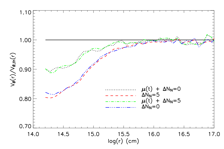
Figures 13a shows the averaged ratio between angular momentum at time t0 and initial angular momentum as a function of particles (ordered in decreasing density) for SPH calculations run with and and the improvement above mentioned either turned on or not. It is clear that time-dependent viscosity better conserve angular momentum for the denser particles. Hence, less angular momentum is transported to the outer part of the core. This is confirmed in Fig. 13b where we plot the ratio between angular momentum at time t0 and initial angular momentum as a function of the radius for the same calculations. Local angular momentum conservation is increased by in the inner part. However, keeping constant the number of neighbors does not improve local angular momentum conservation since the system only evolves over about one free-fall time whereas Attwood et al. (2007) shows that dissipation becomes significant after a few free-fall times. All these improvements of standard SPH are as many new features that will strengthen convergence with the AMR, particle-splitting being the most promising one.
Appendix C Note on the diffusion of the numerical schemes in AMR
A key ingredient in the AMR method is the numerical scheme used to compute flux at the grid’s interfaces. In this paper, we use a Lax-Friedrich (hereafter LF) Riemann solver designed for MHD calculations (Fromang et al. 2006). However, the LF scheme is known to be a diffusive scheme. In this appendix, we present AMR calculations carried out with, on one hand, the LF scheme and, on the other hand, a Roe scheme. Roe scheme being less diffusive than LF, this could have dramatic effect on the fragmentation issue.

C.1 Case ,
Figure 14 shows density maps on the equatorial at three different timesteps for two AMR calculations run with the same numerical parameters, i.e. and , but with a different solver, i.e. the LF one on the left column and the Roe one on the right column. Results are quite similar, AMR calculations are in good agreement for this critical case with the two solvers. Since less angular momentum has been locally lost or transported with the Roe scheme, the core is smaller and the fragments are closer to the central object. This brings support to the fact that we find good convergence between AMR and SPH calculations for this case.
C.2 Case ,
Figure 15 shows density maps on the equatorial plane at t0 + 2 kyr (right column) and t0 + 3 kyr for three simulations of the case , with numerical parameters and (top and bottom maps, LF and Roe schemes) and and (middle row, LF scheme). Let us remind that in Fig. 11, the case and with the LF solver has been displayed. The two calculations with the same numerical parameters differ, according to the numerical scheme used. The fragmentation process changes: one gets a configuration central object + two satellites with the LF scheme whereas we get a binary system resulting from the fragmentation of the central object with the Roe scheme. If we improve the initial sphere resolution in LF calculations (i.e. , ), we converge to the results obtained with the Roe scheme, i.e. a central binary system, with a value . We know that angular momentum is well conserved using the Roe scheme or the LF scheme with , so it seems that calculations lead to a different core fragmentation because of their less accurate angular momentum conservation. Since we use a small thermal support, it is easy to reach another fragmentation configuration, these processes being highly non-linear.

Appendix D Note on SPH sink particles
The introduction of sink particles is a widely used way to get a compromise between good resolution and acceptable timestep in SPH methods. Creating a sink particle enables to loosen the Courant condition on the particle timesteps.
The density level at which a sink particle is created has to be chosen with care. In the previous SPH calculations, no sink particles were used. Let us focus on the highly non-linear fragmentation case, , and to present SPH calculations carried out with various sink densities.
Figure 16 shows calculations carried out with three different densities for the creation of sink particles, , namely g.cm-3 (resulting in no sink creation), g.cm-3 and g.cm-12, from top to bottom, and the same number of SPH particles and neighbors, and . The left-hand side reports results at t0+ 1 kyr and the right-hand column results at t0 + 3 kyr. The CPU time is about 28% smaller for the case g.cm-3 than for the case g.cm-3, but the dense core resulting at t kyr is really different. The upper row corresponds to calculations without creation of sink particles, whereas one sink particle has been created with g.cm-3 and 9 with g.cm-3. It is easy to see that, even if only one sink particle is created, the complete dynamic is affected particularly in the central region.

In conclusion, it is clear that sink particles should be handled with great care. A fair comparison should also compare these SPH calculations with AMR ones including sink particles. Such studies are in progress.