跳到论文正文
W Papers独立论文阅读器 arXiv:0801.3088 论文正文 计算阅读时间 · 0%
引用这篇论文根据当前论文元数据生成,正式投稿前建议核对。


License: arXiv.org perpetual non-exclusive license
arXiv:0801.3088v3 [math.NA] 03 Aug 2008

On Steepest-Descent-Kaczmarz methods for regularizing systems of nonlinear ill-posed equations

A. De Cezaro ††thanks: IMPA, Estr. D. Castorina 110, 22460-320 Rio de Janeiro, Brazil decezaro@impa.br.    M. Haltmeier ††thanks: Department of Computer Science, University of Innsbruck, Technikerstrasse 21a, A-6020 Innsbruck, Austria {markus.haltmeier,otmar.scherzer}@uibk.ac.at.    A. Leitão ††thanks: Department of Mathematics, Federal University of St. Catarina, P.O. Box 476, 88040-900 Florianópolis, Brazil aleitao@mtm.ufsc.br.    O. Scherzer
August 24, 2026
Abstract

We investigate modified steepest descent methods coupled with a loping Kaczmarz strategy for obtaining stable solutions of nonlinear systems of ill-posed operator equations. We show that the proposed method is a convergent regularization method. Numerical tests are presented for a linear problem related to photoacoustic tomography and a non-linear problem related to the testing of semiconductor devices.

Keywords. Nonlinear systems; Ill-posed equations; Regularization; Steepest descent method; Kaczmarz method.

AMS Classification: 65J20, 47J06.

1 Introduction

In this paper we propose a new method for obtaining regularized approximations of systems of nonlinear ill-posed operator equations.

The inverse problem we are interested in consists of determining an unknown physical quantity x∈Xx\in X from the set of data (y0,…,yN−1)∈YN(y_{0},\dots,y_{N-1})\in Y^{N}, where XX, YY are Hilbert spaces and N≥1N\geq 1. In practical situations, we do not know the data exactly. Instead, we have only approximate measured data yiδ∈Yy_{i}^{\delta}\in Y satisfying

∥yiδ−yi∥≤δi,i=0,…,N−1,\|y_{i}^{\delta}-y_{i}\|\leq\delta_{i}\,,\ \ i=0,\dots,N-1\,, (1)

with δi>0\delta_{i}>0 (noise level). We use the notation δ:=(δ0,…,δN−1)\delta:=(\delta_{0},\dots,\delta_{N-1}). The finite set of data above is obtained by indirect measurements of the parameter, this process being described by the model

Fi(x)=yi,i=0,…,N−1,\mathrm{F}_{i}(x)=y_{i}\,,\ \ i=0,\dots,N-1\,, (2)

where Fi:Di⊂X→Y\mathrm{F}_{i}:D_{i}\subset X\to Y, and DiD_{i} are the corresponding domains of definition.

Standard methods for the solution of system (2) are based in the use of Iterative type regularization methods [1, 7, 13, 16, 19] or Tikhonov type regularization methods [7, 23, 30, 32, 33] after rewriting (2) as a single equation F⁡(x)=y\mathrm{F}(x)=y, where

F:=(F0,…,FN−1):⋂i=0N−1Di→YN\displaystyle\mathrm{F}:=(\mathrm{F}_{0},\dots,\mathrm{F}_{N-1}):\bigcap_{i=0}^{N-1}D_{i}\to Y^{N} (3)

and y:=(y0,…,yN−1)y:=(y_{0},\dots,y_{N-1}). However these methods become inefficient if NN is large or the evaluations of Fi​(x)\mathrm{F}_{i}(x) and Fi′​(x)∗\mathrm{F}_{i}^{\prime}(x)^{\ast} are expensive. In such a situation, Kaczmarz type methods [6, 15, 22, 26] which cyclically consider each equation in (2) separately are much faster [24] and are often the method of choice in practice.

For recent analysis of Kaczmarz type methods for systems of ill-posed equations, we refer the reader to [4, 10, 11, 17].

The starting point of our approach is the steepest descent method [7, 29] for solving ill-posed problems. Motivated by the ideas in [10, 11], we propose in this article a loping Steepest-Descent-Kaczmarz method (l-SDK method) for the solution of (2). This iterative method is defined by

xk+1δ=xkδ−ωk​αk​sk,x_{k+1}^{\delta}=x_{k}^{\delta}-\omega_{k}\alpha_{k}s_{k}\,, (4)

where

sk\displaystyle s_{k} :=F[k]′​(xkδ)∗​(F[k]​(xkδ)−y[k]δ),\displaystyle:=\mathrm{F}_{[k]}^{\prime}(x_{k}^{\delta})^{*}(\mathrm{F}_{[k]}(x_{k}^{\delta})-y_{[k]}^{\delta})\,, (5)
ωk\displaystyle\omega_{k} :={1‖F[k]​(xkδ)−y[k]δ‖≥τ​δ[k]0otherwise,\displaystyle:=\begin{cases}1&\|\mathrm{F}_{[k]}(x_{k}^{\delta})-y_{[k]}^{\delta}\|\geq\tau\delta_{[k]}\\ 0&\text{otherwise}\end{cases}\,, (6)
αk\displaystyle\alpha_{k} :={Φrel​(‖sk‖2/‖F[k]′​(xkδ)​sk‖2)ωk=1αminωk=0.\displaystyle:=\begin{cases}\Phi_{\rm rel}\left(\|s_{k}\|^{2}/\|\mathrm{F}_{[k]}^{\prime}(x_{k}^{\delta})s_{k}\|^{2}\right)&\omega_{k}=1\\ \alpha_{\rm min}&\omega_{k}=0\end{cases}\,. (7)

Here αmin>0\alpha_{\rm min}>0, τ∈[2,∞)\tau\in[2,\infty) are appropriate chosen numbers (see (13), (14) below), [k]:=(kmodN)∈{0,…,N−1}[k]:=(k\mod N)\in\{0,\dots,N-1\}, and x0δ=x0∈Xx_{0}^{\delta}=x_{0}\in X is an initial guess, possibly incorporating some a priori knowledge about the exact solution. The function Φrel:(0,∞)→(0,∞)\Phi_{\rm rel}:(0,\infty)\to(0,\infty) defines a sequence of relaxation parameters and is assumed to be continuous, monotonically increasing, bounded by a constant αmax\alpha_{\rm max}, and to satisfy Φ⁡(s)≤s\Phi(s)\leq s (see Figure 1).

Refer to caption
Figure 1: Typical examples for relaxation function Φrel\Phi_{\rm rel}.

If MM is an upper bound for ‖F[k]′​(x)‖\|\mathrm{F}_{[k]}^{\prime}(x)\|, then ‖sk‖2/‖F[k]′​(xkδ)​sk‖2≥1/M2\|s_{k}\|^{2}/\|\mathrm{F}_{[k]}^{\prime}(x_{k}^{\delta})s_{k}\|^{2}\geq 1/M^{2} (cf. Lemma 3.2). Hence the relaxation function Φrel\Phi_{\rm rel} needs only be defined on [1/M2,∞)[1/M^{2},\infty). In particular, if one chooses Φrel​(s)=αmin\Phi_{\rm rel}(s)=\alpha_{\rm min} being constant on that interval, then αk=αmin\alpha_{k}=\alpha_{\rm min} and the l-SDK method reduces to the loping Landweber-Kaczmarz (l-LK) method considered in [10, 11]. The convergence analysis of the l-LK method requires αmin≤1/M2\alpha_{\rm min}\leq 1/M^{2}, whereas the adaptive choice of the relaxation parameters in the present paper allows αk\alpha_{k} being much larger than 1/M21/M^{2}.

The l-SDK method consists in incorporating the Kaczmarz strategy (with the loping parameters ωk\omega_{k}) in the steepest descent method. This strategy is analog to the one introduced in [11] regarding the Landweber-Kaczmarz iteration. As usual in Kaczmarz-type algorithms, a group of NN subsequent steps (starting at some multiple kk of NN) shall be called a cycle. The iteration should be terminated when, for the first time, all xkx_{k} are equal within a cycle. That is, we stop the iteration at

k∗δ:=arg​min⁡{lN∈ℕ:xlNδ=xlN+1δ=⋯=xlN+N−1δ},k_{*}^{\delta}:=\argmin\{lN\in\mathbb{N}:\,x_{lN}^{\delta}=x_{lN+1}^{\delta}=\cdots=x_{lN+N-1}^{\delta}\}\,, (8)

Notice that k∗δk_{*}^{\delta} is the smallest multiple of NN such that

xk∗δ=xk∗δ+1=⋯=xk∗δ+N−1.x_{k_{*}^{\delta}}=x_{k_{*}^{\delta}+1}=\dots=x_{k_{*}^{\delta}+N-1}\,. (9)

In the case of noise free data, δi=0\delta_{i}=0 in (1), we choose ωk≡1\omega_{k}\equiv 1 and the iteration (4) - (7) reduces to the Steepest-Descent-Kaczmarz (SDK) method, which is closely related to the Landweber-Kaczmarz (LK) method considered in [17].

It is worth noticing that, for noisy data, the l-SDK method is fundamentally different from the SDK method: The bang-bang relaxation parameter ωk\omega_{k} effects that the iterates defined in (4) become stationary if all components of the residual vector ‖Fi​(xkδ)−yiδ‖\|\mathrm{F}_{i}(x_{k}^{\delta})-y_{i}^{\delta}\| fall below a pre-specified threshold. This characteristic renders (4) - (7) a regularization method (see Section 3). Another consequence of using these relaxation parameters is the fact that, after a large number of iterations, ωk\omega_{k} will vanish for some kk within each iteration cycle. Therefore, the computational expensive evaluation of F[k]′​(xk)∗\mathrm{F}^{\prime}_{[k]}(x_{k})^{*} might be loped, making the l-SDK method in (4) - (7) a fast alternative to the LK method in [17]. Since in praxis the steepest descent method performs better than the Landweber method, the l-SDK is expected to be more efficient than the l-LK method [10, 11]. Our numerical experiments (mainly for the nonlinear problem considered in Section 5) corroborate this conjecture.

The article is outlined as follows. In Section 2 we formulate basic assumptions and derive some auxiliary estimates required for the analysis. In Section 3 we provide a convergence analysis for the l-SDK method. In Sections 4 and 5 we compare the numerical performance of the l-SDK method with other standard methods for inverse problems in photoacoustic tomography and in semiconductors respectively.

2 Assumptions and Basic Results

We begin this section by introducing some assumptions, that are necessary for the convergence analysis presented in the next section. These assumptions derive from the classical assumptions used in the analysis of iterative regularization methods [7, 16, 29].

First, we assume that the operators Fi\mathrm{F}_{i} are continuously Fréchet differentiable, and also that there exist x0∈Xx_{0}\in X, M>0M>0, and ρ>0\rho>0 such that

‖Fi′​(x)‖≤M,x∈Bρ​(x0)⊂⋂i=0N−1Di.\|\mathrm{F}_{i}^{\prime}(x)\|\leq M\,,\quad\ x\in B_{\rho}(x_{0})\subset\bigcap_{i=0}^{N-1}D_{i}\,. (10)

Notice that x0δ=x0x_{0}^{\delta}=x_{0} is used as starting value of the l-SDK iteration. Next we make an uniform assumption on the nonlinearity of the operators Fi\mathrm{F}_{i}. Namely, we assume that the local tangential cone condition [7, 16]

∥Fi(x)−Fi(x¯)−Fi′(x)(\displaystyle\|\mathrm{F}_{i}(x)-\mathrm{F}_{i}(\bar{x})-\mathrm{F}_{i}^{\prime}(x)( x−x¯)∥Y\displaystyle x-\bar{x})\|_{Y} (11)
≤η​‖Fi​(x)−Fi​(x¯)‖Y,x,x¯∈Bρ​(x0)\displaystyle\leq\eta\|\mathrm{F}_{i}(x)-\mathrm{F}_{i}(\bar{x})\|_{Y}\,,\qquad x,\bar{x}\in B_{\rho}(x_{0})

holds for some η<1/2\eta<1/2. Moreover, we assume the existence of and element

x∗∈Bρ/2​(x0)​ such that ​F​(x∗)=y.x^{*}\in B_{\rho/2}(x_{0})\,\text{ such that }\,\mathrm{F}(x^{*})=y\,. (12)

where y=(y0,…,yN−1)y=(y_{0},\dots,y_{N-1}) are the exact data satisfying (1).

We are now in position to choose the positive constants αmin\alpha_{\rm min}, τ\tau in (7), (6). For the rest of this article we shall assume

αmin:=Φrel​(1/M2),\displaystyle\alpha_{\rm min}:=\Phi_{\rm rel}\left(1/M^{2}\right)\,, (13)
τ≥2​1+η1−2​η≥2.\displaystyle\tau\,\geq 2\,\frac{1+\eta}{1-2\eta}\geq 2\,. (14)

In particular, for linear problems we can choose τ\tau equal to 2.

In the sequel we verify some basic results that are necessary for the convergence analysis derived in the next section. The first result concerns the well-definedness and positivity of the relaxation parameter αk\alpha_{k}.

Lemma 2.1.

Let assumptions (10) - (12) be satisfied. Then the coefficients αk\alpha_{k} in (7) are well-defined and positive.

Proof.

If ωk=0\omega_{k}=0, the assertion follows from (7). If ωk=1\omega_{k}=1, then ‖F[k]​(xkδ)−y[k]δ‖≥τ​δ[k]\|\mathrm{F}_{[k]}(x_{k}^{\delta})-y_{[k]}^{\delta}\|\geq\tau\delta_{[k]} and the assertion is a consequence of [29, Lemma 3.1], applied to F[k]\mathrm{F}_{[k]} instead of F\mathrm{F}. ∎

In the next lemma we prove an estimate for the step size of the l-SDK iteration.

Lemma 2.2.

Let sks_{k} and αk\alpha_{k} be defined by (5) and (7). Then

αk​‖sk‖2≤‖F[k]​(xkδ)−y[k]δ‖2,k∈ℕ.\alpha_{k}\|s_{k}\|^{2}\ \leq\ \|\mathrm{F}_{[k]}(x_{k}^{\delta})-y_{[k]}^{\delta}\|^{2}\,,\qquad k\in\mathbb{N}\,. (15)
Proof.

It is enough to consider the case ωk=1\omega_{k}=1. It follows from (7) that

αk​‖sk‖2=Φrel​(‖sk‖2‖F[k]′​(xkδ)​sk‖2)​‖sk‖2≤‖sk‖4‖F[k]′​(xkδ)​sk‖2.\alpha_{k}\|s_{k}\|^{2}\ =\ \Phi_{\rm rel}\left(\frac{\|s_{k}\|^{2}}{\|\mathrm{F}_{[k]}^{\prime}(x_{k}^{\delta})\,s_{k}\|^{2}}\right)\|s_{k}\|^{2}\ \leq\ \frac{\|s_{k}\|^{4}}{\|\mathrm{F}_{[k]}^{\prime}(x_{k}^{\delta})\,s_{k}\|^{2}}\,. (16)

Moreover, from the definition of sks_{k} we obtain

‖F[k]′​(xkδ)​sk‖=‖F[k]′​(xkδ)​F[k]′​(xkδ)∗​[F[k]​(xkδ)−y[k]δ]‖,\displaystyle\|\mathrm{F}_{[k]}^{\prime}(x_{k}^{\delta})\,s_{k}\|\ =\ \|\mathrm{F}_{[k]}^{\prime}(x_{k}^{\delta})\mathrm{F}_{[k]}^{\prime}(x_{k}^{\delta})^{*}[\mathrm{F}_{[k]}(x_{k}^{\delta})-y_{[k]}^{\delta}]\|\,,
‖sk‖2≤‖F[k]′​(xkδ)​F[k]′​(xkδ)∗​[F[k]​(xkδ)−y[k]δ]‖​‖F[k]​(xkδ)−y[k]δ‖.\displaystyle\|s_{k}\|^{2}\ \leq\ \|\mathrm{F}_{[k]}^{\prime}(x_{k}^{\delta})\mathrm{F}_{[k]}^{\prime}(x_{k}^{\delta})^{*}[\mathrm{F}_{[k]}(x_{k}^{\delta})-y_{[k]}^{\delta}]\|\,\|\mathrm{F}_{[k]}(x_{k}^{\delta})-y_{[k]}^{\delta}\|\,.

Now, substituting the last two expressions in (16), shows (15). ∎

The following Lemma is an important auxiliary result, which will be used at several places throughout this article.

Lemma 2.3.

Let xkδx_{k}^{\delta}, αk\alpha_{k}, ωk\omega_{k}, and sks_{k} be defined by (4) - (7) and assume that (10) - (12) hold true. If xkδ∈Bρ/2​(x∗)x_{k}^{\delta}\in B_{\rho/2}(x^{*}) for some k≥0k\geq 0, then

∥\displaystyle\| xk+1δ−x∗∥2−∥xkδ−x∗∥2\displaystyle x_{k+1}^{\delta}-x^{*}\|^{2}-\|x_{k}^{\delta}-x^{*}\|^{2} (17)
≤ωk​αk​‖F[k]​(xkδ)−y[k]δ‖​((2​η−1)​‖F[k]​(xkδ)−y[k]δ‖+2​(1+η)​δ[k]).\displaystyle\leq\omega_{k}\alpha_{k}\|\mathrm{F}_{[k]}(x_{k}^{\delta})-y_{[k]}^{\delta}\|\Big((2\eta-1)\|\mathrm{F}_{[k]}(x_{k}^{\delta})-y_{[k]}^{\delta}\|+2(1+\eta)\delta_{[k]}\Big)\,.\quad{}
Proof.

If ωk=0\omega_{k}=0, then xk+1=xkx_{k+1}=x_{k} and (17) follows with equality. If ωk=1\omega_{k}=1, it follows from (4) and (5) and Lemma 2.2 that

‖xk+1δ−x∗‖2−‖xkδ−x∗‖2\displaystyle\|x_{k+1}^{\delta}-x^{*}\|^{2}-\|x_{k}^{\delta}-x^{*}\|^{2}
=2​⟨xkδ−x∗,xk+1δ−xkδ⟩+‖xk+1δ−xkδ‖2\displaystyle\quad=2\langle x_{k}^{\delta}-x^{*},\ x_{k+1}^{\delta}-x_{k}^{\delta}\rangle+\|x_{k+1}^{\delta}-x_{k}^{\delta}\|^{2}
=2​αk​⟨xkδ−x∗,F[k]′​(xkδ)∗​(y[k]δ−F[k]​(xkδ))⟩+αk2​‖sk‖2\displaystyle\quad=2\alpha_{k}\langle x_{k}^{\delta}-x^{*},\ \mathrm{F}^{\prime}_{[k]}(x_{k}^{\delta})^{*}(y_{[k]}^{\delta}-\mathrm{F}_{[k]}(x_{k}^{\delta}))\rangle+\alpha_{k}^{2}\|s_{k}\|^{2}
≤2​k​αk​⟨y[k]δ−F[k]​(xkδ),F[k]′​(xkδ)​(xkδ−x∗)⟩+αk​‖F[k]​(xkδ)−y[k]δ‖2\displaystyle\quad\leq 2k\alpha_{k}\langle y_{[k]}^{\delta}-\mathrm{F}_{[k]}(x_{k}^{\delta}),\mathrm{F}^{\prime}_{[k]}(x_{k}^{\delta})(x_{k}^{\delta}-x^{*})\rangle+\alpha_{k}\|\mathrm{F}_{[k]}(x_{k}^{\delta})-y_{[k]}^{\delta}\|^{2}
≤αk​(2​⟨y[k]δ−F[k]​(xkδ),F[k]′​(xkδ)​(xkδ−x∗)−F[k]​(x∗)+F[k]​(xkδ)⟩CLOSE\displaystyle\quad\leq\alpha_{k}\Bigl(2\langle y_{[k]}^{\delta}-\mathrm{F}_{[k]}(x_{k}^{\delta}),\ \mathrm{F}^{\prime}_{[k]}(x_{k}^{\delta})(x_{k}^{\delta}-x^{*})-\mathrm{F}_{[k]}(x^{*})+\mathrm{F}_{[k]}(x_{k}^{\delta})\rangle
OPEN+2​⟨y[k]δ−F[k]​(xkδ),y[k]−y[k]δ⟩−‖y[k]δ−F[k]​(xkδ)‖2).\displaystyle\qquad\qquad\qquad+2\langle y_{[k]}^{\delta}-\mathrm{F}_{[k]}(x_{k}^{\delta}),\ y_{[k]}-y_{[k]}^{\delta}\rangle-\|y_{[k]}^{\delta}-\mathrm{F}_{[k]}(x_{k}^{\delta})\|^{2}\;\Bigr)\,.

Now, applying (11) with x=x∗x=x^{*} and x¯=xkδ∈Bρ/2​(x∗)⊂Bρ​(x0)\bar{x}=x_{k}^{\delta}\in B_{\rho/2}(x^{*})\subset B_{\rho}(x_{0}), leads to

‖xk+1δ−x∗‖2−‖xkδ−x∗‖2\displaystyle\|x_{k+1}^{\delta}-x^{*}\|^{2}-\|x_{k}^{\delta}-x^{*}\|^{2}
≤ωk​αk​‖F[k]​(xkδ)−y[k]δ‖​(2​η​‖F[k]​(xkδ)−y[k]‖+2​δ[k]−‖F[k]​(xkδ)−y[k]δ‖).\displaystyle\quad\leq\omega_{k}\alpha_{k}\|\mathrm{F}_{[k]}(x_{k}^{\delta})-y_{[k]}^{\delta}\|\,\Big(2\eta\|\mathrm{F}_{[k]}(x_{k}^{\delta})-y_{[k]}\|+2\delta_{[k]}-\|\mathrm{F}_{[k]}(x_{k}^{\delta})-y_{[k]}^{\delta}\|\,\Big)\,.

The last inequality and (1) show (17).∎

Our next goal is to prove a monotony property, known to be satisfied by other iterative regularization methods, e.g., by the Landweber [7], the steepest descent [29], the LK [17], and the l-LK [11] method.

Proposition 2.4 (Monotonicity).

Under the assumptions of Lemma 2.3,

‖xk+1δ−x∗‖2\displaystyle\|x_{k+1}^{\delta}-x^{*}\|^{2} ≤‖xkδ−x∗‖2,k∈ℕ.\displaystyle\leq\|x_{k}^{\delta}-x^{*}\|^{2}\,,\ \qquad k\in\mathbb{N}\,. (18)

Moreover, all iterates xkδx_{k}^{\delta} remain in Bρ/2​(x∗)⊂Bρ​(x0)B_{\rho/2}(x^{*})\subset B_{\rho}(x_{0}) and satisfy (17).

Proof.

From (12) it follows that x0∈Bρ/2​(x∗)x_{0}\in B_{\rho/2}(x^{*}). If ωδ=0\omega^{\delta}=0, then x1x_{1} satisfies (18) with equality and x1∈Bρ/2​(x∗)⊂Bρ​(x0)x_{1}\in B_{\rho/2}(x^{*})\subset B_{\rho}(x_{0}). If ωδ≠0\omega^{\delta}\not=0, then Lemma 2.3 implies

‖x1δ−x∗‖2−‖x0δ−x∗‖2\displaystyle\|x_{1}^{\delta}-x^{*}\|^{2}-\|x_{0}^{\delta}-x^{*}\|^{2} ≥(2​η−1)​‖F0​(x0δ)−yδ,0‖+2​(1+η)​δ0\displaystyle\geq(2\eta-1)\|\mathrm{F}_{0}(x_{0}^{\delta})-y^{\delta,0}\|+2(1+\eta)\delta^{0}
≥δ0​((2​η−1)​τ+2​(1+η))≥0.\displaystyle\geq\delta_{0}\Big((2\eta-1)\tau+2(1+\eta)\Big)\geq 0\,.

Therefore (18), for k=0k=0, follows from (14). In particular, x1∈Bρ/2​(x∗)x_{1}\in B_{\rho/2}(x^{*}). An inductive argument implies (18) and that xk∈Bρ/2​(x∗)⊂Bρ​(x0)x_{k}\in B_{\rho/2}(x^{*})\subset B_{\rho}(x_{0}) for all k∈ℕk\in\mathbb{N}. The assertions therefore follows from Lemma 2.3. ∎

3 Convergence Analysis of the Loping Steepest Descent Kaczmarz Method

In this section we provide a complete convergence analysis for the l-SDK iteration, showing that it is a convergent regularization method in the sense of [7] (see Theorems 3.3 and 3.6 below). Throughout this section, we assume that (10) - (14) hold, and that xkδx_{k}^{\delta}, αk\alpha_{k}, ωk\omega_{k}, and sks_{k} are defined by (4) - (7).

Our first goal is to prove convergence of the l-SDK iteration for δ=0\delta=0. For exact data y=(y0,…,yN−1)y=(y_{0},\dots,y_{N-1}), the iterates in (4) are denoted by xkx_{k}.22 2 This is a standard notation used in the literature.

Lemma 3.1.

There exists an x0x_{0}-minimal norm solution of (2) in Bρ/2​(x0)B_{\rho/2}(x_{0}), i.e., a solution x†x^{\dagger} of (2) such that

‖x†−x0‖=inf{‖x−x0‖:x∈Bρ/2​(x0)​ and ​F​(x)=y}.\displaystyle\|x^{\dagger}-x_{0}\|=\inf\big\{\|x-x_{0}\|:x\in B_{\rho/2}(x_{0})\text{ and }\mathrm{F}(x)=y\}\,.

Moreover, x†x^{\dagger} is the only solution of (2) in Bρ/2​(x0)∩(x0+ker⁡(F′​(x†))⟂)B_{\rho/2}(x_{0})\cap\bigl(x_{0}+\ker(\mathrm{F}^{\prime}(x^{\dagger}))^{\perp}\bigr).

Proof.

Lemma 3.1 is a consequence of [13, Proposition 2.1]. A detailed proof can be found in [16]. ∎

Lemma 3.2.

For all k∈ℕk\in\mathbb{N}, we have αk≥αmin\alpha_{k}\geq\alpha_{\rm min}.

Proof.

For ωk=0\omega_{k}=0 the claimed estimate holds with equality. If ωk=1\omega_{k}=1, it follows from (10) that

‖sk‖2/‖F[k]′​(xkδ)​sk‖2≥‖F[k]′​(xkδ)‖−2≥ 1/M2.\displaystyle\|s_{k}\|^{2}/\|\mathrm{F}_{[k]}^{\prime}(x_{k}^{\delta})\,s_{k}\|^{2}\ \geq\ \|\mathrm{F}_{[k]}^{\prime}(x_{k}^{\delta})\|^{-2}\ \geq\ 1/M^{2}\,.

Now the monotonicity of Φrel\Phi_{\rm rel} implies αk≥Φrel​(M−2)=αmin\alpha_{k}\geq\Phi_{\rm rel}(M^{-2})=\alpha_{\rm min}. ∎

Throughout the rest of this article, x†x^{\dagger} denotes the x0x_{0}-minimal norm solution of (2). We define ek:=x†−xke_{k}:=x^{\dagger}-x_{k}. From Proposition 2.4 it follows that (17) holds for all kk. By summing over all kk, this leads to

∑i=0∞αi​‖y[i]−F[i]​(xi)‖2≤‖x0−x†‖21−2​η<∞.\displaystyle\sum_{i=0}^{\infty}\alpha_{i}\|y_{[i]}-\mathrm{F}_{[i]}(x_{i})\|^{2}\ \leq\ \frac{\|x_{0}-x^{\dagger}\|^{2}}{1-2\eta}\ <\ \infty\,. (19)

Equation (19) and the monotony of ‖ek‖\|e_{k}\| shown in Proposition 2.4 are main ingredients in the following proof of the convergence of the SDK iteration.

Theorem 3.3 (Convergence for Exact Data).

For exact data, the iteration (xk)(x_{k}) converges to a solution of (2), as k→∞k\to\infty. Moreover, if

𝒩⁡(F′​(x†))⊆𝒩⁡(F′​(x)) for all ​x∈Bρ​(x0),\nr(\mathrm{F}^{\prime}(x^{\dagger}))\subseteq\nr(\mathrm{F}^{\prime}(x))\quad\text{ for all }x\in B_{\rho}(x_{0})\,, (20)

then xk→x†x_{k}\to x^{\dagger}.

Proof.

From (18) it follows that ‖ek‖\|e_{k}\| decreases monotonically and therefore that ‖ek‖\|e_{k}\| converges to some ϵ≥0\epsilon\geq 0. In the following we show that eke_{k} is in fact a Cauchy sequence.

For k=k0​N+k1k=k_{0}N+k_{1} and l=l0​N+l1l=l_{0}N+l_{1} with k≤lk\leq l and k1,l1∈{0,…,N−1}k_{1},l_{1}\in\{0,\dots,N-1\}, let n0∈{k0,…,l0}n_{0}\in\{k_{0},\dots,l_{0}\} be such that

∑i1=0N−1‖Fi1​(xN​n0+i1)−yi1‖≤∑i1=0N−1‖Fi1​(xN​i0+i1)−yi1‖,i0∈{k0,…,l0}.\sum_{i_{1}=0}^{N-1}\|F_{i_{1}}(x_{Nn_{0}+i_{1}})-y_{i_{1}}\|\leq\sum_{i_{1}=0}^{N-1}\|F_{i_{1}}(x_{Ni_{0}+i_{1}})-y_{i_{1}}\|\,,\quad i_{0}\in\{k_{0},\dots,l_{0}\}\,. (21)

Then, with n:=N​n0+N−1n:=Nn_{0}+N-1, we have

‖ek−el‖≤‖ek−en‖+‖el−en‖\|e_{k}-e_{l}\|\leq\|e_{k}-e_{n}\|+\|e_{l}-e_{n}\| (22)

and

‖en−ek‖2\displaystyle\|e_{n}-e_{k}\|^{2} =‖ek‖2−‖en‖2+2​⟨en−ek,en⟩.\displaystyle=\|e_{k}\|^{2}-\|e_{n}\|^{2}+2\langle e_{n}-e_{k},e_{n}\rangle\,. (23)
‖en−el‖2\displaystyle\|e_{n}-e_{l}\|^{2} =‖el‖2−‖en‖2+2​⟨en−el,en⟩,\displaystyle=\|e_{l}\|^{2}-\|e_{n}\|^{2}+2\langle e_{n}-e_{l},e_{n}\rangle\,,

For k→∞k\to\infty, the first two terms of (23) converge to ϵ−ϵ=0\epsilon-\epsilon=0. Therefore, in order to show that eke_{k} is a Cauchy sequence, it is sufficient to prove that ⟨en−ek,en⟩\langle e_{n}-e_{k},e_{n}\rangle and ⟨en−el,en⟩\langle e_{n}-e_{l},e_{n}\rangle converge to zero as k→∞k\to\infty.

To that end, we write i=N​i0+i1i=Ni_{0}+i_{1}, i1∈{0,…,N−1}i_{1}\in\{0,\dots,N-1\} and set i∗:=N​n0+i1i^{*}:=Nn_{0}+i_{1}. Then, using the definition of the steepest descent Kaczmarz iteration it follows that

|⟨\displaystyle|\langle en−ek,en⟩|\displaystyle e_{n}-e_{k},e_{n}\rangle|
=|∑i=kn−1αi​⟨Fi1′​(xi)∗​(yi1−Fi1​(xi)),x†−xn⟩|\displaystyle=\biggl|\sum_{i=k}^{n-1}\alpha_{i}\big\langle\mathrm{F}_{i_{1}}^{\prime}(x_{i})^{*}\big(y_{i_{1}}-\mathrm{F}_{i_{1}}(x_{i})\big),x^{\dagger}-x_{n}\big\rangle\biggr|
≤∑i=kn−1αi​|⟨yi1−Fi1​(xi),Fi1′​(xi)​(x†−xi∗)+Fi1′​(xi)​(xi∗−xn)⟩|\displaystyle\leq\sum_{i=k}^{n-1}\alpha_{i}\left|\big\langle y_{i_{1}}-\mathrm{F}_{i_{1}}(x_{i}),\mathrm{F}_{i_{1}}^{\prime}(x_{i})(x^{\dagger}-x_{i^{*}})+\mathrm{F}_{i_{1}}^{\prime}(x_{i})(x_{i^{*}}-x_{n})\big\rangle\right|
≤∑i=kn−1αi​‖yi1−Fi1​(xi)‖​‖Fi1′​(xi)​(x†−xi∗)‖\displaystyle\leq\sum_{i=k}^{n-1}\alpha_{i}\|y_{i_{1}}-\mathrm{F}_{i_{1}}(x_{i})\|\,\|\mathrm{F}_{i_{1}}^{\prime}(x_{i})(x^{\dagger}-x_{i^{*}})\|
+∑i=kn−1αi∥yi1−Fi1(xi)∥∥Fi1′(xi)(xi∗−xn)∥\displaystyle\qquad\qquad\;+\sum_{i=k}^{n-1}\alpha_{i}\|y_{i_{1}}-\mathrm{F}_{i_{1}}(x_{i})\|\,\|\mathrm{F}_{i_{1}}^{\prime}(x_{i})(x_{i^{*}}-x_{n})\| (24)

From (11) it follows that

‖Fi1′​(xi)​(x†−xi∗)‖≤2​(1+η)​‖yi1−Fi1​(xi)‖+(1+η)​‖yi1−Fi1​(xi∗)‖.\displaystyle\|\mathrm{F}_{i_{1}}^{\prime}(x_{i})(x^{\dagger}-x_{i^{*}})\|\leq 2(1+\eta)\|y_{i_{1}}-\mathrm{F}_{i_{1}}(x_{i})\|+(1+\eta)\|y_{i_{1}}-\mathrm{F}_{i_{1}}(x_{i^{*}})\|\,. (25)

Again using the definition of the steepest descent Kaczmarz iteration and equations (7), (10), it follows that

∥Fi1′(xi)(xi∗−\displaystyle\|\mathrm{F}_{i_{1}}^{\prime}(x_{i})(x_{i^{*}}- OPENxn)|≤M​‖xi∗−xn‖\displaystyle x_{n})\|\leq M\,\|x_{i^{*}}-x_{n}\|
≤M​∑j=i1N−2αj​‖Fj′​(xN​n0+j)∗​(Fj​(xN​n0+j)−yj)‖\displaystyle\leq M\,\sum_{j=i_{1}}^{N-2}\alpha_{j}\|\mathrm{F}_{j}^{\prime}(x_{Nn_{0}+j})^{*}\big(\mathrm{F}_{j}(x_{Nn_{0}+j})-y_{j}\big)\|
≤αmax​M2​∑j=0N−1‖Fj​(xN​n0+j)−yj‖.\displaystyle\leq\alpha_{\rm max}M^{2}\sum_{j=0}^{N-1}\|F_{j}(x_{Nn_{0}+j})-y_{j}\|\,. (26)

Substituting (25), (26) in (24) leads to

|⟨\displaystyle|\langle en−ek,en⟩|\displaystyle e_{n}-e_{k},e_{n}\rangle|
≤c​∑i0=k0n−1∑i1=0N−1‖yi1−Fi1​(xN​i0+i1)‖​(∑j=0N−1‖Fj​(xN​n0+j)−yj‖)\displaystyle\leq c\sum_{i_{0}=k_{0}}^{n-1}\sum_{i_{1}=0}^{N-1}\|y_{i_{1}}-\mathrm{F}_{i_{1}}(x_{Ni_{0}+i_{1}})\|\left(\sum_{j=0}^{N-1}\|\mathrm{F}_{j}(x_{Nn_{0}+j})-y_{j}\|\right)
≤c​∑i0=k0n−1(∑i1=0N−1‖yi1−Fi1​(xN​i0+i1)‖)2\displaystyle\leq c\sum_{i_{0}=k_{0}}^{n-1}\Bigl(\sum_{i_{1}=0}^{N-1}\|y_{i_{1}}-\mathrm{F}_{i_{1}}(x_{Ni_{0}+i_{1}})\|\Bigr)^{2}

with c:=αmax​(3+3​η+αmax​M2)c:=\alpha_{\rm max}(3+3\eta+\alpha_{\rm max}M^{2}). Here we made use of (21). So, we finally obtain the estimate

|⟨\displaystyle|\langle en−ek,en⟩|≤N​cαmin∑i0=k0n−1∑i1=0N−1αN​i0+i1∥yi1−Fi1(xN​i0+i1)∥2.\displaystyle e_{n}-e_{k},e_{n}\rangle|\leq\frac{Nc}{\alpha_{\rm min}}\sum_{i_{0}=k_{0}}^{n-1}\sum_{i_{1}=0}^{N-1}\alpha_{Ni_{0}+i_{1}}\|y_{i_{1}}-\mathrm{F}_{i_{1}}(x_{Ni_{0}+i_{1}})\|^{2}\,.

Because of (19), the last sum tends to zero for k=N​k0+k1→∞k=Nk_{0}+k_{1}\to\infty, and therefore ⟨en,en−ek⟩→0\langle e_{n},e_{n}-e_{k}\rangle\to 0. Analogously one shows that ⟨en,en−el⟩→0\langle e_{n},e_{n}-e_{l}\rangle\to 0. Therefore eke_{k} is a Cauchy sequence and xk=x†−ekx_{k}=x^{\dagger}-e_{k} converges to an element x∗∈Xx^{\ast}\in X. Because all residuals ‖F[k]​(xk)−y[k]‖\|\mathrm{F}_{[k]}(x_{k})-y_{[k]}\| tend to zero, x∗x^{*} is solution of (2).

Now assume 𝒩⁡(F′​(x†))⊆𝒩⁡(F⁡(x))\nr(\mathrm{F}^{\prime}(x^{\dagger}))\subseteq\nr(\mathrm{F}(x)), for x∈Bρ​(x0)x\in B_{\rho}(x_{0}). Then from the definition of xkx_{k} it follows that

xk+1−xk∈ℛ⁡(F[k]′​(xk)∗)⊂𝒩⁡(F[k]′​(xk))⊥⊂𝒩⁡(F′​(xk))⊥⊂𝒩⁡(F′​(x†))⊥.\displaystyle x_{k+1}-x_{k}\in\ra(\mathrm{F}_{[k]}^{\prime}(x_{k})^{*})\subset\nr(\mathrm{F}_{[k]}^{\prime}(x_{k}))^{\bot}\subset\nr(\mathrm{F}^{\prime}(x_{k}))^{\bot}\subset\nr(\mathrm{F}^{\prime}(x^{\dagger}))^{\bot}\,.

An inductive argument shows that all iterates xkx_{k} are elements of x0+𝒩⁡(F′​(x†))⊥x_{0}+\nr(\mathrm{F}^{\prime}(x^{\dagger}))^{\bot}. Together with the continuity of F′​(x†)\mathrm{F}^{\prime}(x^{\dagger}) this implies that x∗∈x0+𝒩⁡(F′​(x†))⊥x^{*}\in x_{0}+\nr(\mathrm{F}^{\prime}(x^{\dagger}))^{\bot}. By Lemma 3.1, x†x^{\dagger} is the only solution of (2) in Bρ/2​(x0)∩(x0+𝒩⁡(F′​(x†))⟂)B_{\rho/2}(x_{0})\cap\bigl(x_{0}+\nr(\mathrm{F}^{\prime}(x^{\dagger}))^{\perp}\bigr), and so the second assertion follows. ∎

The second goal in this section is to prove that xk∗δx_{k*}^{\delta} converges to a solution of (2), as δ→0\delta\to 0. First we verify that, for noisy data, the stopping index k∗δk_{*}^{\delta} defined in (8) is finite.

Proposition 3.4 (Stopping Index).

Assume δmin:=min⁡{δ0,…,δN−1}>0\delta_{\rm min}:=\min\{\delta_{0},\dots,\delta_{N-1}\}>0. Then k∗δk_{*}^{\delta} defined in (8) is finite, and

∥Fi(xk∗δδ)−yiδ∥<τδi,i=0,…,N−1.\|\mathrm{F}_{i}(x_{k_{*}^{\delta}}^{\delta})-y_{i}^{\delta}\|<\tau\delta_{i}\,,\qquad i=0,\dots,N-1\,. (27)
Proof.

Assume that for every l∈Nl\in N, there exists i⁡(l)∈{0,…,N−1}i(l)\in\{0,\dots,N-1\} such that xl​N+i⁡(l)≠xl​Nx_{lN+i(l)}\not=x_{lN}. From Proposition 2.4 follows that we can apply (17) recursively for k=1,…,l​Nk=1,\dots,lN and obtain

−‖x0−x∗‖2≤\displaystyle-\|x_{0}-x^{*}\|^{2}\leq ∑k=1l​Nωk​αk​‖F[k]​(xkδ)−y[k]δ‖\displaystyle\sum_{k=1}^{lN}\omega_{k}\alpha_{k}\|\mathrm{F}_{[k]}(x_{k}^{\delta})-y_{[k]}^{\delta}\|
(2​(1+η)​δ[k]−(1−2​η)​‖F[k]​(xkδ)−y[k]δ‖),l∈ℕ.\displaystyle\left(2(1+\eta)\delta_{[k]}-(1-2\eta)\|\mathrm{F}_{[k]}(x_{k}^{\delta})-y_{[k]}^{\delta}\|\right)\,,\quad l\in\mathbb{N}\,.

Using the fact that either ωk=0\omega_{k}=0 or ‖F[k]​(xkδ)−y[k]δ‖≥τ​δ[k]\|\mathrm{F}_{[k]}(x_{k}^{\delta})-y_{[k]}^{\delta}\|\geq\tau\delta_{[k]}, we obtain

‖x0−x∗‖2≥(τ⁡(1−2​η)−2​(1+η))​∑k=1l​Nωk​αk​δ[k]​‖F[k]​(xkδ)−y[k]δ‖.\|x_{0}-x^{*}\|^{2}\geq\Bigl(\tau(1-2\eta)-2(1+\eta)\Bigr)\sum_{k=1}^{lN}\,\omega_{k}\alpha_{k}\delta_{[k]}\|\mathrm{F}_{[k]}(x_{k}^{\delta})-y_{[k]}^{\delta}\|\,. (28)

Equation (28), Lemma 3.2 and the fact that xl′​N+i⁡(l′)≠xl′​Nx_{l^{\prime}N+i(l^{\prime})}\not=x_{l^{\prime}N} for all l′∈ℕl^{\prime}\in\mathbb{N}, imply

‖x0−x∗‖2≥(τ⁡(1−2​η)−2​(1+η))​l​αmin​δmin​(τ​δmin),l∈ℕ.\|x_{0}-x^{*}\|^{2}\ \geq\ \Bigl(\tau(1-2\eta)-2(1+\eta)\Bigr)\,l\,\alpha_{\rm min}\,\delta_{\rm min}\,(\tau\delta_{\rm min})\,,\quad l\in\mathbb{N}\,. (29)

The right hand side of (29) tends to infinity, which gives a contradiction. Consequently, {l∈ℕ:xl​N+i=xl​N, 0≤i≤N−1}≠∅\{l\in\mathbb{N}:x_{lN+i}=x_{lN}\,,\,0\leq i\leq N-1\}\not=\emptyset and the infimum in (8) takes a finite value.

To prove (27), assume to the contrary, that ‖Fi​(xk∗δδ)−yiδ‖≥τ​δi\|\mathrm{F}_{i}(x_{k_{*}^{\delta}}^{\delta})-y_{i}^{\delta}\|\geq\tau\delta_{i} for some i∈{0,…,N−1}i\in\{0,\dots,N-1\}. From (6) and (8) it follows that, ωk∗δ=1\omega_{k_{*}^{\delta}}=1 and xk∗δ+iδ=xk∗δ+i+1δx_{k_{*}^{\delta}+i}^{\delta}=x_{k_{*}^{\delta}+i+1}^{\delta} respectively. Thus, Proposition 2.4 and Lemma 2.1 imply

0≤(2​η−1)​‖Fi​(xk∗δδ)−yiδ‖+2​(1+η)​δi<δi​((2​η−1)​τ+2​(1+η)).\displaystyle 0\leq(2\eta-1)\|\mathrm{F}_{i}(x_{k_{*}^{\delta}}^{\delta})-y_{i}^{\delta}\|+2(1+\eta)\delta_{i}<\delta_{i}\Big((2\eta-1)\tau+2(1+\eta)\Big)\,.

This contradicts (14), concluding the proof of (27). ∎

The last auxiliary result concerns the continuity of xkδx_{k}^{\delta} at δ=0\delta=0. For y,yδ∈YNy,y^{\delta}\in Y^{N}, δ>0\delta>0, and k∈ℕk\in\mathbb{N} we define

Δk​(δ,y,yδ)\displaystyle\Delta_{k}(\delta,y,y^{\delta}) :=ωk​F[k]′​(xkδ)∗​(F[k]​(xkδ)−y[k]δ)−F[k]′​(xk)∗​(F[k]​(xk)−y[k]).\displaystyle:=\omega_{k}\mathrm{F}_{[k]}^{\prime}(x_{k}^{\delta})^{*}\bigl(\mathrm{F}_{[k]}(x_{k}^{\delta})-y_{[k]}^{\delta}\bigr)-\mathrm{F}_{[k]}^{\prime}(x_{k})^{*}\bigl(\mathrm{F}_{[k]}(x_{k})-y_{[k]}\bigr)\,.
Lemma 3.5.

For all k∈ℕk\in\mathbb{N},

limδ→0sup{∥Δk(δ,y,yδ)∥:yδ∈YN,∥yi−yiδ∥≤δi}=0.\displaystyle\lim_{\delta\to 0}\sup\left\{\|\Delta_{k}(\delta,y,y^{\delta})\|:y^{\delta}\in Y^{N},\,\|y_{i}-y_{i}^{\delta}\|\leq\delta_{i}\right\}=0\;. (30)

Moreover, xk+1δ→xk+1x_{k+1}^{\delta}\to x_{k+1}, as δ→0\delta\to 0.

Proof.

We prove Lemma 3.5 by induction. The case k=0k=0 is similar to the general case and is omitted.

Now, assume k>0k>0 and that (30) holds for all k′<kk^{\prime}<k. First we note that (30) and the continuity of Φrel\Phi_{\rm rel} obviously imply xk+1δ→xk+1x_{k+1}^{\delta}\to x_{k+1}, as δ→0\delta\to 0. For the proof of (30) we consider two cases. In the first case, ωk=1\omega_{k}=1, we have

‖Δk​(δ,y,yδ)‖\displaystyle\|\Delta_{k}(\delta,y,y^{\delta})\| =‖F[k]′​(xkδ)∗​(F[k]​(xkδ)−y[k]δ)−F[k]′​(xk)∗​(F[k]​(xk)−y[k])‖.\displaystyle=\|\mathrm{F}_{[k]}^{\prime}(x_{k}^{\delta})^{*}\bigl(\mathrm{F}_{[k]}(x_{k}^{\delta})-y_{[k]}^{\delta}\bigr)-\mathrm{F}_{[k]}^{\prime}(x_{k})^{*}\bigl(\mathrm{F}_{[k]}(x_{k})-y_{[k]}\bigr)\|\,.

In the second case, ωk=0\omega_{k}=0, we have ‖F[k]​(xkδ)−y[k]δ‖≤τ​δk\|\mathrm{F}_{[k]}(x_{k}^{\delta})-y_{[k]}^{\delta}\|\leq\tau\delta^{k} and consequently

∥Δk\displaystyle\|\Delta_{k} (δ,y,yδ)|≤‖F[k]′​(xk)∗​(F[k]​(xk)−y[k])‖\displaystyle(\delta,y,y^{\delta})\|\leq\|\mathrm{F}_{[k]}^{\prime}(x_{k})^{*}(\mathrm{F}_{[k]}(x_{k})-y_{[k]})\|
≤‖F[k]′​(xkδ)‖​(‖F[k]​(xk)−F[k]​(xkδ)‖+‖F[k]​(xkδ)−ykδ‖+‖ykδ−y[k]‖)\displaystyle\leq\|\mathrm{F}_{[k]}^{\prime}(x_{k}^{\delta})\|\left(\|\mathrm{F}_{[k]}(x_{k})-\mathrm{F}_{[k]}(x_{k}^{\delta})\|+\|\mathrm{F}_{[k]}(x_{k}^{\delta})-y_{k}^{\delta}\|+\|y_{k}^{\delta}-y_{[k]}\|\right)
≤‖F[k]′​(xkδ)‖​(‖F[k]​(xk)−F[k]​(xkδ)‖+(τ+1)​δ[k]).\displaystyle\leq\|\mathrm{F}_{[k]}^{\prime}(x_{k}^{\delta})\|\left(\|\mathrm{F}_{[k]}(x_{k})-\mathrm{F}_{[k]}(x_{k}^{\delta})\|+(\tau+1)\,\delta_{[k]}\right)\,.

Now (30) follows from (10), the continuity of F[k]F_{[k]} and F[k]′F^{\prime}_{[k]}, and the induction hypothesis (which implies xkδ→xkx_{k}^{\delta}\to x_{k}). ∎

Theorem 3.6 (Convergence for Noisy Data).

Assume (δ0j,…,δN−1j)(\delta^{j}_{0},\dots,\delta^{j}_{N-1}) is a sequence in (0,∞)N(0,\infty)^{N} with limj→∞δij=0\lim_{j\to\infty}\delta^{j}_{i}=0. Let (y0j,…,yN−1j)(y^{j}_{0},\dots,y^{j}_{N-1}) be a sequence of noisy data satisfying

∥yij−yi∥≤δji,i=0,…,N−1,j∈ℕ,\displaystyle\|y_{i}^{j}-y_{i}\|\leq\delta^{j}_{i}\,,\qquad i=0,\dots,N-1\,,\,j\in\mathbb{N}\,,

and let kj:=k∗​(δj,yj)k^{j}:=k_{*}(\delta^{j},y^{j}) denote the corresponding stopping index defined in (8). Then xkjδjx_{k^{j}}^{\delta^{j}} converges to a solution of (2), as j→∞j\to\infty. Moreover, if (20) holds, then xkjδj→x†x_{k^{j}}^{\delta^{j}}\to x^{\dagger}.

Proof.

Let x∗x^{*} denote the limit of the iterates xkx_{k} which is a solution of (2), cf. Theorem 3.3. From Lemma 3.5 and the continuity of Fi\mathrm{F}_{i} we know that, for any fixed k∈ℕk\in\mathbb{N},

xkδj→xk,Fi​(xkδj)→Fi​(xk), as ​j→∞.\displaystyle x^{\delta^{j}}_{k}\to x_{k}\,,\quad\mathrm{F}_{i}(x_{k}^{\delta^{j}})\to\mathrm{F}_{i}(x_{k})\,,\qquad\text{ as }j\to\infty\,. (31)

To show that xkjδj→x∗x_{k^{j}}^{\delta^{j}}\to x^{*}, we first assume that kjk^{j} has a finite accumulation point k∗k_{*}. Without loss of generality we may assume that kj=k∗k^{j}=k_{*} for all j∈ℕj\in\mathbb{N}. From Proposition 3.4 we know that ‖yiδj−Fi​(xk∗δj)‖<τ​δij\|y_{i}^{\delta^{j}}-\mathrm{F}_{i}(x^{\delta^{j}}_{k_{*}})\|<\tau\delta_{i}^{j} and, by taking the limit j→∞j\to\infty, that yi=Fi​(xk∗)y_{i}=\mathrm{F}_{i}(x_{k_{*}}). Consequently xk∗=x∗x_{k_{*}}=x^{*} and xk∗j→x∗x^{j}_{k_{*}}\to x^{*} as j→∞j\to\infty.

It remains to consider the case where kj→∞k^{j}\to\infty as j→∞j\to\infty. To that end let ε>0\varepsilon>0. Without loss of generality we assume that kjk^{j} is monotonically increasing. According to Theorem 3.3 we can choose n∈ℕn\in\mathbb{N} such that ‖xkn−x∗‖<ε/2\|x_{k^{n}}-x^{*}\|<\varepsilon/2. Equation (31) implies that there exists j0>nj_{0}>n such that ‖xknδj−xkn‖<ε/2\|x^{\delta^{j}}_{k^{n}}-x_{k^{n}}\|<\varepsilon/2 for all j≥j0j\geq j_{0}. This and Proposition 2.4 imply

∥xδjkj\displaystyle\|x^{\delta^{j}}_{k^{j}} −x∗|≤‖xknδj−x∗‖\displaystyle-x^{*}\|\leq\|x^{\delta^{j}}_{k^{n}}-x^{*}\|
≤‖xknδj−xkn‖+‖xkn−x∗‖<ε2+ε2=ε, for ​j≥j0.\displaystyle\leq\|x^{\delta^{j}}_{k^{n}}-x_{k^{n}}\|+\|x_{k^{n}}-x^{*}\|<\frac{\varepsilon}{2}+\frac{\varepsilon}{2}=\varepsilon\,,\quad\text{ for }j\geq j_{0}\,.

Consequently, xkjδj→x∗x^{\delta^{j}}_{k^{j}}\to x^{*}.

If (20) holds true, then by Theorem 3.3, x∗=x†x^{*}=x^{\dagger}. Therefore xkjδj→x†x^{\delta^{j}}_{k^{j}}\to x^{\dagger}, which concludes the proof. ∎

Remark 3.7.

In standard iterative regularization methods the number of performed iterations plays the role of the regularization parameter [7, 16]. A parameter choice rule corresponds to the choice of an appropriate stopping index k∗δ=k⁡(δ,yδ)k_{*}^{\delta}=k(\delta,y^{\delta}).

For the loping Kaczmarz iterations analyzed in this article, the situation is quite different. If kk is fixed, then the iterates xkδx_{k}^{\delta}, do not depend continuously on data yiδy_{i}^{\delta}. However, for a fixed sequence (ωk)(\omega_{k}) of loping parameters, the iterates xkδx_{k}^{\delta} do depend continuously on yiδy_{i}^{\delta}: Now, the loping sequences (ωk)(\omega_{k}) play the role of the regularization parameters and the particular sequence ωk=ωk​(δ,yδ)\omega_{k}=\omega_{k}(\delta,y^{\delta}), depending on δi\delta_{i} and the noisy data yiδy_{i}^{\delta}, is the a-posteriori parameter choice rule.

4 Limited View Problem in Photoacoustic Computed Tomography

In this section we compare the numerical performance of loping Kaczmarz methods applied to a system of linear equations related to a limited view problem in photoacoustic computed tomography [8, 18, 28, 34].

Let X:=L2​(D)X:=L^{2}(D) denote the Hilbert space of all square integrable functions in the unit disc D⊂ℝ2D\subset\mathbb{R}^{2}, and let YY denote the Hilbert space of all functions y:[0,2]→ℝy:[0,2]\to\mathbb{R} with ‖y‖2:=∫02y⁡(t)​t​𝑑t<∞\|y\|^{2}:=\int_{0}^{2}y(t)tdt<\infty. We consider the system

𝐌𝐢𝐱=𝐲𝐢,𝐢=𝟎,…,𝐍−𝟏,\Mo_{i}x=y_{i}\,,\hskip 11.49994pt\;i=0,\dots,N-1\;, (32)

where 𝐌𝐢:𝐗→𝐘\Mo_{i}:X\to Y,

(𝐌𝐢𝐱)(𝐭):=𝟏π∫𝐒𝟏𝐱(ξ𝐢+𝐭σ)𝐝𝛀(σ),𝐭∈[𝟎,𝟐],\displaystyle(\Mo_{i}x)(t):=\frac{1}{\sqrt{\pi}}\int_{S^{1}}x(\xi_{i}+t\sigma)\,d\Omega(\sigma)\,,\hskip 22.99988ptt\in[0,2]\,, (33)

correspond to a scaled version of the circular mean Radon transform. Solving (32) is the crucial step in three-dimensional photoacoustic computed tomography with integrating linear detectors [9, 28], where the centers of integration, ξi\xi_{i}, correspond to the positions of the linear detectors. We are particularly interested in the incomplete data case (limited view problem), where the centers ξi=(sin⁡(π​i/(N−1))​cos⁡(π​i/(N−1)))\xi_{i}=\bigl(\sin(\pi i/(N-1))\cos(\pi i/(N-1))\bigr) are uniformly distributed on the semicircle S+1:={ξ=(ξ1,ξ2)∈∂D:ξ1≥0}S^{1}_{+}:=\{\xi=(\xi^{1},\xi^{2})\in\partial D:\xi^{1}\geq 0\}. Micro-local analysis predicts, that if the centers do not cover the whole circle, certain details (the invisible boundaries) of xx outside the detection region (convex hull of S+1S^{1}_{+}) cannot be recovered [21, 27, 35].

The operators 𝐌𝐢\Mo_{i} are linear, bounded, and satisfy ‖𝐌𝐢‖≤𝟏\|\Mo_{i}\|\leq 1, [10]. For linear bounded operators, the tangential cone condition (11) is satisfied with η=0\eta=0. Consequently, the analysis of Section 3 applies, and the l-SDK method (4) - (7) provides a convergent regularization method for solving (32). The adjoint of 𝐌𝐢\Mo_{i}, required in (5) is given by (𝐌𝐢∗​𝐲)​(ξ)=𝐲⁡(|ξ𝐢−ξ|)/π(\Mo_{i}^{\ast}y)(\xi)=y(|\xi_{i}-\xi|)/\sqrt{\pi}, [10].

Refer to caption
Refer to caption
Figure 2: The left picture shows the phantom x†x^{\dagger}, where the white dots indicate the locations of the detectors. The corresponding data (yiδ)i(y_{i}^{\delta})_{i} are depicted on the right.
Refer to caption
Refer to caption
Figure 3: Numerical reconstructions xk∗δδx^{\delta}_{k^{\delta}_{*}} with αmin=0.4\alpha_{\rm min}=0.4 of the phantom depicted in Figure 2.

In the following numerical examples, we consider the l-SDK method with either the choice Φrel​(s)=min⁡(αmin​s,2)\Phi_{\rm rel}(s)=\min(\alpha_{\rm min}s,2) or Φrel​(s)=αmin\Phi_{\rm rel}(s)=\alpha_{\rm min} (which corresponds to the l-LK method). In both cases we use αmin=0.4\alpha_{\rm min}=0.4 or αmin=1\alpha_{\rm min}=1, and assume N=50N=50 measurements. The phantom x†x^{\dagger}, shown in the left picture in Figure 2, consists of a superposition of characteristic functions and one Gaussian kernel. Data yi=𝐌𝐢⁡𝐱†y_{i}=\Mo_{i}x^{\dagger} were calculated via numerical integration with the trapezoidal rule and 4%4\% noise was added, such that ‖yi−yiδ‖/‖yi‖≈0.04\|y_{i}-y_{i}^{\delta}\|/\|y_{i}\|\approx 0.04. The the regularized solutions xk∗δδx^{\delta}_{k_{*}^{\delta}} with αmin=0.4\alpha_{\rm min}=0.4 are depicted in Figure 3. For both, the l-SDK l-LK method, all visible parts of the phantom x†x^{\dagger} are reconstructed reliable.

Refer to caption
Refer to caption
Figure 4: The xx-axis shows the number of cycles, while the number of actually performed iterations within each cycle is shown at the yy-axis.
Refer to caption
Refer to caption
Figure 5: Evolution of the relative error ln⁡‖x†−xkδ‖/‖x†‖\ln\|x^{\dagger}-x_{k}^{\delta}\|/\|x^{\dagger}\|.

Figure 4 and Figure 5 show the number of actually performed iterations and the reconstruction error ekδ:=‖xkδ−x†‖e_{k}^{\delta}:=\|x_{k}^{\delta}-x^{\dagger}\| respectively. For comparison purposes, the error for the SDK and the LK iteration (without loping parameter) are also included. In all cases, the smaller relaxation parameter αmin\alpha_{\rm min} gives the smaller reconstruction errors. This behavior is typically for the application of Kaczmarz type iterations to Radon transforms [5, 25]; therefore in praxis often relatively small relaxation parameters are chosen. For αmin=1\alpha_{\rm min}=1, the loping strategy significantly reduces the reconstruction error of the no-loping iterations. Also, for αmin=0.4\alpha_{\rm min}=0.4, the regularized solution of the loping Kaczmarz methods (automatically stopped according to (8)) have errors comparable to the optimal solution of their non-loping counterparts when stopped after the cycle with minimal error (which is not available in practice).

Cycles Runtime (sec) Error (%\%)
L-SDK 5 21.9 18.2
L-LK 6 21.4 18.5
SDK 4 24.5 18.2
LK 5 16.9 18.1
CGNE 5 38.2 21.6
Table 1: Comparison of the performance of different iterative methods. The non-loping iterations are stopped after the cycle with minimal error.

To point out the effectiveness of the loping Kaczmarz methods for solving linear inconsistent systems we included the reconstruction error for the CGNE iteration (conjugate gradient [14, 31] applied to normal equations). If stooped appropriately the CGNE method is known to be a regularization method [7, 12]. As can be seen in Figure 5 the reconstruction error for the l-SDK and the l-LK methods is much smaller that that for the CGNE iteration. In Table 1 run times for reconstructing an image on a 120×120120\times 120 grid are compared (with non-optimized Matlab implementation on iMac with 2 GHz Intel Core Duo processor).

5 An Inverse Doping Problem

In this section we present another comparison of the numerical performance of the l-SDK, l-LK and LK methods. This time we consider an application related to inverse doping problems for semiconductors [2, 10, 20, 3] For details on the mathematical modeling of this inverse problem we refer the reader to [10, Section 3].

In what follows we describe the abstract formulation in Hilbert spaces of the problem (the so called inverse doping problem in the linearized unipolar model for current flow measurements). Let Ω:=(0,1)×(0,1)⊂ℝ2\Omega:=(0,1)\times(0,1)\subset\mathbb{R}^{2} be the domain representing the semiconductor device (a diode). The two semiconductor contacts are represented by the boundary parts:

Γ0:={(s,0):s∈(0,1)},Γ1:={(s,1):s∈(0,1)},\Gamma_{0}:=\{(s,0):\ s\in(0,1)\}\,,\quad\Gamma_{1}:=\{(s,1):\ s\in(0,1)\}\,,

(we denote ∂ΩD:=Γ0∪Γ1\partial\Omega_{D}:=\Gamma_{0}\cup\Gamma_{1}) while the insulated surfaces of the semiconductor are represented by ∂ΩN:={(0,t):t∈(0,1)}∪{(1,t):t∈(0,1)}\partial\Omega_{N}:=\{(0,t):\ t\in(0,1)\}\cup\{(1,t):\ t\in(0,1)\}. This specific inverse doping problem can be reduced to the identification of the positive parameter function xx (the doping profile CC is related to xx by C=x−λ2​Δ​(ln⁡x)C=x-\lambda^{2}\Delta(\ln x)) in the model

μn∇⋅(x(ξ)∇u)=0,\displaystyle\mu_{n}\,\nabla\cdot(x(\xi)\,\nabla u)=0\,,\quad in ​Ω\displaystyle\mbox{in }\Omega (34)
u=U⁡(ξ),\displaystyle u=U(\xi)\,,\quad on ​∂ΩD\displaystyle\mbox{on }\partial\Omega_{D} (35)
∇u⋅ν=0,\displaystyle\nabla u\cdot\nu=0\,,\quad on ​∂ΩN\displaystyle\mbox{on }\partial\Omega_{N} (36)

from measurements of the Voltage–Current map (the forward operator)

Σx:H3/2​(∂ΩD)\displaystyle\Sigma_{x}:H^{3/2}(\partial\Omega_{D}) →\displaystyle\to ℝ,\displaystyle\mathbb{R}\,,
U\displaystyle U ↦\displaystyle\mapsto μn​∫Γ1eVbi​(ξ)​uν​(ξ)​𝑑Γ\displaystyle\mu_{n}\int_{\Gamma_{1}}e^{V_{\rm bi}(\xi)}u_{\nu}(\xi)\,d\Gamma

which maps an applied potential UU at ∂ΩD\partial\Omega_{D} to the corresponding total current flow Σx​(U)\Sigma_{x}(U) through the contact Γ1\Gamma_{1}. Here μn\mu_{n}, λ\lambda are positive constants and VbiV_{\rm bi} is a known logarithmic function defined on ∂ΩD\partial\Omega_{D}.

Refer to caption   Refer to caption

Refer to caption

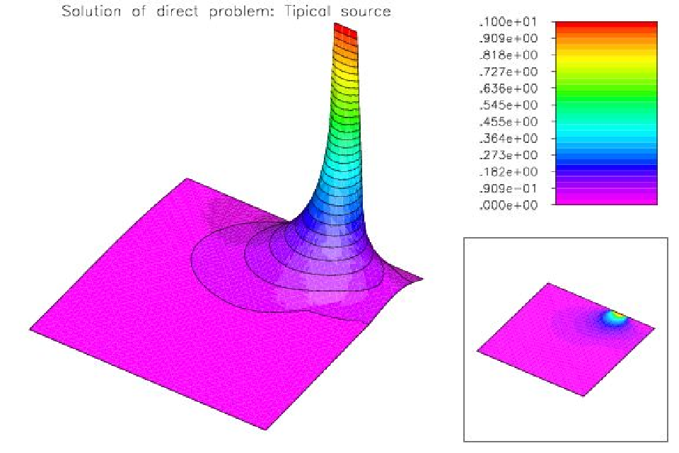
Figure 6: In the top left picture, the doping profile to be identified. In the top right picture, a typical voltage profile UiU_{i} and the corresponding solution uu of (34) - (36). The initial guess used for the l-SDK, l-LK and LK iterative methods is shown in the bottom picture. The boundary parts Γ0\Gamma_{0} and Γ1\Gamma_{1} correspond to the top right and to the lower left edge respectively (the origin is the right corner).

Due to the nature of the practical experiments that can be performed on a factory environment, some restrictions on the data have to be taken into account:

  1. 1.

    The voltage profiles U∈H3/2​(∂ΩD)U\in H^{3/2}(\partial\Omega_{D}) must satisfy U⁡(ξ)=0U(\xi)=0 at the contact Γ1\Gamma_{1}.

  2. 2.

    The parameter xx has to be determined from a finite number of measurements, i.e. from the data

    yiδ:=Σx(Ui)∈Y:=ℝ,i=0,…,N−1,y_{i}^{\delta}:=\Sigma_{x}(U_{i})\in Y:=\mathbb{R}\,,\quad i=0,\dots,N-1\,, (37)

    where the Ui∈H3/2​(∂ΩD)U_{i}\in H^{3/2}(\partial\Omega_{D}) are prescribed voltage profiles satisfying Item 1.

Therefore we can model the inverse doping problem with a system of operator equations of the form (2), namely

Fi(x)=yiδ,i=0,…,N−1,\mathrm{F}_{i}(x)=y_{i}^{\delta}\,,\quad i=0,\dots,N-1\,,

where x∈L2​(Ω)=:Xx\in L^{2}(\Omega)=:X is the unknown parameter, yiδ∈ℝ=:Yy_{i}^{\delta}\in\mathbb{R}=:Y denote the measured data, Fi:X→Y\mathrm{F}_{i}:X\to Y defined by Fi​(x):=Σx​(Ui)\mathrm{F}_{i}(x):=\Sigma_{x}(U_{i}) are the parameter to output maps, with domains of definition

Di:={x∈L∞(Ω): 0<xmin≤x≤xmax, a.e.}.D_{i}:=\{x\in L^{\infty}(\Omega):\,0<x_{\rm min}\leq x\leq x_{\rm max},\mbox{ a.e.}\}\,.

It is worth mentioning that, although the operators Fi\mathrm{F}_{i} are Fréchet differentiable, they do not satisfy the tangential cone condition (11). Therefore, the convergence results derived in Section 3 cannot be applied.

Refer to caption   Refer to caption

Refer to caption   Refer to caption

Refer to caption   Refer to caption

Figure 7: Comparison between the l-SDK, l-LK and LK methods. The top two pictures show the iterative errors obtained by the l-SDK iteration after 10 and 81 cycles. The two central pictures show the iterative errors obtained by the l-LK iteration after 80 and 121 cycles. The two bottom pictures show the iterative errors obtained by the LK after 120 and 380 cycles.

In the following numerical examples we assume that N=11N=11 Dirichlet–Neumann pairs (Ui,Fi​(x′))(U_{i},\mathrm{F}_{i}(x^{\prime})) of measurement data are available. The fixed inputs UiU_{i}, are chosen to be piecewise constant functions supported in Γ0\Gamma_{0},

Ui​(s):={1|s−si|≤h0else,U_{i}(s)\ :=\ \left\{\begin{array}[]{rl}1&|s-s_{i}|\leq h\\ 0&{\rm else}\end{array}\right.\,,

where the points sis_{i} are uniformly distributed on Γ0\Gamma_{0} and h=1/32h=1/32. The doping profile to be reconstructed is shown in Figure 6 (top left picture). The top right picture of Figure 6 shows a typical voltage profile UjU_{j} (applied at Γ0\Gamma_{0}) as well as the corresponding solution uu of (34) - (36). In these pictures, as well as in the forthcoming ones, Γ1\Gamma_{1} appears on the lower left edge and Γ0\Gamma_{0} on the top right edge (the origin corresponds to the upper right corner).

In Figure 7 we show the evolution of the iteration error for the l-SDK, l-LK and LK methods. The same initial guess was used for the three methods (see Figure 6). In our computations we chose τ=2.5\tau=2.5 in (14). The stopping rule for the l-SDK method is satisfied after 81 cycles. For the l-LK method, the same stopping criteria is reached only after 121 cycles. In order to obtain the same accuracy with the LK method, 380 cycles are required. In the top pictures of Figure 7 one can see the iteration error for the l-SDK method after 10 and 81 cycles. For comparison purposes, the iteration error for the l-LK method is shown after 80 and 121 cycles (see the central pictures of Figure 7). The bottom pictures of Figure 7 show the iteration error for the LK method after 120 and 380 cycles. The number of actually computed iterative steps within each cycle of the l-SDK and l-LK methods is shown in Figure 8.

Refer to caption

Figure 8: Comparison between the performance of l-SDK and l-LK methods. The solid (blue) line shows the actually performed number of steps within each cycle of the l-SDK method, while the dashed (red) line gives the corresponding information with respect to the l-LK method.

As one can see in Figure 8, no more than 2 steepest descent steps per cycle are computed after the 1414-th cycle of the l-SDK method. Analogously, no more than 2 Landweber steps per cycle are computed after the 3737-th cycle of the l-LK method. In total, for the computation of the LK-approximation in Figure 7 (380 cycles), 4180 Landweber steps are needed, while the l-LK-approximation (121 cycles) requires the computation of 258 Landweber steps and the l-SDK-approximation (81 cycles) requires the computation of 184 steepest descent steps. The l-LK method requires almost 50% more cycles than the l-SDK method in order to reach the stopping criteria (8). Moreover, the LK method requires almost three times more cycles than the l-LK method in order to achieve the same accuracy (see [10] for other comparisons between the LK and l-LK methods).

The efficiency of the l-SDK method becomes even more evident when we compare the total number of actually performed iterative steps. Each cycle of the LK method requires the computation of 11 steps, while in the l-SDK and l-LK methods the number of actually performed steps per cycle is very small after a few number of cycles.

6 Conclusions

In this paper we propose a new iterative method for inverse problems of the form (2), namely the l-SDK method. As a by-product we also formulated the SDK iteration, which is the steepest descent counterpart of the LK method [17]. In the l-SDK iteration we omit an update of the SDK iteration (within one cycle) if corresponding ii-th residual is below some threshold. Consequently, the l-SDK method is not stopped until all residuals are below the specified threshold. We provided a complete convergence analysis for the l-SDK iteration, proving that it is a convergent regularization method in the sense of [7].

The abstract theory was applied to thermoacoustic computed tomography and an inverse problem for semiconductors. In both applications the l-SDK method turned out to be an efficient iterative regularization method.

Acknowledgments

The work of M.H. and O.S. is supported by the FWF (Austrian Science Fund) grants Y–123INF and P18172–N02. The work of A.L. and A.DC. are supported by the Brazilian National Research Council CNPq, grants 306020/2006–8 and 474593/2007–0. The authors thank Andreas Rieder for stimulating discussion on iterative regularization methods.

References

  • [1] A. B. Bakushinsky and M. Y. Kokurin, Iterative methods for approximate solution of inverse problems, Mathematics and Its Applications, vol. 577, Springer, Dordrecht, 2004.
  • [2] M. Burger, H. W. Engl, A. Leitão, and P. A. Markowich, On inverse problems for semiconductor equations, Milan Journal of Mathematics 72 (2004), 273–313.
  • [3] M. Burger, H. W. Engl, P. A. Markowich, and P. Pietra, Identification of doping profiles in semiconductor devices, Inverse Problems 17 (2001), no. 6, 1765–1795.
  • [4] M. Burger and B. Kaltenbacher, Regularizing newton-kaczmarz methods for nonlinear ill-posed problems, SIAM Journal on Numerical Analysis 44 (2006), 153–182.
  • [5] Y. Censor, P. P. B. Eggermont, and D. Gordon, Strong underrelaxation in kaczmarz’s method for inconsistent systems, Numerische Mathematik 41 (1983), 83–92.
  • [6] P. P. B. Eggermont, G. T. Herman, and A. Lent, Iterative algorithms for large partitioned linear systems, with applications to image reconstruction, Linear Algebar and Applications 40 (1981), 37–67. MR 84c:65059
  • [7] H. W. Engl, M. Hanke, and A. Neubauer, Regularization of inverse problems, Kluwer Academic Publishers, Dordrecht, 1996.
  • [8] D. Finch and Rakesh, The spherical mean value operator with centers on a sphere, Inverse Problems 23 (2007), no. 6, S37–S49.
  • [9] M. Haltmeier and T. Fidler, Frequency domain reconstruction in photo- and thermoacoustic tomography with line detectors, arXiv:math.AP/0610155 (2007), submitted.
  • [10] M. Haltmeier, R. Kowar, A. Leitão, and O. Scherzer, Kaczmarz methods for regularizing nonlinear ill-posed equations. II. Applications, Inverse Problems and Imaging 1 (2007), no. 3, 507–523.
  • [11] M. Haltmeier, A. Leitão, and O. Scherzer, Kaczmarz methods for regularizing nonlinear ill-posed equations. I. convergence analysis, Inverse Problems and Imaging 1 (2007), no. 2, 289–298.
  • [12] M. Hanke, Conjugate gradient type methods for ill-posed problems, Longman Scientific & Technical, 1995.
  • [13] M. Hanke, A. Neubauer, and O. Scherzer, A convergence analysis of Landweber iteration for nonlinear ill-posed problems, Numerische Mathematik 72 (1995), 21–37.
  • [14] M. R. Hestenes and E. Stiefel, On the convergence of the conjugate gradient method for singular linear operator equations., Journal of research of the National Bureau of Standards 49 (1952), 409Ð436.
  • [15] S. Kaczmarz, Approximate solution of systems of linear equations, International Journal of Control 57 (1993), no. 6, 1269–1271, Translated from the German.
  • [16] B. Kaltenbacher, A. Neubauer, and O. Scherzer, Iterative regularization methods for nonlinear ill–posed problems, de Gruyter, 2008, to appear.
  • [17] R. Kowar and O. Scherzer, Convergence analysis of a landweber-kaczmarz method for solving nonlinear ill-posed problems, Ill posed and inverse problems (book series) 23 (2002), 69–90.
  • [18] P. Kuchment and Kunyansky L. A., Mathematics of thermoacoustic and photoacoustic tomography, European Journa of Applied Mathematics (2007), at press.
  • [19] L. Landweber, An iteration formula for Fredholm integral equations of the first kind, American Journal of Mathematics 73 (1951), 615–624.
  • [20] A. Leitao, P. A. Markowich, and J. P. Zubelli, On inverse dopping profile problems for the stationary voltage-current map, Inverse Problems 22 (2006), 1071–1088.
  • [21] A. K. Louis and E. T. Quinto, Local tomographic methods in sonar, Surveys on solution methods for inverse problems, Springer, Vienna, 2000, pp. 147–154.
  • [22] S. McCormick, The methods of Kaczmarz and row orthogonalization for solving linear equations and least squares problems in Hilbert space, Indiana University Mathematics Journal 26 (1977), 1137–1150.
  • [23] V. A. Morozov, Regularization methods for ill–posed problems, CRC Press, Boca Raton, 1993.
  • [24] F. Natterer, Algorithms in tomography, State of the Art in Numerical Analysis, vol. 63, 1997, pp. 503–524.
  • [25]   , The mathematics of computerized tomography, SIAM, Philadelphia, 2001.
  • [26] F. Natterer and F. Wübbeling, Mathematical Methods in Image Reconstruction, SIAM, Philadelphia, 2001.
  • [27] G. Paltauf, R. Nuster, M. Haltmeier, and P. Burgholzer, Experimental evaluation of reconstruction algorithms for limited view photoacoustic tomography with line detectors, Inverse Problems 23 (2007), no. 6, S81–S94.
  • [28]   , Photoacoustic tomography using a mach–zehnder interferometer as acoustic line detector, Applied Optics (2007), 3352–3358.
  • [29] O. Scherzer, A convergence analysis of a method of steepest descent and a two-step algorithm for nonlinear ill-posed problems, Numerical Functional Analysis and Optimization 17 (1996), no. 1-2, 197–214.
  • [30] T. I. Seidman and C. R. Vogel, Well posedness and convergence of some regularisation methods for non–linear ill posed problems, Inverse Problems 5 (1989), 227–238.
  • [31] J. R. Shewchuck, An introduction to the conjugate gradient method without the agonizing pain, Tech. report, Scholl of Computer Science, Carnegie Mellon University, 1994.
  • [32] A. N. Tikhonov, Regularization of incorrectly posed problems, Soviet Math. Dokl. 4 (1963), 1624–1627.
  • [33] A. N. Tikhonov and V. Y. Arsenin, Solutions of ill-posed problems, John Wiley & Sons, Washington, D.C., 1977, Translation editor: Fritz John.
  • [34] M. Xu and L. V. Wang, Photoacoustic imaging in biomedicine, Review of Scientific Instruments 77 (2006), no. 4, 041101.
  • [35] Y. Xu, L.V. Wang, G. Ambartsoumian, and P. Kuchment, Reconstructions in limited-view thermoacoustic tomography, Medical Physics 31 (2004), no. 4, 724–733.