Proton elastic scattering from tin isotopes at 295 MeV and systematic change of neutron density distributions

S. Terashima¹, H. Sakaguchi¹, H. Takeda^1∗, T. Ishikawa¹, M. Itoh¹, T. Kawabata¹, T. Murakami¹, M. Uchida¹, Y. Yasuda¹, M. Yosoi^1,2, J. Zenihiro¹, H. P. Yoshida^2§, T. Noro³, T. Ishida^3‡, S. Asaji³, T. Yonemura³ Note: Present address: RIKEN Nishina Center, Wako, Saitama 351-0198, Japan Note: Present address: Miyazaki University, Miyazaki, Miyazaki 889-2192, Japan Note: Present address: Laboratory of Nuclear Science, Tohoku University, Sendai, Miyagi 982-0216, Japan Note: Present address: Cyclotron and Radioisotope Center, Tohoku University, Sendai, Miyagi 980-8578, Japan Note: Present address : Center for Nuclear Study, University of Tokyo, Wako, Saitama 351-0198, Japan Note: Present address : Tokyo Institute of Technology, Ookayama, Tokyo 152-8550, Japan Note: Present address : University of Tsukuba, Tsukuba, Ibaraki 305-8571, Japan Address: ¹Department of Physics, Kyoto University, Kyoto 606-8502, Japan
² Research Center for Nuclear Physics (RCNP), Osaka University, Osaka 567-0047, Japan
³ Department of Physics, Kyushu University, Fukuoka 812-8581 Japan

August 24, 2026

Abstract

Cross sections and analyzing powers for proton elastic scattering from ^{116,118,120,122,124}Sn at 295 MeV have been measured for a momentum transfer of up to about 3.5 fm^-1 to deduce systematic changes of the neutron density distribution. We tuned the relativistic Love-Franey interaction to explain the proton elastic scattering of a nucleus whose density distribution is well known. Then, we applied this interaction to deduce the neutron density distributions of tin isotopes. The result of our analysis shows the clear systematic behavior of a gradual increase in the neutron skin thickness of tin isotopes with mass number.

pacs

21.10.Gv, 21.30.Fe, 24.10.Jv, 27.60.+j

I Introduction

Charge distributions in stable nuclei have been reliably measured by electron elastic scattering and muonic x-ray data [1]. These charge-sensitive experiments have provided precise information on charge distributions. On the other hand, it is much more difficult to deduce neutron density distributions, since electromagnetic interaction provides little information on neutron density distributions. The proton and neutron density distributions have a similar shape in stable nuclei. However in recent research it has been reported that in some unstable nuclei the differences between proton and neutron shapes are greater than those in stable nuclei [2]. It has also been indicated that the thickness of the neutron skin is closely related to the symmetry term of the equation of state (EOS) [3, 4]. Thus, the determination of neutron density distributions has become increasingly important.

There have been many experiments attempting to extract neutron and matter density distributions in the nuclear interior using hadronic probes [5]. Pion and alpha elastic scattering have been performed in the study of neutron and matter density distributions [6, 7, 8]. Compared with other hadronic probes, the elastic scattering of protons at intermediate energies is suitable for extracting information on the nuclear surface and interior, because at intermediate energies, proton elastic scattering has a simple reaction mechanism. To deduce nuclear densities using protons, the incident energy has to be sufficiently high to describe the scattering by the simple mechanism. At energies above 100 MeV, we can explain proton elastic scattering microscopically, because the imaginary part of the optical potential describes a quasi-free process mainly without the need for a renormalization factor. So far, energies above 500 MeV have been applied for proton elastic scattering to study neutron density distributions [9, 10]. However, this energy is sufficiently high to produce mesons, and information on the nuclear interior is easily masked by the meson-productions. Furthermore, the total cross section of nucleon-nucleon scattering shows a minimum at the incident energy of 300 MeV. We thus adopt 300 MeV protons in this work as probes for information on the nuclear interior.

In our previous papers [11], we tuned the effective relativistic Love-Franey interaction by introducing ’so-called medium effects’ for the scattering from a nucleus whose density distribution is well known. We used elastic scattering from ⁵⁸Ni to tune the interaction, since ⁵⁸Ni is the heaviest stable nucleus with N $\approx$ Z and the density distribution of the neutrons in ⁵⁸Ni can be assumed to be the same as that for the protons. To explain the results of our experiments we found that we had to modify the scattering amplitudes of the nucleon-nucleon interactions inside the nucleus as follows. We phenomenologically changed the masses and coupling constants of exchanged mesons depending on the nuclear density. Thus, we could explain the scattering sufficiently well to deduce the matter density distribution precisely.

For our first systematic search for neutron density distributions, we selected tin isotopes. Tin has many stable isotopes (¹¹²Sn-¹²⁴Sn). Also, unstable tin isotopes have a long isotopic chain including two double-magic nuclei (¹⁰⁰Sn [N=50], ¹³²Sn [N=82]). Moreover, its proton number is a magic number (Z=50). Thus, tin isotopes are suitable for the study of systematic changes in neutron density distributions. The main purposes of this work are to attempt to deduce information on neutron density distributions, and to systematically study the neutron skin thickness of tin isotopes. The experimental setup and procedure are described in Sec. II. Details of the analysis used to deduce neutron density distributions are given in Sec. III. The deduced radii of tin isotopes are discussed in Sec. IV.A summary is given in Sec. V.

II Experiment

The measurements were performed at the Research Center for Nuclear Physics (RCNP), Osaka University. Polarized protons from a high-intensity polarized ion source were injected into an AVF cyclotron, transported to a six-sector ring cyclotron and accelerated up to 295 MeV. The polarization axis was in the vertical direction. The spin direction and magnitude of the beam polarization were measured continuously using sampling-type beam-line polarimeters (BLPs) [12] placed between the ring cyclotron and a scattering chamber. Each polarimeter utilized left-right asymmetries in p-H scattering from (CH₂)_n foil to determine the vertical transverse component $p_{y}$ of the beam polarization. The typical beam polarization was 65%. Then the beam was transported to a target center in the scattering chamber. The typical beam spot size on the target during measurements was 1 mm in diameter. Finally, the beam was stopped by an internal Faraday cup inside the scattering chamber in the case of forward-angle measurements. In the measurements at backward scattering angles, the beam was transported to another Faraday cup located inside the shielding wall of the experimental room about 25 m downstream of the scattering chamber. The integrated beam current was monitored using a current digitizer (Model 1000C) made by BIC (Brookhaven Instruments Corporation). Additionally, the beam current was monitored independently using p-p cross sections at the BLPs during the backward-angle measurements. Five tin isotope targets (^{116,118,120,122,124}Sn) in the form of self-supporting metal foils were used for this experiment. Two different thicknesses were used for each target. Thin targets were used for the forward-angle measurements to reduce the dead time of the data acquisition system, and thick targets were for the backward-angle measurements to increase the yields. The enrichment and thicknesses of each target are shown in Table 1.

Table 1: Target enrichment and thicknesses of tin isotopes.

Nucleus	Enrichment	Thin	Thick
¹¹⁶Sn	95.5 $\%$	10.0mg/cm²	100.mg/cm²
¹¹⁸Sn	95.8 $\%$	10.0mg/cm²	100.mg/cm²
¹²⁰Sn	98.4 $\%$	5.12mg/cm²	39.9mg/cm²
¹²²Sn	93.6 $\%$	10.5mg/cm²	85.4mg/cm²
¹²⁴Sn	95.5 $\%$	5.00mg/cm²	62.7mg/cm²

The main contaminants of the targets originated from other tin isotopes. The present energy resolution could not separate the elastic scattering of other tin isotopes. Thus, we analyzed the targets including the contamination from other isotopes at all momentum transfer regions. We estimated the error of this analysis to be less than 1 $\%$ for all cross sections and analyzing powers. We used an automatic target changer system in this experiment to reduce the systematic errors of relative cross sections between isotopes. We formed a stack of three targets, which were moved vertically every 2 min to avoid errors due to the drift of the beam direction and that of its position on the targets.

We used a high-resolution (p/ $\Delta$ p $\sim$ 37,000) magnetic spectrometer, ’Grand Raiden’ (GR), which had a Q1-SX-Q2-D1-MX-D2 configuration and focal-plane counters for momentum analysis [13]. The focal-plane counters consisted of two vertical-drift-type multi wire drift chambers (VDCs) and two plastic scintillating counters. The momentum of protons scattered from the target was analyzed using the GR. The trajectory of the scattered protons from the target was reconstructed from the position measurement carried out using two sets (X1,U1 and X2,U2) of VDCs, which were placed near the focal plane of the spectrometer [14]. Each set had an effective area of 120 cm [width] $\times$ 10 cm [height]. Two 1 cm-thick plastic scintillating counters (PS1 and PS2) placed behind the VDCs were used as triggers and for particle identification.

The energy resolution of the beam was 200 keV in FWHM, which was determined by the energy width of the beam itself and was sufficient to separate elastic peaks from inelastic peaks. Figure 1 shows a sample focal-plane spectra of ¹²⁰Sn. The differential cross sections and analyzing powers were measured for analysis of up to 50^∘, corresponding to a momentum transfer of 3.5 fm^-1 in the center-of-mass system. We included 3% errors for both cross sections and analyzing powers as errors resulting from experimental conditions including target thickness uncertainty.

Refer to caption — Figure 1: Sample focal plane spectra corresponding to the excitation energy of ¹²⁰Sn, taken at a laboratory scattering angle of 35.5^∘

III Theoretical Analysis

We analyzed our data using the formula for the relativistic impulse approximation (RIA) using the relativistic Love-Franey interaction [15]. The invariant amplitude has been determined from nucleon-nucleon phase shifts and is expressed as

	$\displaystyle F(q)$	$\displaystyle=$	$\displaystyle F^{S}+F^{V}\gamma^{\mu}_{(0)}\gamma^{\mu}_{(1)}+F^{PS}\gamma^{5}_{(0)}\gamma^{5}_{(1)}$		(1)
			$\displaystyle+F^{T}\sigma^{\mu\nu}_{(0)}\sigma_{(1)\mu\nu}+F^{A}\gamma^{5}_{(0)}\gamma^{\mu}_{(0)}\gamma^{5}_{(1)}\gamma_{(1)\mu}.$		(1)

Each amplitude is shown as the sum of real and imaginary amplitudes using the masses, coupling constants, and cutoff parameters of exchanged mesons.

Figure 2 shows the experimental results for five tin isotopes and two different theoretical results. The solid lines in Fig. 2 are the results of RIA calculations with the default parameters proposed by Murdock and Horowitz [15]and the relativistic mean field (RMF) densities [16]. The dashed lines are the calculations using the global potential [17, 18]. While both calculations are in good agreement with the experimental data of obtained from the analyzing powers, the differential cross sections are overestimated, particularly in the large-momentum-transfer region. Murdock and Horowitz used different masses and coupling constants for real and imaginary scattering amplitudes, depending on the interaction. In our previous work, we attempted to explain the experimental data by phenomenologically changing the masses and coupling constants of exchanged mesons ( $\sigma,\omega$ ) in the real and the imaginary amplitudes depending on the nuclear density. The formula for density dependence is as follows;

	$\displaystyle g_{j}^{2},\bar{g}_{j}^{2}$	$\displaystyle\longrightarrow$	$\displaystyle\frac{g_{j}^{2}}{1+a_{j}~\rho(r)/\rho_{0}},\frac{\bar{g}_{j}^{2}}{1+\bar{a}_{j}~\rho(r)/\rho_{0}}$
	$\displaystyle m_{j},\bar{m}_{j}$	$\displaystyle\longrightarrow$	$\displaystyle{m_{j}}[1+b_{j}~\rho(r)/\rho_{0}],{\bar{m}_{j}}[1+\bar{b}_{j}~\rho(r)/\rho_{0}],$		(2)

where, $m_{j},\bar{m}_{j},g_{j}$ , and, $\bar{g}_{j}$ indicate the masses, and coupling constants of mesons for real and imaginary amplitudes, respectively, where j refers to the $\sigma,\omega$ mesons. The normal density $\rho_{0}$ is 0.1934 fm^-3 [11, 19]. These changes in the masses and coupling constants are called medium effects, and may be an effect of the presentations of the partial restoration of chiral symmetry, Pauli blocking, and multistep processes. The tuned effective interaction is applied to existing ²⁰⁸Pb data obtained at TRIUMF [20] with a density distribution calculated from the RMF in Fig. 3. It was found that the tuning of the effective interaction was meaningfully improved compared with the original unmodified interaction.

For the RIA calculation, we need four density distributions; the vector and scalar density distributions of protons and neutrons. The proton density distribution and the relation between the scalar and vector density can be obtained from the charge distributions, the nucleon electric form factors, and the RMF calculation. Thus, we can determine the neutron density distribution by comparing experimental data with a calculation using the tuned effective interaction.

In this paper, we attempt to extract neutron density distributions for tin isotopes, considering the various ambiguities caused by the modification parameters used in the RIA calculation, the proton form factors, and an assumption based on scalar densities.

III.1 Proton density distributions of tin isotopes

For the RIA calculations we used point proton density distributions derived from charge distributions observed in electron-scattering experiments [1]. We used the sum-of-Gaussian-type (SOG) charge distributions of ^116,124Sn, which were obtained from the electron scattering over a 3.5-fm^-1-wide momentum transfer region [21]. The charge distributions are described as

	$\displaystyle\rho_{ch}(r)$	$\displaystyle=$	$\displaystyle\frac{Z}{2\pi^{3/2}\gamma^{3}}\sum_{i=1}^{12}\frac{Q_{i}}{1+2R_{i}^{2}/\gamma^{2}}$		(3)
			$\displaystyle\times\left[e^{-(r-R_{i})^{2}/\gamma^{2}}+e^{-(r+R_{i})^{2}/\gamma^{2}}\right].$		(3)

However, reported data on charge distributions obtained using model-independent distributions are limited.

Figure 4 shows existing experimental results for the charge radius of tin isotopes. Since the radius of tin isotopes increases smoothly with mass number and the number of protons is constant, we can expect a smooth change in the charge distributions as the neutron number increases. Thus we obtained the charge distributions of ^118,120,122Sn by interpolation using the arithmetic mean of the previous derived charge distributions of ^116,124Sn;

$\displaystyle\rho_{ch}^{{}^{118}{\it Sn}}(r)$	$\displaystyle=$	$\displaystyle\frac{3\rho_{ch}^{{}^{116}{\it Sn}}(r)+\rho_{ch}^{{}^{124}{\it Sn}}(r)}{4}$	(4)
$\displaystyle\rho_{ch}^{{}^{120}{\it Sn}}(r)$	$\displaystyle=$	$\displaystyle\frac{\rho_{ch}^{{}^{116}{\it Sn}}(r)+\rho_{ch}^{{}^{124}{\it Sn}}(r)}{2}$	(5)
$\displaystyle\rho_{ch}^{{}^{122}{\it Sn}}(r)$	$\displaystyle=$	$\displaystyle\frac{\rho_{ch}^{{}^{116}{\it Sn}}(r)+3\rho_{ch}^{{}^{124}{\it Sn}}(r)}{4}.$	(6)

The interpolated radii of model-independent-type charge distributions for ^118,120,122Sn are consistent with other experimental data obtained from the electron scattering [1] and muonic x-rays [23], as shown in Fig. 4. The differences between interpolated radii and other results from the combined analyses of elastic electron scattering and muonic x-ray data elastic electron scattering and muonic x-ray data are small [22]. We estimate that the errors of our deduced charge radii are 0.003 fm, which are the same order as those for ^116,124Sn

To extract the point proton density distribution we need to unfold the charge distribution with the finite size of the protons and to consider the contribution from neutrons. Therefore, we can write a charge distribution $\rho_{ch}$ using the charge distributions of a proton $\rho_{ch}^{proton}$ and neutron $\rho_{ch}^{neutron}$ as follows;

	$\displaystyle\rho_{ch}(\vec{r})$	$\displaystyle=$	$\displaystyle\int\rho_{p}(\vec{r^{\prime}})\rho^{proton}_{ch}(\vec{r}-\vec{r^{\prime}})d\vec{r^{\prime}}$		(7)
			$\displaystyle+\int\rho_{n}(\vec{r^{\prime\prime}})\rho^{neutron}_{ch}(\vec{r}-\vec{r^{\prime\prime}})d\vec{r^{\prime\prime}}.$		(7)

Therefore, we calculate the mean square radius of the charge distribution as follows;

\displaystyle\left<r^{2}_{ch}\right>

\displaystyle=

\displaystyle\left<r^{2}_{p}\right>+\left<(r_{ch}^{proton})^{2}\right>+\frac{N}{Z}\left<(r_{ch}^{neutron})^{2}\right>,

(8)

where

$\displaystyle\left<r^{2}_{ch}\right>$	$\displaystyle\equiv$	$\displaystyle\int r^{2}\rho_{ch}(\vec{r})d\vec{r}/\int\rho_{ch}(\vec{r})d\vec{r}$
$\displaystyle\left<r^{2}_{p}\right>$	$\displaystyle\equiv$	$\displaystyle\int r^{2}\rho_{p}(\vec{r})d\vec{r}/\int\rho_{p}(\vec{r})d\vec{r}$
$\displaystyle\left<(r^{proton}_{ch})^{2}\right>$	$\displaystyle\equiv$	$\displaystyle\int r^{2}\rho^{proton}_{ch}(\vec{r})d\vec{r}/\int\rho^{proton}_{ch}(\vec{r})d\vec{r}$
$\displaystyle\left<(r^{neutron}_{ch})^{2}\right>$	$\displaystyle\equiv$	$\displaystyle\int r^{2}\rho^{neutron}_{ch}(\vec{r})d\vec{r}/\int\rho^{neutron}_{ch}(\vec{r})d\vec{r}.$

$\left<r_{ch}^{2}\right>^{1/2},\left<r_{p}^{2}\right>^{1/2},\left<(r_{ch}^{proton})^{2}\right>^{1/2},{\rm and}\left<(r_{ch}^{neutron})^{2}\right>^{1/2}$ are denoted as the root-mean-square (RMS) radii of $\rho_{ch}$ , $\rho_{p}$ , $\rho_{ch}^{proton}$ , and $\rho_{ch}^{neutron}$ , respectively. We used the simple parameterization of nucleon form factors [24], where the RMS radius of the proton itself is 0.863(4) fm and the mean square radius of the neutron itself is -0.112(3) fm². This proton radius is consistent with that obtained from the measurement of the hydrogen 1S Lamb shift [25]. The contribution to the RMS radius of the point proton density distribution from the neutron form factor is in the order of 0.02 fm. Thus, the contribution from the neutron form factor is small but not negligible.

Equation (7) shows that we need the neutron density distribution to precisely deduce density distribution. Since the errors of proton radii are mainly determined by the charge radii in the equation, the errors of the RMS radii of the point proton of tin isotopes are estimated to be 0.003 fm.

In this report we tune newly a medium-effect parameter set using the ⁵⁸Ni data of Refs. [11, 26], because we adopted a new treatment for the point proton density distribution.

III.2 ⁵⁸Ni and the effective interaction

We must calibrate the effective nucleon-nucleon interaction, particularly in the nuclear interior, by the scattering from the nucleus. In this subsection we discuss the analysis of the elastic scattering of ⁵⁸Ni at the energy of 295 MeV, which allows to adjust the effective interaction further.

In the previous work, eight parameters were searched for independently including the imaginary parts of two exchanged mesons [11]. It is difficult to obtain a unique medium-effect parameter set due to its many degrees of freedom. This difficulty causes ambiguities in the neutron density distributions. Thus, we attempt to express the elastic scattering using the medium-effect parameters that have less freedom. We need the information of both proton and neutron density distributions to calibrate the effective interaction based on RIA calculations. Several calculations have been performed to obtain the proton and neutron density distributions of ⁵⁸Ni using relativistic or nonrelativistic mean-field calculations. The results are dependent on the interactions used in the calculations but the differences between the RMS radii of point protons and neutrons, the neutron skin, are generally small [30, 31, 32, 29, 27, 28], and are given as

\Delta r_{np}\equiv\left<r_{n}^{2}\right>^{1/2}-\left<r_{p}^{2}\right>^{1/2}.

(9)

The used of 800MeV proton elastic scattering based on KMT nonrelativistic impulse approximation gave a thickness of $\Delta r_{np}$ =0.01(5) fm [9]. X-ray measurement of an antiprotonic atom gave a value of -0.9(9) fm [33]. Thus, in the case of ⁵⁸Ni, we can assume that the neutron density distribution has the same shape as the proton density distribution. Therefore, the neutron density distribution can be described as

\rho_{n}(r)=(N/Z)\rho_{p}(r).

(10)

Thus, the substitution of Eq. (10) into Eq. (7) gives Eq. (11) the point proton density distribution of ⁵⁸Ni,

	$\displaystyle\rho_{ch}(\vec{r})$	$\displaystyle=$	$\displaystyle\int\rho_{p}(\vec{r}^{\prime})[\rho^{proton}_{ch}(\vec{r}-\vec{r}^{\prime})$		(11)
			$\displaystyle+(N/Z)\rho^{neutron}_{ch}(\vec{r}-\vec{r}^{\prime})]d\vec{r}^{\prime}.$		(11)

According to the RMF calculation, the ratio of scalar-to-vector densities has an almost constant value of 0.96, as shown in Fig. 5, corresponding to the ratio of the integrated scalar density to the integrated vector density. Using this constant value, we reproduced the scalar density distributions from the RMF calculation.

Even if we had taken different constant value from 0.95 to 0.97, the differences in the cross sections and analyzing powers would have been less than 2-3%, which can be compensated for by the ambiguity of the medium-effect parameters.

Since in the case of eight parameters, we have too many degrees of freedom for fitting parameters and the correlations among these parameters are large, in this work we have used the same modification parameters for both real and imaginary parts of the scattering amplitude ( $\bar{\rm a}_{j}$ =a_j , $\bar{\rm b}_{j}$ =b_j). Figure 6 shows the correlation between modification parameters of a_σ and a_ω. The correlation is valley like and very strong; the correlations of the other five combinations of modification parameters also show similar behavior. Thus, we determined the modification parameters uniquely.

The medium-effect parameters were determined by fitting the experimental data so as to minimize the chi-square ( $\chi^{2}$ ) value. $\chi^{2}$ is defined as

\chi^{2}=\sum\left[(x_{exp.}-x_{theo.})/\Delta x_{exp.}\right]^{2}

(12)

where x_exp., $\Delta x_{exp.}$ and x_theo. are the experimental data, the errors in the data, and the calculation results, respectively. Figure 7 shows the experimental data at 295 MeV and the fits with the RIA calculation using the modified effective interaction with the unfolded proton and neutron densities of ⁵⁸Ni obtained using Eq. (10). Our calculations are in good agreement with all the data of the cross sections, the analyzing powers, and the spin rotation parameters for up to 3.5 fm^-1. $\chi^{2}_{min}$ , the minimum of $\chi^{2}$ for ⁵⁸Ni data using four free parameters, has almost the same order as that in the previous work using eight free parameters. We estimated the errors of the modification parameters from the statistics and the experimental conditions as follows.

\displaystyle\chi^{2}\leq\chi^{2}_{min}+P

(13)

Here, P (in this work P=4) denotes a number of fitting parameters [34]. Table 2 shows a summary of the fitting results.

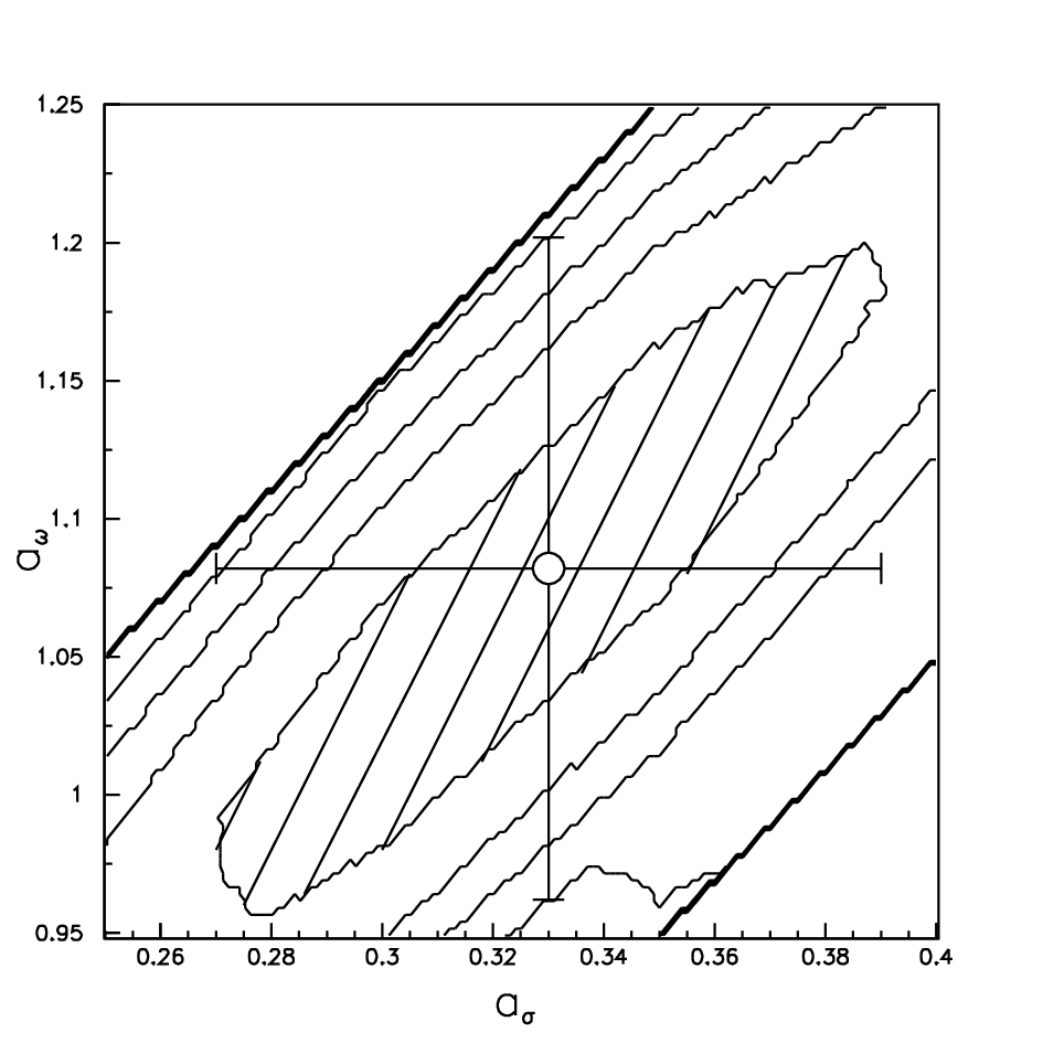
Figure 6 shows the correlation between a_σ and a_ω. The circle shows the best-fit parameter, and horizontal and vertical bars show the error bars of a_σ and a_ω, respectively. The hatched area shows the region that satisfies Eq. (13). Since each pair of parameters has a strong correlation, we cannot independently use the entire region defined by the errors in Table 2, meaning that the usable area defined by each pair of the parameter set is very narrow.

Table 2: Medium-effect parameters at 295 MeV. The error estimation is discussed in Sec. II.B

$j$	$\sigma$	$\omega$
$a_{j}$	0.33 $\pm$ 0.06	1.08 $\pm$ 0.12
$b_{j}$	-0.12 $\pm$ 0.05	-0.30 $\pm$ 0.03

III.3 Tin isotopes and neutron density distributions

We have tried to deduce the neutron density distributions of tin isotopes using the newly modified effective interaction. The scalar nucleon density distributions of tin isotopes were assumed to be 0.96 times the vector nucleon density distributions as in the case of ⁵⁸Ni, because the ratios of the scalar to vector densities for tin isotopes are almost the same [16]. The initial proton density distributions of tin isotopes are obtained by Eq. (7) using the neutron density distribution given by Eq. (10). We used a SOG for the neutron density distribution, which is expressed as

	$\displaystyle\rho_{n}(r)$	$\displaystyle=$	$\displaystyle\frac{N}{2\pi^{3/2}\gamma^{3}}\sum_{i=1}^{12}\frac{Q_{i}}{1+2R_{i}^{2}/\gamma^{2}}$		(14)
			$\displaystyle\times\left[e^{-(r-R_{i})^{2}/\gamma^{2}}+e^{-(r+R_{i})^{2}/\gamma^{2}}\right].$		(14)

Here, N is the number of neutrons. Equation (14) is almost the same as Eq. (3). While parameters such as $\gamma$ and $R_{i}$ were fixed using results of the charge distribution of ^116,124Sn [1], Q_i were determined independently under the following normalization condition;

\int\rho_{n}(r)dr=N\Rightarrow\sum_{i=1}^{12}Q_{i}=1.

(15)

For fitting, we used a range of momentum transfer from 0.7 fm^-1 to 3.5 fm^-1, since the data for the forward angle ( $\theta_{\rm c.m.}<8^{\circ}$ ) were difficult to measure experimentally. Our range covers the same momentum transfer region of electron scattering as that in Ref. [1]. For the medium-effect parameters, we used the same parameters as those determined by the scattering from the ⁵⁸Ni target.

In Fig. 8, we show experimental data together with the fitting results and calculations using the initial neutron density distributions, which are defined as

\rho_{n}(r)=\rho_{p}(r)+(\rho_{n}^{RMF}(r)-\rho_{p}^{RMF}(r)),

(16)

where $\rho_{n(p)}^{RMF}(r)$ denote the RMF neutron (proton) density distributions [16]. We determine the proton and neutron density distributions by iterating Eq. (7) several times until self-consistency is achieved. The process of iteration hardly affects the proton densities, because the proton density distributions are not sensitive to the fine structure of the neutron density distributions.

The calculations using the initial neutron density and the medium-modified effective interaction reproduce the absolute value of the cross sections and analyzing powers. The angular distributions of both the differential cross sections and the analyzing powers using the initial neutron density are shifted to forward angle in angle because the RMF calculation has a tendency of a larger neutron radius.

III.4 Uncertainties of neutron density distributions

We estimated the uncertainties of the neutron density distributions of the tin isotopes. There are generally two types of uncertainty. One originates from the experiment, and the other originates from the model of calculation. In our case, the reduced chi-square $\chi^{2}/\nu$ is larger than 1, and is typically 7 for ^{116,118,122,124}Sn. In the case of ¹²⁰Sn, not only the cross section and analyzing powers but also the spin rotation parameters [26] are used as experimental data in the analysis. Thus, the errors for ¹²⁰Sn resulting from the experimental conditions, degrees of freedom $\nu$ and $\chi^{2}/\nu$ are different from those for other isotopes. $\chi^{2}/\nu$ is about 10 for ¹²⁰Sn. If the model were perfect, it would realize $\chi^{2}/\nu$ =1. Thus, the reason that $\chi^{2}/\nu>$ 1 is attributed to the inadequacy of our model. To compensate for this inadequacy of the model, we increased the errors artificially by multiplying all the experimental errors by a constant factor to realize $\chi^{2}/\nu$ =1. This means that we must redefine Eq. (13) as follows;

\displaystyle\chi^{2}\leq\chi^{2}_{min}+P\times{\chi}^{2}_{min}/\nu.

(17)

The uncertainties of the neutron density distributions are estimated by the following procedure.

First, we obtain a new medium-effect parameter set using ⁵⁸Ni data by the Monte Carlo method. We adopt the parameter sets that satisfy Eq. (13) as ’good’ medium-effect parameter sets.

Second, we estimate the uncertainties of neutron density distributions using each set of good medium-effect parameters. The neutron density distributions are calculated by the Monte Carlo method under the normalization condition of Eq. (15). We compare the experimental data with the result of the calculation using each good set of medium-effect parameters and the trial neutron density distributions. We also adopt all neutron density distributions that satisfy Eq. (17) as good neutron density distributions.

We repeated this procedure until the uncertainty of each good neutron density distribution converged. The uncertainties of the neutron density distributions in this analysis are defined as the outskirts of the density distributions at each radial point. The uncertainties of the RMS radii of the neutron density distributions were also calculated using all the neutron density distributions that satisfy Eq. (17).

Figure 9 shows the deduced neutron density distributions and point proton density distributions of the tin isotopes. Hatched areas in the figure represent outskirt regions encompassing all the neutron density distributions for tin isotopes allowed by Eq. (17), corresponding to the uncertainties of the neutron density distributions in this analysis.

Table 3 shows a summary of the RMS radii of the proton and neutron density distributions and the neutron skin thicknesses of the tin isotopes.

Table 3: Reduced RMS radii and thicknesses of tin isotopes.

Target	$\left<\rho_{p}^{2}\right>^{1/2}$ (fm)	$\left<\rho_{n}^{2}\right>^{1/2}$ (fm)	$\Delta r_{np}$ (fm)
$\rm{}^{116}Sn$	4.562 $\pm$ 0.003	4.672 $\pm$ 0.018	0.110 $\pm$ 0.018
$\rm{}^{118}Sn$	4.575 $\pm$ 0.003	4.720 $\pm$ 0.016	0.145 $\pm$ 0.016
$\rm{}^{120}Sn$	4.589 $\pm$ 0.003	4.736 $\pm$ 0.033	0.147 $\pm$ 0.033
$\rm{}^{122}Sn$	4.602 $\pm$ 0.003	4.748 $\pm$ 0.016	0.146 $\pm$ 0.016
$\rm{}^{124}Sn$	4.615 $\pm$ 0.003	4.800 $\pm$ 0.017	0.185 $\pm$ 0.017

In the high-momentum-transfer region, the multistep process may affect the angular distribution of elastic scattering [35]. To estimate the effect of multistep processes, we performed a coupled-channel calculation by using the coupled-channel code ECIS95 written by Raynal [36]. Figure 10 shows the calculated cross sections and analyzing powers with and without performing a coupled-channel calculation using the global potential [17, 18]. The contribution from the coupled-channel calculation for ⁵⁸Ni in the momentum transfer range from 0.7 fm^-1 to 3.5 fm^-1 is relatively small (1-2%), which is less than the uncertainty of the medium-effect parameter. In the case of the tin isotopes, the situation is similar to the case of ⁵⁸Ni. Thus, the effect from the coupled channel is masked by the uncertainties of our introduced medium effects in this analysis. Also, the coupled-channel effect might be partly included in our parametrization because we aimed to phenomenologically reproduce the experimental data. Thus, the effect of the coupled-channel is negligible and was not included explicitly in our analysis.

IV Results and Discussion

We have obtained the uncertainties of neutron density distributions considering statistics, systematic experimental errors, the uncertainties of the modification parameters, and our model, as shown in Fig. 9. Therefore the differences among the deduced shapes of the neutron density distributions of tin isotopes gradually changes. However the deduced RMS radii of the point proton and neutron density distributions clearly increase with the mass number, as shown in Fig. 11.

This tendency is also shown in the results of several typical theoretical calculations, which are also plotted in the figure and have slopes consistent with our experimental results. Among the calculations, the nonrelativistic Skyrme Hartree Fock (SHF) calculations using SkM^∗ parametrization are in good agreement with the RMS radii of both point proton and neutron density distributions. Neutron skin thicknesses $\Delta r_{np}$ are shown in Fig. 12. The neutron skin thicknesses are about 0.11-0.19 fm for tin isotopes, which are not large what some RMF models suggest. The values of our $\Delta r_{np}$ are reproduced by the SHF calculation using SkM^∗ parameterization. On the other hand, the values are larger than SIII and smaller than NL3. Oyamatsu et al. and Chen et al. calculated a linear relation between the $\Delta r_{np}$ and the symmetry term of the EOS [40, 41]. Therefore, our results favor medium values for the symmetry energy and its density dependence used in SkM^∗ one, which are not so large as NL3 but larger than SIII.

V Summary

In this work, we have extracted the neutron density distributions of tin isotopes. The experimental data were analyzed in the framework of the RIA using a newly tuned relativistic Love-Franey interaction obtained for ⁵⁸Ni. The uncertainties of the neutron density distributions were estimated in consideration of not only experimental but also model uncertainties. Using the tuned interactions in the nuclear medium, the neutron density distributions of the tin isotopes were deduced so as to reproduce the experimental data of the isotopes. We also deduced the RMS radii of the point proton and neutron density distributions. We compared our experimental results with those of several theoretical mean-field calculations. SHF calculations using SkM^∗ parameterization as above were in good agreement with the RMS radii of both point proton and neutron density distributions. We observed a clear increase in neutron skin thickness with mass number, although the values obtained were not large what some RMF models suggest.

Acknowledgements.

We would like to thank Prof. Hatanaka and the operating crew of RCNP for their support; for providing a clear, stable, and high-intensity beam during the experiment; and also for beam-time management. This experiment was performed at RCNP under program No. E147.

References

[1] H. de Vries, C. W. de Jager and C. de Vries, Atomic Data and Nuclear Data Tables 36, 495 (1987).
[2] I. Tanihata, Nucl. Phys. A488, 113 (1988).
[3] S. Typel and B. A. Brown , Phys. Rev. C 64, 027302 (2001).
[4] P. Danielewicz, Nucl. Phys. A727, 233 (2003).
[5] C. J. Batty et al., in Advances in Nuclear Physics, edited by J. W. Negele and E. Vogt (Plenum, New York, 1989), Vol. 19, p. 1.
[6] H. J. Gils, H. Rebel, E. Friedman, Phys. Rev. C 29, 1295 (1984).
[7] R. R. Johnson et al., Phys. Rev. Lett. 43, 844 (1979).
[8] B. M. Barnett et al., Phys. Lett. B156, 172 (1984).
[9] L. Ray, W. R. Coker and G. W. Hoffmann, Phys. Rev. C 18, 2641 (1978). L. Ray, Phys. Rev. C 19, 1855 (1979).
[10] V. E. Starodubsky and N. M. Hintz, Phys. Rev. C 49, 2118 (1994).
[11] H. Sakaguchi et al., Phys. Rev. C 57, 1749 (1998).
[12] T. Ichihara, H. Sakaguchi, K. Hatanaka, M. Fujiwara and K. Hosono, RCNP Annual Report 1981, p. 194.
[13] M. Fujiwara et al., Nucl. Instrum. Methods Phys. Res. A422, 484 (1999).
[14] T. Noro et al., RCNP Annual Report 1991, p. 177.
[15] D. P. Murdock and C. J. Horowitz, Phys. Rev. C 35, 1442 (1987). C. J. Horowitz, Phys. Rev. C 31, 1340 (1985). C. J. Horowitz, D. P. Murdock and B. D. Cerate, Computational Nuclear Physics 1 (Springer-Verlag, Berlin, 1991), Chap. 7.
[16] C. J. Horowitz and B. D. Serot, Nucl. Phys. A368, 503 (1981).
[17] S. Hama, B. C. Clark, E. D. Cooper, H. S. Sherif, R. L. Mercer, Phys. Rev. C 41, 2737 (1990).
[18] E. D. Cooper, S. Hama, B. C. Clark, R. L. Mercer, Phys. Rev. C 47, 297 (1993).
[19] A. Kato, S. Kimpara and T. Kohmure, Prog. Theor. Phys. 94, 657 (1995), T. Nagata, A. Kato and T. Kohmure, Nucl. Phys. A601, 333 (1996).
[20] D. A. Hutcheon et al., Nucl. Phys. A483, 429 (1988).
[21] I. Sick, Nucl. Phys. A218, 509 (1974).
[22] I. Angeli, Atomic Data and Nuclear Data Tables 87, 185 (2004).
[23] C. Piller et al., Phys. Rev. C 42, 182 (1990).
[24] J. J. Kelly, Phys. Rev. C 70, 068202 (2004).
[25] S. Bourzeix, B. de Beauvoir, F. Nez, M. D. Plimmer, F. de Tomasi, L. Julien and F. Biraben,D. N. Stacey, Phys. Rev. Lett. 76, 384 (1996).
[26] H. Takeda, Ph.D. thesis, Kyoto University, 2002.
[27] F. Hofmann, C. M. Keil and H. Lenske, Phys. Rev. C 64, 034314 (2001).
[28] A. N. Antonov et al., Phys. Rev. C 72, 044307 (2005).
[29] J. Dobaczewsi, W. Nazarewicz and T. R. Werner, Z. Phys. A354, 27 (1996).
[30] J. Decharge and D. Gogny, Phys. Rev. C 21, 1568 (1980).
[31] G. A. Lalazissis, S. Raman and P. Ring, Atomic Data and Nuclear Data Tables 71, 1 (1999).
[32] N. Tajima, Nucl. Phys. A603, 23 (1996).
[33] A. Trzcinska et al., Phys. Rev. Lett. 87, 82501 (2001).
[34] R. P. Bevington and D. K. Robinson, Data Reduction and Error Analysis for the Physical Sciences, 3rd ed. (McGraw-Hill, New York, 2003).
[35] S. Shim et al., Phys. Rev. C 38, 1968 (1988).
[36] J. Raynal, computer code, ECIS95, NEA0850-14.
[37] J. Friedrich and P.-G. Reinhard, Phys. Rev. C 33, 335 (1986); P.-G. Reinhard, Computational Nuclear Physics 1 (Springer-Verlag, Berlin, 1991), Chap. 2.
[38] A. Krasznahorkay et al., Nucl. Phys. A567, 521(1994).
[39] A. Krasznahorkay et al., Phys. Rev. Lett. 82, 3216 (1999).
[40] Kazuhiro Oyamatsu and Kei Iida, Prog. Theor. Phys. 109, 63 (2003).
[41] Lie-Wen Chen, Che Ming Ko, and Bao-An Li, Phys. Rev. C72, 064309 (2005).