Instability of brane cosmological solutions with flux compactifications

We briefly discuss the stability of the higher-dimensional dS brane solutions against the scalar-type perturbations with respect to the symmetry of $D$-dimensional dS spacetime. It is instructive to focus on the case $\alpha=1$, where analytic solutions for perturbations are available. Introducing a new bulk coordinate $\xi=((1-\alpha)\sin w+(1+\alpha))/2$, in order to resolve the spacetime structure in the limit $\alpha=1$, the $(D+2)$-dimensional metric Eq. (2) in the case $\alpha=1$ can be expressed as

where $\tilde{\beta}$ is a constant related to $\beta$. The vector field is also rewritten into the form of $A_{\theta}\propto\sin w$.

We discuss scalar perturbations and work in the longitudinal gauge.

Note that we assume that the all the perturbation mode are axial symmetric and drop the dependence on the angular coordinate $\theta$. Then, the magnetic field perturbation is written as

We expand in terms of eigenmodes $\Omega_{i}=\sum_{n}\chi_{n}(x^{\mu})\omega_{i,n}(w)(i=1,2)$, where $\Box_{D}\chi_{n}(x^{\mu})=\mu_{n}^{2}\chi_{n}^{\mu}$, where $\mu_{n}$ represents the effective $D$-dimensional mass parameter of the $n$-th Kaluza-Klein (KK) mode and $\Box_{D}$ is d’Alembertian with respect to $D$-dimensional dS metric $\gamma_{\mu\nu}$. These two variables obey a couple of equations of motion. The solutions for the bulk mode $\omega_{i}$ are given in terms of the Legendre functions of order $\nu_{\pm}$: $\nu_{\pm}(\nu_{\pm}+1)=\lambda_{\pm}$, where

We impose the regularity at both the boundary branes and then we obtain the eigenmodes from the conditions $\nu_{\pm}=n(=0,1,2)$. For the $(+)$-branch, the mass of the lowest mode is given by

Clearly, for

the lowest mode becomes tachyonic. Note that the upper bound on the brane expansion rate is now given from Eq. (7)

The lower tachyonic mass is bounded from the below

and hence this mode disappears in the limit $\gamma\to 1$ ($D\to\infty$), which corresponds to the Nishino-Sezgin (Salam-Sezgin) gauged supergravity theory in the equivalent six-dimensional picture (See Sec. IV).

Before closing this subsection, we shall comment on the stability against tensor- and vector-type perturbations with respect to the symmetry of the dS spacetime. Stability of the higher-dimensional dS brane solutions against the tensor perturbations has been shown in Ref. [16], irrespectively of $\alpha$ and $\lambda$. Note that stability of the six-dimensional solutions against the tensor perturbations was originally confirmed in Ref. [21]. In Ref. [21], stability against the vector perturbations was also shown. Both the stability against the tensor perturbations and the appearance of an instability against the scalar perturbations are the features that are not relevant for the number of dimensions of dS spacetime. Thus, it is quite natural to expect that the dS brane solutions are stable against the vector perturbations, irrespectively of the number of dimensions.

In Ref. [21], for the dS brane solutions in the six-dimensional Einstein-Maxwell theory, a differential relation which has the very similar structure to the ordinary laws of thermodynamics has been derived. In this relation, the area of the dS horizon (cosmological horizon) integrated over the internal space behaves like the thermodynamical entropy. Then, it was shown that the dynamically unstable solutions were also thermodynamically unstable, namely these two instabilities were equivalent in such a system. As we will see in this subsection, the dS thermodynamics can be extended to the cases of higher dimensional dS brane solutions. The area of dS horizons (divided by the area of $(D-2)$-sphere $\Omega_{D-2}$) is given by

We also find conserved quantities, the magnetic flux

and

which are directly related to the brane tensions, located at $\xi=1$ and $\xi=\alpha$, as $\sigma_{\pm}=2\pi(1-\beta_{\pm})$. It is straightforward to find the relation

Note that $H^{2}=(2/(D-1)(D-2))\lambda$ is the expansion rate of the dS spacetime, with respect to the dS proper time.

The area of dS horizon is related to the area of dS horizon

where $\Omega_{D}$ is the area of $D$-sphere. The stationary solutions correspond to the points where the Euclidean action has the maximum with respect to the variable $(\alpha,\lambda)$. The observer at the $(+)$-brane cannot adjust the tension of the $(-)$-brane. It is useful to define the intensive quantities as $\tilde{\cal A}:={\cal A}/\beta_{-}$, $\tilde{\phi}:=\phi/\beta_{-}$ and $\eta:=\beta_{+}/\beta_{-}$. The similar quantities divided by $\beta_{+}$ can be defined for the observer on $(-)$-brane. Of course, these two points of views are equivalent. In the later discussion, we will take the point of view from the $(+)$-brane. An extremal condition $\big(\partial S_{E}/\partial\alpha\big)_{H}=0$ gives

The other extremal condition $\big(\partial S_{E}/\partial H\big)_{\alpha}=0$ gives

These two conditions determine the stationary points $(\alpha_{e},H_{e})$, which are analytically continued to the stationary solutions in the original Lorentzian theory. They can be reduced to the following relations

The first one is the repetition of Eq. (19). From these relations, in terms of the intensive variables, the following differential relation is obtained

This relation has the same form as the first law of thermodynamics: For fixed $\beta_{-}$, we obtain

We can see that the change of $(-\eta)$ corresponds to that of the internal energy of the system. The magnetic flux $\tilde{\phi}$ and magnetic charge $Q$ can be analogies of the volume and pressure, respectively. The dS expansion rate $H^{D}$ can be seen as the thermodynamical temperature. So, $(-\tilde{\cal A})$ corresponds to the thermodynamical entropy.

For a fixed value of conserved quantity $(\tilde{\phi},\eta)$, the area of a dS horizon is double-valued: there are two possible branches, thermodynamicall unstable (low entropy) and stable (high entropy) branches. We can see that the dynamically unstable solutions are belonging to the low entropy branch. To show this, we consider the thermodynamical stability condition $\delta^{2}(-{\cal A})<0$ : This requires the inequalities

For instance, the first condition states that the specific heats are positive. We can explicitly obtain

It is straightforward to see that those quantities are negative for $\lambda<\lambda_{\rm crit}(\alpha)$ for each $\alpha$. Here $\lambda_{\rm crit}(\alpha)$ represents the position of the critical curve, on which a map from $(\alpha,H)$ plane to $(\eta,\tilde{\phi})$ plane breaks down:

The critical curve can be analytically obtained (in terms of $\lambda$) as

where the maximum value of the flux $\lambda_{\rm max}$ is given in Eq. (14). In the case that $\gamma\to 0$ (the six-dimensional limit), we recover the result in [21]

In Ref. [21], it has been seen that for the solutions belonging to the above critical curve the lowest mode of the scalar perturbations exactly becomes massless and thus this curve gives the border between the families of the stable and unstable solutions. This must be true for the higher dimensional dS solutions. For the general $\gamma$ (hence $D$), the limit $\alpha\to 1$ gives

namely $\lambda_{\rm crit}=\lambda_{\rm inst}$, which is defined in Eq. (13).

In this subsection, we see the cosmological evolutions from an unstable dS solution. We assume that the $D$-dimensional geometry keeps homogeneity and isotropy after the deviation from the exact dS geometry. In our perturbation analysis in subsection III.A, we assume that $\Omega_{1}$ and $\Omega_{2}$ are functions of the space and time in $D$-dimensional dS space time (More precisely, we expanded them in terms of scalar harmonic functions defined on the $D$-dimensional dS spacetime). However, in order to discuss the cosmological evolutions, we assume the perturbations as the functions of only the time, in order to keep the homogeneity and isotropy of $D$-dimensional spacetime. This assumption will also be essential to discuss the cosmology in terms of the equivalent six-dimensional theory in Sec. IV.

We firstly focus on the case $\alpha=1$. In this case, it is natural that the bulk shape is not deformed during cosmological evolution (and hence always $\alpha=1$). We consider the homogeneous evolution of the external and internal space

For the conserved magnetic flux,

the radion equation of motion is typically given by

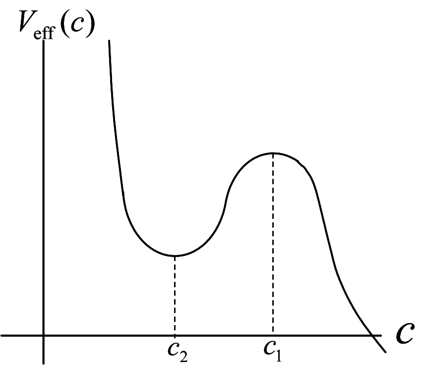
where the effective potential is defined as

A typical example of the effective potential is shown in Fig. 1. There are local minimum at $c=c_{2}$ and local maximum at $c=c_{1}$,respectively. One possible evolution is that from an unstable configuration to a stable one, namely from the solution of the radius $c_{1}$ to that of $c_{2}$. Assuming that correspondingly the brane curvature changes from $\lambda_{1}$ to $\lambda_{2}$ (We now allow for the possibility of $\lambda<0$), the flux conservation gives the relation

Noting that $c_{i}=\big(2\Lambda-2(D-1)\lambda_{i}/(D-2)\big)^{-1/2}$, the initial and final radii are related as

Clearly for $\lambda_{1}>\lambda_{\rm inst}$, $c_{2}<c_{1}$. Thus, we see that the radius of two-dimensional internal space must become smaller during the evolution, if the unstable configuration evolves to the stable one. There is other possibility of cosmological evolution: the decompactification $c\to\infty$, namely to the $(D+2)$-dimensional dS solution with expansion rate given by $(2\Lambda/D(D+1))^{1/2}$. These two possibilities may be distinguished in terms of the initial conditions. If initially $\dot{c}<0$ the radion evolves to the true minimum at $c=c_{2}$, whereas it may evolve to $c\to\infty$, if initially $\dot{c}>0$. We focus on more realistic the first possibility.

There is also another critical brane expansion rate

Note that always $\lambda_{\rm inst}<\lambda_{\rm AdS}<\lambda_{\rm max}$. For $\lambda_{\rm inst}<\lambda_{1}\leq\lambda_{\rm AdS}$, $\lambda_{2}\geq 0$ and thus the final $D$-dimensional geometry is dS, while for $\lambda_{\rm AdS}<\lambda_{1}<\lambda_{\rm max}$, $\lambda_{2}<0$ and the final stable $D$-dimensional geometry is anti- de Sitter (AdS). The thermodynamical arguments cannot be applied to AdS brane configurations since we should require the reality of the temperature $H^{D}$ (non-negativity of $\lambda$).

In Fig. 2, we showed a typical example of the magnetic flux as a function of $\lambda$. As is seen, for increasing $\lambda$, the flux takes a maximum value at $\lambda=\lambda_{\rm inst}$, then starts to decrease and vanishes at $\lambda_{\rm max}$. For the values of $\lambda_{\rm inst}<\lambda\leq\lambda_{\rm AdS}$, an unstable solution evolve to another dS configuration. For the $\lambda_{\rm AdS}<\lambda<\lambda_{\rm max}$, the corresponding stable configuration is AdS.

The above discussion can be naturally applied to more general cases $\alpha<1$. The observer on the (+)-brane cannot change the tension of (-)-brane and thus, $\phi/\beta_{-}$, i.e. $\tilde{\phi}$ defined in the previous subsection is conserved during the cosmological evolution. Oppositely for the observer on the (-)-brane and $\phi/\beta_{+}$ is conserved during the evolution. In the case $\alpha=1$, the critical expansion rate where dynamical instability appears is the exactly the point given by $(\partial\tilde{\phi}/\partial H^{D})_{\alpha}=0$. In general, since

$(\partial\tilde{\phi}/\partial H^{D})_{\eta}\neq(\partial\tilde{\phi}/\partial H^{D})_{\alpha}$. The special case is that of $\alpha=1$, where $\big(\partial\eta/\partial H^{D}\big)_{\alpha}\to 0$ and hence $(\partial\tilde{\phi}/\partial H^{D})_{\eta}=(\partial\tilde{\phi}/\partial H^{D})_{\alpha}$. The condition $(\partial\tilde{\phi}/\partial H^{D})_{\alpha}=0$ gives another curve on the $(\alpha,\lambda)$ plane as

Note that as special limits

and hence $\alpha\to 1$ $\lambda_{\rm inst}=\lambda_{\rm crit}=\lambda_{\ast}$ as we have seen previously. It supports that in the case $\alpha=1$, the cosmological evolution keeps the rugby ball shape during the cosmological evolution. However, in the cases $\alpha<1$, $\lambda_{\rm crit}\neq\lambda_{\ast}$ and hence it implies that the degree of warping $\alpha^{\prime}$ of the final stable configuration is different from that of the initial one $\alpha$ in general.

Before closing this section, in Fig. 3, we showed an example of $\lambda_{\rm max}$, $\lambda_{\rm crit}$ and $\lambda_{\ast}$ on the $(\alpha,\lambda)$ plane. As we see, in the limit $\alpha\to 1$, $\lambda_{\rm crit}$ and $\lambda_{\ast}$ coincide while in the opposite limit $\alpha\to 0$, $\lambda_{\ast}$ agrees with $\lambda_{\rm max}$. Thermodynamically unstable region corresponds to the region $\lambda_{\rm crit}<\lambda<\lambda_{\rm max}$ for each $\alpha$.

A class of six-dimensional Einstein-Maxwell-dilaton system has equivalent structure to the $(D+2)$-dimensional Einstein-Maxwell theory via dimensional reduction. We rewrite the $(D+2)$-dimensional metric as

where $(D-4)$-dimensional part is compactified and the field strength with ${}^{(D+2)}F_{ab}={}^{(D+2)}F_{ab}(x)\quad\text{and}\quad{}^{(D+2)}F_{mM}=0$. With the above ansatz, dimensional reduction on the $(D-4)$ -dimensional manifold yields

with identifications: Eq. (4),

and $F_{ab}:={}^{(D+2)}F_{ab}V_{D-4}^{1/2}$ ($V_{D-4}$ is the volume of the $(D-4)$-dimensional flat space). Here $F_{ab}$ denotes the electro-magnetic field strength. Again we set $M_{6}^{4}:=M_{D+2}^{D}V_{D-4}=1$, unless it should be shown explicitly. For $\gamma=1$ the action (43) coincides with the bosonic part of Nishino-Sezgin (Salam-Sezgin) supergravity (some fields are set to be zero consistently). From Eq. (4), $0\leq\gamma\leq 1$. After dimensional reduction, $D$ is a parameter related to the dilatonic coupling $\gamma$ as Eq. (4), and hence can be arbitrary real, non-negative number. In particular, Nishino-Sezgin supergravity ($\gamma=1$) [5] is reproduced by taking $D\to\infty$.

We also define the 3-brane tension as $\tau_{i}:=\sigma_{i}V_{D-4}$. The tension of the 3-brane does not couple to the dilatonic scalar field after dimensional reduction. According to the above-mentioned way, we derive the cosmological solutions in the six-dimensional theory Eq. (43) from the higher-dimensional dS brane solutions Eq. (2). We identify $e^{\phi}=\xi^{(1-\gamma^{2})/(1+\gamma^{2})}e^{Ht}$. Then the six-dimensional metric is found to be

where the proper time is defined by $\tau=\int e^{(D-4)Ht/4}dt$, and the scale factors $a(\tau):=e^{DHt/4}$ and $b(\tau):=e^{(D-4)Ht/4}$, respectively. We easily find that $a(\tau)\propto\tau^{1/\gamma^{2}}$ and $b(\tau)\propto\tau$, leading to an accelerating cosmological solution for $\gamma<1$. The case $\gamma=1$ is exactly the (extensions) scaling solution in supergravity [15, 16]. We also find $\varphi(\tau,\xi)=(2/\gamma)\ln b(\tau)+(2\gamma)/(1+\gamma^{2})\ln\xi$ and $F_{\xi\theta}=\big(\beta/\sqrt{2}\big)\big(Q/\xi^{2(2+\gamma^{2})/(1+\gamma^{2})}\big)$, respectively. Other than this simplest solution there are two analytically known cosmological solutions derived from Kasner-type generalizations of $(D+2)$ dimensional dS brane solutions, but in the later times both these two solutions approach the above simplest solution [16]. Hence the above power-law solution is the late time attractor.

As we mentioned in the previous section, the class of the Einstein-Maxwell-dilaton theory Eq. (43) has the equivalent structure to the higher-dimensional Einstein-Maxwell theory via dimensional reduction. A $(D+2)$-dimensional dS brane solution gives rise to the accelerating expanding cosmological solution. Thus, if a dS brane solution in $(D+2)$ dimensions is unstable, the corresponding cosmological solution given by Eq. (45) is also unstable. Since we assumed that the $D$-dimensional geometry keeps the Friedmann-Robertson-Walker form and hence there are no excitations of any perturbation mode which depends on the $(D-4)$-dimensional spatial dimensions, the smooth one-to-one correspondence of the $(D+2)$-dimensional Einstein-Maxwell theory with the six-dimensional Einstein-Maxwell-dilaton theory alway exists at all the times of cosmological evolutions. If there is a trajectory in the solution space in the $(D+2)$-dimensional theory, there also is a corresponding trajectory in the six-dimensional theory. It is also clear that the magnetic flux is conserved for the corresponding trajectory in six dimensions. The mass of an unstable mode scales as $M_{0}^{2}=\propto\mu_{0}^{2}/b(\tau)^{2}\propto\mu_{0}^{2}/\tau^{2}$ from the six dimensional point of view. If the final stable solution in $(D+2)$ dimensional theory is dS brane solution, then the corresponding cosmological solutions in six-dimensions is also a accelerating cosmological solution with smaller $\lambda$. If the final configuration in $(D+2)$-dimensions is AdS, then the corresponding six-dimensional solution would be a collapsing Universe, though there may be no analytic form since there is analytic description of AdS spacetime with the form of a flat Friedmann-Robertson-Walker metric.

The meaning of $\lambda$ for a four-dimensional observer becomes clearer from the perspectives of the four-dimensional effective theory. From the original $(D+2)$-dimensional metric

References

- [1] E. Papantonopoulos, arXiv:gr-qc/0601011.
- [2] J. W. Chen, M. A. Luty and E. Ponton, JHEP 0009, 012 (2000) [arXiv:hep-th/0003067]; S. M. Carroll and M. M. Guica, arXiv:hep-th/0302067; I. Navarro, JCAP 0309, 004 (2003) [arXiv:hep-th/0302129]; Y. Aghababaie, C. P. Burgess, S. L. Parameswaran and F. Quevedo, Nucl. Phys. B 680, 389 (2004) [arXiv:hep-th/0304256].
- [3] I. Navarro, Class. Quant. Grav. 20, 3603 (2003) [arXiv:hep-th/0305014]; H. P. Nilles, A. Papazoglou and G. Tasinato, Nucl. Phys. B 677, 405 (2004) [arXiv:hep-th/0309042]; H. M. Lee, Phys. Lett. B 587, 117 (2004) [arXiv:hep-th/0309050]; J. Vinet and J. M. Cline, Phys. Rev. D 70, 083514 (2004) [arXiv:hep-th/0406141]; J. Garriga and M. Porrati, JHEP 0408, 028 (2004) [arXiv:hep-th/0406158].
- [4] Y. Aghababaie et al., JHEP 0309, 037 (2003) [arXiv:hep-th/0308064]; G. W. Gibbons, R. Guven and C. N. Pope, Phys. Lett. B 595, 498 (2004) [arXiv:hep-th/0307238]; C. P. Burgess, F. Quevedo, G. Tasinato and I. Zavala, JHEP 0411, 069 (2004) [arXiv:hep-th/0408109].
- [5] H. Nishino and E. Sezgin, Phys. Lett. B 144, 187 (1984); A. Salam and E. Sezgin, Phys. Lett. B 147, 47 (1984); H. Nishino and E. Sezgin, Nucl. Phys. B 278, 353 (1986).
- [6] S. Mukohyama, Y. Sendouda, H. Yoshiguchi and S. Kinoshita, JCAP 0507, 013 (2005) [arXiv:hep-th/0506050];
- [7] J. M. Cline, J. Descheneau, M. Giovannini and J. Vinet, JHEP 0306, 048 (2003) [arXiv:hep-th/0304147].
- [8] I. Navarro and J. Santiago, JHEP 0502, 007 (2005) [arXiv:hep-th/0411250]; I. Navarro and J. Santiago, JCAP 0603, 015 (2006) [arXiv:hep-th/0505156].
- [9] M. Peloso, L. Sorbo and G. Tasinato, Phys. Rev. D 73, 104025 (2006) [arXiv:hep-th/0603026]; E. Papantonopoulos, A. Papazoglou and V. Zamarias, JHEP 0703, 002 (2007) [arXiv:hep-th/0611311]; T. Kobayashi and M. Minamitsuji, Phys. Rev. D 75, 104013 (2007) [arXiv:hep-th/0703029]; C. P. Burgess, D. Hoover and G. Tasinato, JHEP 0709, 124 (2007) [arXiv:0705.3212 [hep-th]].
- [10] J. Vinet and J. M. Cline, Phys. Rev. D 70, 083514 (2004) [arXiv:hep-th/0406141]; J. Vinet and J. M. Cline, Phys. Rev. D 71, 064011 (2005) [arXiv:hep-th/0501098].
- [11] E. Papantonopoulos, A. Papazoglou and V. Zamarias, arXiv:0707.1396 [hep-th]; M. Minamitsuji and D. Langlois, Phys. Rev. D 76, 084031 (2007) [arXiv:0707.1426 [hep-th]].
- [12] F. Chen, J. M. Cline and S. Kanno, arXiv:0801.0226 [hep-th].
- [13] S. Fujii, T. Kobayashi and T. Shiromizu, Phys. Rev. D 76, 104052 (2007) [arXiv:0708.2534 [hep-th]]; F. Arroja, T. Kobayashi, K. Koyama and T. Shiromizu, JCAP 0712, 006 (2007) [arXiv:0710.2539 [hep-th]].
- [14] B. Himmetoglu and M. Peloso, Nucl. Phys. B 773, 84 (2007) [arXiv:hep-th/0612140].
- [15] A. J. Tolley, C. P. Burgess, C. de Rham and D. Hoover, New J. Phys. 8, 324 (2006) [arXiv:hep-th/0608083]; E. J. Copeland and O. Seto, arXiv:0705.4169 [hep-th].
- [16] T. Kobayashi and M. Minamitsuji, JCAP 0707, 016 (2007) [arXiv:0705.3500 [hep-th]].
- [17] A. J. Tolley, C. P. Burgess, C. de Rham and D. Hoover, arXiv:0710.3769 [hep-th].
- [18] B. Cuadros-Melgar, E. Papantonopoulos, M. Tsoukalas and V. Zamarias, arXiv:0712.3232 [hep-th].
- [19] C. P. Burgess, C. de Rham, D. Hoover, D. Mason and A. J. Tolley, JCAP 0702, 009 (2007) [arXiv:hep-th/0610078]; H. M. Lee and A. Papazoglou, Nucl. Phys. B 747, 294 (2006) [Erratum-ibid. B 765, 200 (2007)] [arXiv:hep-th/0602208];
- [20] H. Yoshiguchi, S. Mukohyama, Y. Sendouda and S. Kinoshita, JCAP 0603, 018 (2006) [arXiv:hep-th/0512212]; Y. Sendouda, S. Kinoshita and S. Mukohyama, Class. Quant. Grav. 23, 7199 (2006) [arXiv:hep-th/0607189].
- [21] S. Kinoshita, Y. Sendouda and S. Mukohyama, JCAP 0705, 018 (2007) [arXiv:hep-th/0703271].
- [22] C. R. Contaldi, L. Kofman and M. Peloso, JCAP 0408, 007 (2004) [arXiv:hep-th/0403270].
- [23] O. DeWolfe, D. Z. Freedman, S. S. Gubser, G. T. Horowitz and I. Mitra, Phys. Rev. D 65, 064033 (2002) [arXiv:hep-th/0105047]; J. U. Martin, JCAP 0504, 010 (2005) [arXiv:hep-th/0412111].
- [24] P. G. O. Freund and M. A. Rubin, Phys. Lett. B 97, 233 (1980).
- [25] C. Krishnan, S. Paban and M. Zanic, JHEP 0505, 045 (2005) [arXiv:hep-th/0503025].
- [26] S. S. Gubser and I. Mitra, arXiv:hep-th/0009126; S. S. Gubser and I. Mitra, JHEP 0108, 018 (2001) [arXiv:hep-th/0011127].