Performance analysis of a cross-layer collaborative beamforming approach in the presence of channel and phase errors
Abstract
Collaborative beamforming enables nodes in a wireless network to transmit a common message over long distances in an energy efficient fashion. However, the process of making available the same message to all collaborating nodes introduces delays. The authors recently proposed a MAC-PHY cross-layer scheme that enables collaborative beamforming with significantly reduced collaboration overhead. The method requires knowledge of node locations and internode channel coefficients. In this paper, the performance of that approach is studied analytically in terms of average beampattern and symbol error probability (SEP) under realistic conditions, i.e., when imperfect channel estimates are used and when there are phase errors in the contributions of the collaborating nodes at the receiver.
Index Terms:
collaborative beamforming, cross-layer approach for wireless networks, imperfect conditionsI Introduction
Distributed, or collaborative, beamforming has been of considerable recent interest as a preferred solution for long-distance transmission in wireless networks, due to its energy efficiency [3],[4]. In conventional distributed beamforming schemes, a set of distributed nodes (called collaborating nodes) act as a virtual antenna array and form a beam to cooperatively transmit a common signal arising from a source node. Using knowledge of network coordinates, each collaborating node adjusts its initial phase so that the resulting beampattern focuses in the direction of the desired destination. The requirement that all collaborating nodes have access to the same message signal means that source nodes must share their message signals with collaborating nodes before beamforming. To study network performance, one must take into account the overhead (information-sharing time) required for node collaboration. If a time-division multiple-access (TDMA) scheme were to be employed, the information-sharing time would increase proportionally to the number of source nodes.
The authors recently proposed a MAC-PHY cross-layer technique in [2] and [5], based on the idea of collaborative beamforming of [4], to reduce the time required for information sharing and to allow simultaneous multiple beams. The main idea is as follows: for information-sharing, we consider a real physical model in which collaborating nodes receive linear mixtures of transmitted packets. Subsequently, each collaborating node transmits a weighted version of its received signal. The weights allow packets bound to the same destination to add coherently at the destination node. Each collaborating node computes its weight based on the estimated channel coefficients between sources and itself, and also based on estimates of node coordinates. In [2] and [5] the analysis was performed under the assumption that all required estimates are perfect. In this paper, we investigate performance under imperfect conditions, i.e., when there are channel estimation errors and phase errors.
II System model and proposed scheme
The notation used here is illustrated in Fig. 1. For simplicity, let us assume that sources and destinations are coplanar. The network is divided into clusters, so that nodes in a cluster can hear each other’s transmissions. During slot , source nodes in cluster tend to communicate with nodes that belong to clusters , respectively. The beamforming is performed by nodes in cluster . The collaborating nodes, designated as , are assumed to be uniformly distributed over a disk of radius . We denote the location of in polar coordinates with respect to the origin of the disk by . Let represent the distance between and the destination , and represent the distance between the origin of the disk and . If is the azimuthal angle of with respect to the origin of the disk, the polar coordinates of are . Moreover, let denote the distance between and some receiving point with polar coordinate .

We further make the following assumptions: (1) A slotted packet system is considered, in which each packet requires one slot for its transmission. Perfect synchronization is assumed between nodes in the same cluster. Nodes operate under half-duplex mode, i.e., they cannot receive while they are transmitting. (2) Nodes transmit packets consisting of phase-shift keying (PSK) symbols each having the same power . (3) Communication takes place over flat fading channels. The channel gain during slot between source and collaborating node is denoted by . For intra-cluster communications small-scale fading plays the dominant role. Thus, for a fixed , we model as circularly symmetric complex Gaussian random variables with zero means and variances (i.e., this is a Rayleigh fading model). The gains of different paths are assumed to be independent and identically distributed (i.i.d.). The gain of a given path is constant during the slot duration. (4) For inter-cluster communications, large-scale fading plays the dominant role. We assume that the distances between collaborating nodes and destinations are much greater than the maximum distance between source and collaborating nodes. Thus, the complex baseband-equivalent channel gain between nodes and during beamforming equals [7], where is the signal wavelength and is the path loss between the center of the disk containing the collaborating nodes and the destination.
In slot , all source nodes within the cluster simultaneously transmit their packets. The packet transmitted by node consists of symbols . Due to the broadcast nature of the wireless channel, non-active nodes in cluster hear a collision, i.e., a linear combination of the transmitted symbols. More specifically, node hears the signal
| (1) |
where represents noise at the receiving node . The noise is assumed to be zero-mean with covariance matrix , where denotes the identity matrix.
Suppose that in slot , the collaborating nodes need to beamform to destination . Each collaborating node transmits the signal
| (2) |
where is the initial phase of . is a scalar used to adjust the transmit power; it is the same for all collaborating nodes, and is on the order of .
Given the collaborating nodes at radial coordinates and azimuthal coordinates , the received signal at an arbitrary location with polar coordinates , is
| (3) |
where represents noise at the receiver during slot . The covariance matrix of equals .
The received signal at the destination during slot is
| (4) |
It was shown in [5] that, as and omitting the noise, . Thus, the destination node receives a scaled version of . The beamforming step is completed in slots, reinforcing one source signal at a time. Compared with the scheme in [4], the information sharing time is reduced from to 1. Multiple beams can be formed in one slot when source packets have distinct destinations. In the rest of the paper, for simplicity we will consider only the case in which a single beam is formed during slot , focusing on destination .
III Average Beampattern under Imperfect Conditions
The beampattern represents the distribution of received power along all azimuthal angles. We showed in [5] that, under perfect conditions the average beampattern is of a form similar to [4], with increased sidelobe level. In this section, we discuss effects of imperfect channels and phase on average beampattern, respectively.
III-A Imperfect Channels
We model as the imperfect estimate of , where is the estimation error. The estimation errors are i.i.d. Gaussian random variables, . The average beampattern with imperfect channels can be expressed as
| (5) |
where is the average beampattern related to perfect channels , and is the average beampattern related to the estimation error . Following steps similar to those leading to in [5], one can obtain
| (6) |
where represents the average SNR at the collaborating nodes. Note that is actually a constant independent of . In other words, the effect of imperfect channels on average beampattern is an increased sidelobe level.
III-B Imperfect Phase
Under imperfect phase, each collaborating node will transmit the signal , where the represents the phase error, which is assumed i.i.d. with respect to . We use the same model as in [4] for the phase errors. Regarding how to obtain the initial phase, two cases (closed-loop and open-loop) are considered (see [4] for details):
(1) For the closed-loop case, imperfect phase corresponds to the phase offset due to the phase ambiguity caused by carrier phase jitter or offset between the transmitter and receiver nodes. We assume that the phase error follows a Tikhonov distribution, which is a typical phase jitter model for phase-locked loop (PLL) circuits.
(2) For the open-loop case, imperfect phase results from estimation errors in the location parameters and . We assume the corresponding radius error is uniformly distributed over , and the angle error is uniformly distributed over . The radius and angle errors are further assumed to be mutually independent random variables, independent of and .
Based on the above phase error models, we can show that the expressions of the average beampattern are similar to the results in Section VI of [4] with the only difference being a scaling factor. Thus, as in [4], the basic effect of these phase errors is in reducing the power in the main lobe. The derivation is similar to that in [4] and is omitted here due to space limitations.
IV SEP under Imperfect Conditions
Under perfect conditions, the received signal (one sample) at the destination is given by
| (7) |
where . We showed in [2] that where .
Given , the instantaneous signal-to-interference-plus-noise ratio (SINR), , equals
| (8) |
where follows an Erlang distribution ().
IV-A Imperfect Channels
Taking channel errors into account, the received signal at the destination is given by
| (10) | |||||
Since the destination node does not have knowledge of , the term represents interference. Thus, in the interference term, and are coupled together, and the exact SEP would involve integration of all of the random variables ( and , ). In the sequel we will use an approximation that simplifies this analysis.
Let us define
| (11) |
It is easy to show that, given , and
| (12) |
According to the central limit theorem, when is large, is approximately normally distributed. Let us thus approximate the distribution of as . Taking into account the independence of and , the approximate instantaneous SINR, , equals
| (13) |
which contains only a single random variable . Finally, to calculate the SEP under imperfect channel conditions, let us substitute for in (9). The techniques in section IV-A of [2] can be used to obtain simple bounds for SEP.
IV-B Imperfect Phase
Imperfect phase has two effects on the receiver: signal power reduction and phase distortion [3]. Assuming that the phase distortion is compensated for by the coherent receiver (e.g., by pilots), here we focus on signal power reduction only.
We define the power reduction coefficient , where is the average received signal power with phase error and is the average signal power under perfect phase.
Taking phase errors into account, the received signal at the destination is given by
| (14) | |||||
where is the phase error of collaborating node .
Note that the statistics of are the same as those of ; so phase errors do not change the statistical behavior of the interference term.
Assuming we use a coherent receiver, the instantaneous SINR, , equals
| (15) |
Since and are coupled, the exact SEP includes integration with respect to and (), which is computationally complex. To facilitate analysis we make the following approximation for :
| (16) |
In other words, is approximated by the instantaneous SINR under perfect conditions scaled down by a coefficient .
It can be shown that
| (17) |
where depends on the specific phase error model used. Based on the phase error models in section III-B, has been derived in [4].
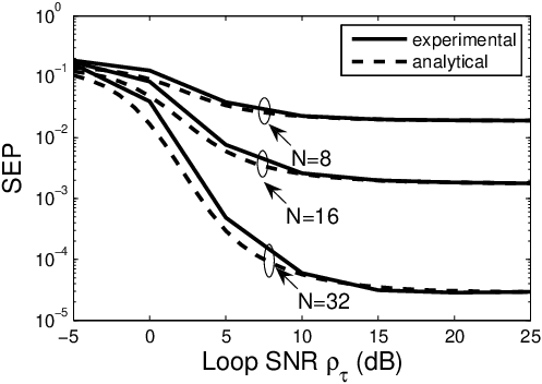
Simulation: In Fig. 3(a), we show the SEP as a function of loop SNR (closed-loop case). The variance of the phase error is . For the analytical SEP, we directly use the results in [4] to calculate and obtain in (17). As observed, dB may be necessary to achieve a satisfactory SEP. Fig. 3(b) shows the SEP vs. and (open-loop case), where both radius and angle errors are considered. One can see that the phase error in the open-loop case can severely degrade the SEP performance. Thus, it is important to investigate techniques that enable accurate location estimation. In both figures, the analytical result based on (16) match well the experimental results for a wide range of phase errors.
V conclusions
We have considered the cross-layer collaborative beamforming approach of [2] and [5], and we have analyzed its performance under imperfect conditions. For the average beampattern, the principal effect of imperfect channel information is increased sidelobe level, and the principal effect of imperfect phase information is reduced mainlobe power. We have provided approximate analytical expressions for the SEP under imperfect conditions, which show the effects of imperfect channel and phase on that quantity.
References
- [2] L. Dong, A. P. Petropulu and H. V. Poor, “Cooperative beamforming for wireless ad hoc networks,” in Proc. 2007 IEEE Global Commun. Conf., Washington, DC, Nov. 2007.
- [3] R. Mudumbai, G. Barriac and U. Madhow, “On the feasibility of distributed beamforming in wireless networks,” IEEE Trans. Wireless Commun, vol. 6, no. 5, pp. 1754-1763, May 2007.
- [4] H. Ochiai, P. Mitran, H. V. Poor and V. Tarokh, “Collaborative beamforming for distributed wireless ad hoc sensor networks,” IEEE Trans. Signal Process., vol. 53, no. 11, pp. 4110 - 4124, Nov. 2005.
- [5] A. P. Petropulu, L. Dong and H. V. Poor, “A high-throughput cross-layer scheme for distributed wireless ad hoc networks,” in Proc. 41st Conf. Inform. Sci. Syst., Baltimore, MD, Mar. 2007.
- [6] M. K. Simon and M.-S. Alouini, Digital Communication over Fading Channels (second edition). John Wiley & Sons, New York, 2005.
- [7] D. Tse and P. Viswanath, Fundamentals of Wireless Communication. Cambridge Univ Press, Cambridge, UK, 2005.

(a) closed-loop

(b) open-loop