跳到论文正文
W Papers独立论文阅读器 arXiv:0801.3038 论文正文 计算阅读时间 · 0%
引用这篇论文根据当前论文元数据生成,正式投稿前建议核对。


License: Assumed arXiv.org perpetual non-exclusive license
arXiv:0801.3038v1 [math.MG] 21 Jan 2008

Heat Kernels on Euclidean Complexes

Melanie Anne Pivarski
Abstract

In this thesis we describe a type of metric space called an Euclidean polyhedral complex. We define a Dirichlet form on it; this is used to give a corresponding heat kernel. We provide a uniform small time Poincaré inequality for complexes with bounded geometry and use this to determine uniform small time heat kernel bounds via a theorem of Sturm. We then consider such complexes with an underlying finitely generated group structure. We use techniques of Saloff-Coste and Pittet to show a large time asymptotic equivalence for the heat kernel on the complex and the heat kernel on the group.

\makecopyright{biosketch}

Melanie Pivarski was born on August 13, 1977 somewhere in the outskirts of Pittsburgh to Lynn and Thomas Pivarski. She grew up with her parents and two sisters, Kara and Janelle; her grandmother, Caroline Matovick, lived a few blocks away. They can all attest to the fact that yes, Melanie has always talked with her hands.

She attended Colfax Elementary School where she greatly enjoyed Ms. Kengor’s math classes; partly, this was because she could spend time doing logic puzzles. She was also involved in Girl Scouts with Chrissy. She then attended Springdale High School where she participated in many different activities, most notably art classes, Drama Club with Ms. Frauenholz, and Academic Games.

From 1995 through 1999, she attended Carnegie Mellon University, where she majored in mathematics and minored in computer science. While there, she took Prof. Mizel’s freshman analysis course out of Apostle. This class convinced her that she needed to study mathematics. In her analysis class she met Helena and Ruth who became her good friends and study partners. Computers are a part of the culture at CMU, and so she found herself in a number of fun computer science classes. Though she spent much of her time on math and computers, she found time to take some ballet classes with her friend Robert and some introductory Polish classes at the University of Pittsburgh. Quite significantly, she met Jim McCann (now Jim McCann Pivarski) during freshman orientation. They began dating that fall and were married in June of 1999.

Melanie and Jim moved to Ithaca in the summer of 1999, where they became graduate students in math and physics respectively. Melanie has greatly enjoyed her time in the math department; while there she was involved in the teaching seminars, the outreach program Expanding Your Horizons, the women in math potlucks, the 120A Cafe, and the Gingerbread House contests, specializing in tower constructions. She also studied some math.

Outside the math department, Melanie found many things to do. She’s taken ballet classes and sang in the choir at St. Catherine’s for much of her time here. She’s also been involved in the St Catherine’s young adult group, the PreCana team, and spent a few years helping out at Loaves and Fishes. Through all of this, she’s met a number of interesting people and had a variety of experiences. She considers herself to be more mature than she’s ever been before, and she hopes to continue growing and learning throughout her life.

In the fall of 2006, Melanie and Jim will move to College Station where they will be employed as postdocs at Texas A & M University. {dedication} To Friendship! And most especially to Jim!

Acknowledgements.
The math department at Cornell is full of wonderful people. The community here is splendiferous. I’m very grateful for the years spent here, the math learned, and especially the friendships. Most importantly, I’d like to thank my advisor, Prof. Saloff-Coste, who gave me an interesting problem to work on. He’s exposed me to loads of cool mathematics, and he has been essential in my learning some of it. He also has a nearly infinite amount of patience, which comes in quite handy. I’d also like to thank my committee members, Prof. Gross and Prof. Strichartz, who also helped me to develop mathematically through both courses and conversations. Thanks go to Prof. Fulling as well, who found a mistake in an early draft of this thesis. My mathematical siblings, David Revelle, Lee Gibson, Sharad Goel, Guan-Yu Chen, Evgueni Klebanov, Pavel Gyra, and Jessica Zuniga, are all great people. They’ve been very encouraging and quite helpful to me in clarifying my thoughts and definitions. I’ve learned a lot in our group meetings! Thanks go to Todd Kemp and Treven Wall, who helped me with various analysis bits, Jim Belk, who gave me a crash course in algebraic topology one summer, Kristin Camenga who helped me with the geometric definitions, and Mike Kozdron, who showed me to various latex commands. I’d also like to thank Josh Bowman, Jonathan Needleman, Robyn Miller, Mia Minnes, and Brigitta Vermesi who, along with many of the other folk mentioned above, helped me to organize my thoughts into some kind of presentable form through various conversations. Maria Belk and Maria Terrell should also be thanked for their encouragement and general good advice on how to be a graduate student.
\figurelistpage\symlist
  • •

    XX the complex

  • •

    X(k)X^{(k)} the kk-skeleton of XX

  • •

    γ\gamma a path in XX

  • •

    L⁡(γ)L(\gamma) length of γ\gamma

  • •

    dX​(⋅,⋅)d_{X}(\cdot,\cdot) distance in XX induced by the Euclidean metric

  • •

    dX(i)​(⋅,⋅)d_{X^{(i)}}(\cdot,\cdot), di​(⋅,⋅)d_{i}(\cdot,\cdot) distance in X(i)X^{(i)} induced by the Euclidean metric

  • •

    μ\mu measure on XX

  • •

    E⁡(⋅,⋅)E(\cdot,\cdot) energy form constructed via Γ\Gamma-limit

  • •

    ℰ⁡(⋅,⋅)\mathcal{E}(\cdot,\cdot) energy form constructed via gradients

  • •

    Δ\Delta, Δk\Delta^{k} Laplacian for XX, X(k)X^{(k)}

  • •

    ΔΩ\Delta^{\Omega} Laplacian for Ω⊂X\Omega\subset X with Dirichlet boundary condition

  • •

    ∇f\nabla f, FF gradient of ff

  • •

    d​μ​(x)d\mu(x), d​xdx equivalent ways of writing the differential form

  • •

    Lip⁡(X)\operatorname{Lip}(X) the set of Lipschitz functions on XX

  • •

    W1,p​(X)W^{1,p}(X) the Sobolev space on XX of functions in Lp​(X)L^{p}(X) with first derivatives in LpL^{p}

  • •

    C0Lip​(X)C_{0}^{\operatorname{Lip}}(X) the set of compactly supported Lipschitz functions on XX

  • •

    −∫B\mathchoice{{\vbox{\hbox{$\textstyle-$}}\kern-4.86108pt}}{{\vbox{\hbox{$\scriptstyle-$}}\kern-3.43057pt}}{{\vbox{\hbox{$\scriptscriptstyle-$}}\kern-2.908pt}}{{\vbox{\hbox{$\scriptscriptstyle-$}}\kern-2.76045pt}}\!\int_{B} average integral over the set BB

  • •

    IΩI_{\Omega} indicator function on Ω\Omega (1 if in Ω\Omega, 0 if not)

  • •

    fEf_{E} average value of ff on the set EE

  • •

    ∂E\partial E the boundary of the set EE

  • •

    S(k)S^{(k)} the kk-sphere

  • •

    WkW_{k}, Wj,kW_{j,k} wedges of a ball in XX

  • •

    N⁡(j)N(j) the list of indices of faces adjacent to WjW_{j} including jj

  • •

    MM degree bound on XX

  • •

    ℓ\ell lower bound on edge lengths of XX

  • •

    α\alpha smallest interior angle in XX

  • •

    κ\kappa constant related to multiples of radii

  • •

    R0R_{0} bound on radius defined in terms of κ\kappa

  • •

    CW​e​a​kC_{Weak} constant in weak Poincaré inequality

  • •

    CPC_{P} constant for the Poincaré inequality

  • •

    ℱ\mathcal{F} collection of balls in the Whitney cover

  • •

    rBr_{B} radius of the ball BB

  • •

    BzB_{z} the central ball in the Whitney cover

  • •

    ℱ⁡(B)\mathcal{F}(B) a string of balls that takes BzB_{z} to BB

  • •

    ht​(x,y)h_{t}(x,y), htk​(x,y)h^{k}_{t}(x,y) heat kernel on XX, X(k)X^{(k)}

  • •

    HtH_{t} heat semigroup on XX

  • •

    τ\tau exit time for Brownian motion on a set

  • •

    XtX_{t} random variable for location of a Brownian motion in a subset of XX

  • •

    htΩ​(x,y)h^{\Omega}_{t}(x,y) heat kernel on Ω⊂X\Omega\subset X

  • •

    HtΩH_{t}^{\Omega} heat semigroup on Ω⊂X\Omega\subset X

  • •

    pt​(x,y)p_{t}(x,y), ptA​(x,y)p_{t}^{A}(x,y) heat kernel on GG, A⊂GA\subset G

  • •

    KnK^{n}, KAnK^{n}_{A} nn step transition operator on GG, A⊂GA\subset G

  • •

    λΩ​(i)\lambda_{\Omega}(i) ith eigenvalue for H1ΩH_{1}^{\Omega}

  • •

    βA​(i)\beta_{A}(i) ith eigenvalue for KA1K^{1}_{A}

  • •

    Tr⁡(Kn)\operatorname{Tr}{(K^{n})} trace of KnK^{n}

  • •

    GG group

  • •

    SS generating set for GG

  • •

    YY compact subset of XX with the property X/Y=GX/Y=G

  • •

    |g||g| word length of g∈Gg\in G

  • •

    dG​(⋅,⋅)d_{G}(\cdot,\cdot) distance in GG with respect to word length

  • •

    dY​(⋅,⋅)d_{Y}(\cdot,\cdot) distance in YY based on Euclidean paths in YY.

  • •

    diam⁡(Y)\operatorname{diam}(Y) diameter of YY with respect to dYd_{Y}

  • •

    Y(i)Y^{(i)} the ii skeleton of YY; X(i)∩YX^{(i)}\cap Y

  • •

    |A||A|, #​A\#A number of elements in AA

  • •

    Vol\operatorname{Vol}, VolX\operatorname{Vol}_{X}, VolG\operatorname{Vol}_{G} volume (with respect to XX, GG)

  • •

    BrB_{r}, BX​(r)B_{X}(r), BG​(r)B_{G}(r) ball of radius rr (in XX, GG)

  • •

    BX​(x,r)B_{X}(x,r), BG​(g,r)B_{G}(g,r) ball in XX (GG) with radius rr centered at xx (gg)

  • •

    E⁡(f,f)E(f,f) energy form; for GG this is 1|S|​∑g∈G∑s∈S|f⁡(g)−f⁡(g​s)|2\frac{1}{|S|}\sum_{g\in G}\sum_{s\in S}|f(g)-f(gs)|^{2}, for XX this is −⟨∇f,∇f⟩-\langle\nabla f,\nabla f\rangle

  • •

    |∇f​(x)||\nabla f(x)| length of gradient; on GG this is 1|S|​∑s∈S|f⁡(x)−f⁡(x​s)|2\sqrt{\frac{1}{|S|}\sum_{s\in S}|f(x)-f(xs)|^{2}}.

  • •

    ‖f‖p,A||f||_{p,A} the LpL^{p} norm restricted to a subset AA; for GG this is (∑x∈A|f⁡(x)|p)1/p(\sum_{x\in A}|f(x)|^{p})^{1/p}, for XX this is (∫A|f⁡(x)|p​𝑑x)1/p(\int_{A}|f(x)|^{p}dx)^{1/p}

  • •

    {γi}i=1N\{\gamma_{i}\}_{i=1}^{N} centers of the balls of radius δ\delta covering YY

  • •

    {gγi}i=1..N;g∈G\{g\gamma_{i}\}_{i=1..N;g\in G} centers of the balls of radius δ\delta covering XX

  • •

    CN,SC_{N,S} maximum number of balls overlapping a point in XX

  • •

    group⁡f\operatorname{group}f a new function from (G,N)→R(G,N)\rightarrow R defined to be −∫BX​(g​γi,δ)f(x)dx\mathchoice{{\vbox{\hbox{$\textstyle-$}}\kern-4.86108pt}}{{\vbox{\hbox{$\scriptstyle-$}}\kern-3.43057pt}}{{\vbox{\hbox{$\scriptscriptstyle-$}}\kern-2.908pt}}{{\vbox{\hbox{$\scriptscriptstyle-$}}\kern-2.76045pt}}\!\int_{B_{X}(g\gamma_{i},\delta)}f(x)dx

  • •

    CX​GC_{XG}, C0C_{0} constants used to compare metrics in GG and XX

  • •

    CHC_{H} constant for the Harnack inequality

  • •

    χ\chi, χg\chi_{g} a smooth function on XX, χ\chi translated by gg

  • •

    Cs​u​pC_{sup} constant used to bound the support of χ\chi

  • •

    CO​v​e​rC_{Over} constant bound on the maximum number of χg\chi_{g} supported at any point in X

  • •

    CgC_{g} bound on the magnitude of the gradient of χ\chi

  • •

    comp⁡f⁡(x)\operatorname{comp}f(x) a new function from X→RX\rightarrow R defined by ∑g∈Gf⁡(g)​χg​(x)\sum_{g\in G}f(g)\chi_{g}(x)

  • •

    Cg​r​a​dC_{grad} constant bound comparing norms of gradients

  • •

    ⌊x⌋\lfloor x\rfloor the largest integer less than or equal to xx

  • •

    ⌈x⌉\lceil x\rceil the smallest integer greater than or equal to xx

  • •

    C0​(Ω)C_{0}(\Omega) continuous funcions which are compactly supported in Ω\Omega

  • •

    U⁡(A)U(A) subset of XX depending on AA

\normalspacing

Chapter 1 Setup for the Complexes

1.1 Introduction

We will study how local and global geometries affect heat kernels on a set of metric spaces called Euclidean polyhedral complexes.

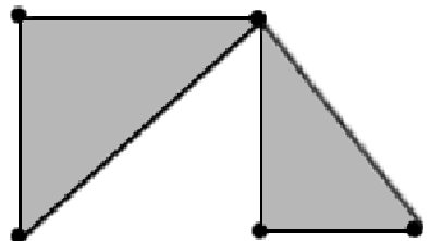
Euclidean complexes are formed by taking a collection of nn dimensional convex polytopes and joining them along n−1n-1 dimensional faces. Within each polytope, we will have the same metric structure as RnR^{n}. When we join them, we will glue the faces of two polytopes together so that points on one face are identified with points on the other face, and the metrics on those faces are preserved. We will require that these structures have a countable number of polytopes, are locally finite, and have lower bound on the interior angles and edge lengths. The complex formed by looking at kk dimensional faces is called the kk-skeleton. For instance, the 0-skeleton is set of vertices. A 1-skeleton is a graph where the space includes both vertices and points on the edges; sometimes this is called a metric graph [24]. Note that we can triangulate any convex polytope to obtain a collection of simplices, and so this structure is essentially equivalent to looking at a simplicial complex.

Refer to caption
Refer to caption
Refer to caption
Figure 1.1: Example of a 2 dimensional Euclidean Complex (left), its 1-skeleton (center), one possible triangulation (right).

Let htk​(x,y)h_{t}^{k}(x,y) be the heat kernel on the kk-skeleton. This is the fundamental solution to the heat equation ∂tu−Δ​u=0\partial_{t}u-\Delta u=0 on the kk-skeleton. It can be used to describe the probability that we travel from xx to yy in time tt when our movement is restricted to the kk-skeleton.

Theorem 1.1.1.

For XX a uniformly locally finite Euclidean complex of dimension nn whose interior angles and edge lengths are bounded below. Fix T∈(0,∞)T\in(0,\infty). There exist c,C∈(0,∞)c,C\in(0,\infty) such that for any x∈Xx\in X and t<Tt<T we have:

ctk/2≤htk​(x,x)≤Ctk/2.\displaystyle\frac{c}{t^{k/2}}\leq h_{t}^{k}(x,x)\leq\frac{C}{t^{k/2}}.

Note that this claims that the heat kernel on the kk-skeleton behaves, up to a constant that is independent of where in XX we are, like the heat kernel on RkR^{k} asymptotically when t→0t\rightarrow 0. The local behavior reflects the local geometry and structure of our space.

Theorems in Sturm [30] can be applied to Euclidean complexes to show that on any compact subset of X(k)X^{(k)}, the heat kernel is locally like the one on RkR^{k}, with constants that depend on the choice of compact subset. The essential difference in our theorem is that the constants are uniform throughout the entire complex.

An interesting example of these complexes comes from biology. In a paper by Billera, Holmes, and Vogtmann [3] they describe a way of classifying distances between phylogenetic trees, which are trees that describe evolution of species. One can form an Euclidean complex, where each of the faces corresponds to a different tree, and one moves through the points in the face by changing the edge lengths in the tree. One can then consider probability distributions on this space to determine likely genetic ancestry.

Euclidean complexes are also examples of fractal “blow-ups”, which are infinite fractals that are locally nice but globally have a structure with repetition. See Kigami [22] for a description of these fractals. In this setting, our small time asymptotic estimates apply. Note that these examples need not be compact. In [1], Barlow and Kumagai studied the small time asymptotic of heat kernels for compact self-similar sets.

Another collection of examples can be found by considering metric spaces, XX, which are acted upon by a finitely generated group, GG of isometries. When we take the space and mod out by that group, we obtain a compact set Y=X/GY=X/G. When YY can be expressed as a finite Euclidean complex, then XX is an Euclidean complex as well. Note that the kk-skeleton of YY will be the (kCLOSE(k-skeleton of OPENX)/GX)/G. A simple example of this is X=R2X=\mbox{\bf R}^{2}, Y=Y= the unit square, and G=Z2G=\mbox{\bf Z}^{2}. A more interesting example occurs when GG is the free group; there the space is globally hyperbolic, but locally Euclidean. With this added group structure, we can describe the large time behavior of the heat kernel. We write the heat kernel on a group as pt​(⋅,⋅)p_{t}(\cdot,\cdot).

Proposition 1.1.2.

Let XX be a locally finite countable Euclidean complex of dimension nn and let GG be finitely generated group GG. If X/GX/G is a complex comprised of a finite number of polytopes with Euclidean metric, we have:

pt​(x,x)≃ht​(x,x)​ as ​t→∞.\displaystyle p_{t}(x,x)\simeq h_{t}(x,x)\mbox{ as }t\rightarrow\infty.

Our main result says that, up to a constant, the heat kernel will behave the same asymptotically as t→∞t\rightarrow\infty on both the group and the complex. By transitivity, it will behave the same asymptotically regardless of which kk-skeleton we consider.

This theorem relates to a paper of Pittet and Saloff-Coste [26]. They show that a manifold MM which has a finitely generated group of isometries GG satisfies s​u​px​htM​(x,x)≃htG​(e,e)sup_{x}h^{M}_{t}(x,x)\simeq h^{G}_{t}(e,e) for large tt.

In chapter one, we describe our set-up. We provide definitions for the complex and skeletons and then define an energy form and a Laplacian on them. In chapter two, we will prove the initial theorem by first showing that a series of Poincaré inequalities hold, starting with one for balls where the radius of the ball depends on the center and generalizing until the result is uniform in space. In chapter three, we apply these inequalities to a result of Sturm [29] to yield a small time on diagonal heat kernel asymptotic with a uniform constant. We also provide off diagonal estimates with constants that depend on d⁡(x,y)d(x,y), but not on where xx and yy are located. We give several examples of heat kernels. In chapter four, we consider complexes with underlying group structure. We describe how to compare metrics on the complex and those on the underlying group, as well as how to switch from a function on a group to one on a complex and vice versa. We then use the metric comparison as well as our small time Poincaré inequality to compare norms of functions on complexes and their group counterparts. In chapter five, we consider heat kernels on the group and the complex. We split into two cases; nonamenable groups, which have exponentially fast heat kernel decay, and amenable groups. For the amenable groups, we look at heat kernels restricted to subsets of our space, and then take a Følner sequence to limit to a bound on the heat kernels themselves. In this way, we prove the second theorem.

1.2 Geometry of the Complexes

We will take our definitions of polytopes and polyhedral sets from Grünbaum’s Convex Polytopes [16].

Definition 1.2.1.

A polyhedron KK is a subset of RnR^{n} formed by intersecting a finite family of closed half spaces of RnR^{n}. Note that this can be an unbounded set, but it will be convex.

Definition 1.2.2.

A set FF is a face of KK if F=∅F=\emptyset, F=KF=K, or if F=H∩KF=H\cap K where HH is a supporting hyperplane of KK. HH is a supporting hyperplane of KK if H∩K≠∅H\cap K\neq\emptyset and HH does not cut KK into two pieces.

Definition 1.2.3.

A point x∈Kx\in K is an extreme point of a set KK if the only y,z∈Ky,z\in K which are solutions to x=λ​y+(1−λ)​zx=\lambda y+(1-\lambda)z for some λ∈(0,1)\lambda\in(0,1) are x=y=zx=y=z. That is, xx cannot be expressed as a convex combination of points in K−{x}K-\{x\}. Note that the extreme points of KK are faces for KK.

Definition 1.2.4.

A polytope is a compact convex subset of RnR^{n} which has a finite set of extreme points. This is equivalent to saying it is a bounded polyhedron.

Definition 1.2.5.

A polyhedral complex XX is the union of a collection, 𝒳\mathcal{X}, of convex polyhedra which are joined along lower dimensional faces. By this we mean that for any two distinct polyhedra P1,P2∈𝒳P_{1},P_{2}\in\mathcal{X},

  • •

    P1∩P2P_{1}\cap P_{2} is a polyhedron whose dimension satisfies
    dim(P1∩P2)<max⁡(dim(P1),dim(P2))\dim(P_{1}\cap P_{2})<\max(\dim(P_{1}),\dim(P_{2})) and

  • •

    P1∩P2P_{1}\cap P_{2} is a face of both P1P_{1} and P2P_{2}. We allow this face to be the empty set.

We do not have a specific embedding for the complex, XX; however, we require each polyhedra to have a metric which is consistent with that of its faces.

Note that this definition implied P1∩P2P_{1}\cap P_{2} is a connected set. This rules out expressing a circle as two edges whose ends are joined, but it allows us to write it as a triangle of three edges. This is not very restrictive, as we can triangulate the polyhedra in order to form a complex which avoids the overlap.

Simplicial complexes are an example of a polyhedral complex; the difference here is that we allow greater numbers of sides. Note that we allow infinite polyhedra, not just finite polytopes.

Definition 1.2.6.

Define a pp-skeleton, X(p)X^{(p)}, for 0≤p≤dimX0\leq p\leq\dim X to be the union of all faces of dimension pp or smaller. Note that this is also a polyhedral complex.

Definition 1.2.7.

A maximal polyhedron is a polyhedron that is not a proper face of any other polyhedron. The set of maximal polyhedra of XX is denoted 𝒳M​A​X\mathcal{X}_{MAX}. We say XX is dimensionally homogeneous if all of its maximal polyhedra have dimension nn. Note that in combinatorics literature this is called pure.

Definition 1.2.8.

XX is locally (n-1)-chainable if for every connected open set U⊂XU\subset X, U−X(n−2)U-X^{(n-2)} is also connected. For a dimensionally homogeneous complex XX this is equivalent to the property that any two nn dimensional polyhedra that share a lower dimensional face can be joined by a chain of contiguous (n−1)(n-1) or nn dimensional polyhedra containing that face.

Definition 1.2.9.

We call XX admissible if it is both dimensionally homogeneous and in some triangulation XX is locally (n-1)-chainable.

Refer to caption
Refer to caption
Refer to caption
Figure 1.2: Examples of a complex which is not dimensionally homogeneous (left), one which is not 1-chainable (center), and one which is admissible (right).

We will be working with connected admissible complexes, and for our purposes, we’d like to consider polyhedra that have an Euclidean metric. Let XX be an n-dimensional complex. When two polyhedra share a face, we require these metrics to coincide. For points xx and yy in different polyhedra, we define the distance as follows.

Definition 1.2.10.

Consider the set of paths connecting xx to yy which consist of a finite number of line segments. We can label each of these by the points it crosses in the (n−1)(n-1) skeleton. Set γ={x=x0,x1,x2,..,xk=y}\gamma=\{x=x_{0},x_{1},x_{2},..,x_{k}=y\} where xi∈x_{i}\in (n−1)(n-1)-skeleton for i=1..k−1i=1..k-1, and xix_{i}, xi+1x_{i+1} are both in the closure of the same maximal polyhedron. Then set L⁡(γ)=∑i=1kd⁡(xi−1,xi)L(\gamma)=\sum_{i=1}^{k}d(x_{i-1},x_{i}). We define the distance between points in different polyhedra to be d⁡(x,y)=infγL⁡(γ)d(x,y)=\inf_{\gamma}L(\gamma).

Essentially, we are splitting the path into pieces, and letting the lengths of those pieces inside of the simplices be the standard lengths in RnR^{n}. Since our complex is created using closed polyhedra, if the geometry of the polyhedra is bounded, the inf will be realized. This will give us a length space; ie, one in which distances are realized by geodesics in the space. Discussions of length spaces and other metric measure spaces can be found in Heinonen [18] and Burago, Burago, and Ivanov [6].

Definition 1.2.11.

Let X=∪iPiX=\cup_{i}P_{i}, where the PiP_{i} are the maximal polyhedra. We will set the measure of AA, a Borel subset of XX, to be μ⁡(A)=∑iμi​(A∩Pi)\mu(A)=\sum_{i}\mu_{i}(A\cap P_{i}) where μi\mu_{i} is the Lebesgue measure on PiP_{i}.

Notice that the measure within the interior of maximal polyhedra is the same as Lebesgue measure on RnR^{n}. This means that locally we will have all of the structure of RnR^{n}; in particular, we will have volume doubling for balls contained in the interior of the maximal polyhedra. Since our complex is locally finite, volume doubling will hold locally for all points in the complex.

Definition 1.2.12.

An admissible polyhedral complex, XX, equipped with distance, d⁡(⋅,⋅)d(\cdot,\cdot) and measure μ\mu is called an Euclidean polyhedral complex.

For brevity, we will often call this an Euclidean complex. A book which describes these complexes is Harmonic Maps Between Riemannian Polyhedra [11]. In it, the authors define these structures with a Riemannian metric and provide analytic results on both the complexes and functions whose domain and range are both complexes.

1.3 Analysis on the Complexes

1.3.1 The Dirichlet Form

Now that we’ve defined the space geometrically, we will define a Dirichlet form whose core consists of compactly supported Lipschitz functions.

Definition 1.3.1.

A function ff on a metric space XX is called LL-Lipschitz (alternately, Lipschitz) if there exists a constant L≥0L\geq 0 so that d⁡(f⁡(x),f⁡(y))≤L​dX​(x,y)d(f(x),f(y))\leq Ld_{X}(x,y) for all xx and yy in XX. The space of Lipschitz functions is denoted Lip⁡(X)\operatorname{Lip}(X). The space of compactly supported Lipschitz functions is denoted C0Lip​(X)C_{0}^{\operatorname{Lip}}(X).

Note that Lipschitz functions are continuous. By theorem 4 in section 5.8 of [12], for each Bϵ​(x)⊂X−X(n−1)B_{\epsilon}(x)\subset X-X^{(n-1)} and f∈C0Lip​(X)f\in C_{0}^{\operatorname{Lip}}\left(X\right), ff restricted to Bϵ​(x)B_{\epsilon}(x) is in the Sobolev space W1,∞​(Bϵ​(x))W^{1,\infty}\left(B_{\epsilon}(x)\right). This tells us that ff has a gradient almost everywhere in X−X(n−1)X-X^{(n-1)}. Since μ⁡(X(n−1))=0\mu(X^{(n-1)})=0, ff has a gradient for almost every xx in XX.

We would like an energy form that acts like E⁡(u,v)=∫X⟨∇u,∇v⟩​𝑑μE(u,v)=\int_{X}\langle\nabla u,\nabla v\rangle d\mu with domain FF to define our operator Δ\Delta with domain Dom⁡(Δ)\operatorname{Dom}(\Delta). We can define this in a very general manner which does not depend on the local Euclidean structure by following a paper of Sturm [31]. We can also define it in a more straightforward manner which uses the geometry of XX. We do both, and then show that they coincide.

Sturm assumes that the space (X,d)(X,d) is a locally compact separable metric space, μ\mu is a Radon measure on XX, and that μ⁡(U)>0\mu(U)>0 for every nonempty open set U⊂XU\subset X. These assumptions hold both in our space, XX, and on the skeletons, X(k)X^{(k)}. We begin by approximating EE with a form ErE^{r} defined to be:

Er​(u,v):=∫X∫B⁡(x,r)−{x}(u⁡(x)−u⁡(y))​(v⁡(x)−v⁡(y))d2​(x,y)​2​N​d​μ​(y)​d​μ​(x)μ⁡(Br​(x))+μ⁡(Br​(y))\displaystyle E^{r}(u,v):=\int_{X}\int_{B(x,r)-\{x\}}\frac{(u(x)-u(y))(v(x)-v(y))}{d^{2}(x,y)}\frac{2Nd\mu(y)d\mu(x)}{\mu(B_{r}(x))+\mu(B_{r}(y))}

for u,v∈Lip⁡(X)u,v\in\operatorname{Lip}(X) where N is the local dimension. Note that whenever xx is in a region locally like RnR^{n}, we have

limr→0Nμ​(Br​(x))​∫B⁡(x,r)−{x}(u⁡(x)−u⁡(y))2d2​(x,y)​𝑑μ​(y)=|∇u​(x)|2,\displaystyle\mathop{\lim}_{r\rightarrow 0}\frac{N}{\mu(B_{r}(x))}\int_{B(x,r)-\{x\}}\frac{(u(x)-u(y))^{2}}{d^{2}(x,y)}d\mu(y)=|\nabla u(x)|^{2},

and so this form looks very similar to E⁡(u,u)=∫X|∇u|2​𝑑xE(u,u)=\int_{X}|\nabla u|^{2}dx.

This form with domain C0Lip​(X)C_{0}^{\operatorname{Lip}}(X) is closable and symmetric on L2​(X)L^{2}(X), and its closure has core C0Lip​(X)C_{0}^{\operatorname{Lip}}(X). See Lemma 3.1 in [31]. One can take limits of these operators in the following way. The Γ\Gamma-limit of the ErnE^{r_{n}} is defined to be the limit that occurs when the following lim sup and lim inf are equal for all u∈L2​(X,m)u\in L^{2}(X,m). See Dal Maso[9] for a thorough introduction.

Γ−limsupn→∞⁡Ern​(u,u)\displaystyle\Gamma-\mathop{\lim\sup}_{n\rightarrow\infty}E^{r_{n}}(u,u) :=limα→0limsupn→∞⁡infv∈L2​(X)‖u−v‖≤αErn​(v,v)\displaystyle:=\mathop{\lim}_{\alpha\rightarrow 0}\mathop{\lim\sup}_{n\rightarrow\infty}\mathop{\mathop{\inf}_{v\in L^{2}(X)}}_{||u-v||\leq\alpha}E^{r_{n}}(v,v)
Γ−liminfn→∞⁡Ern​(u,u)\displaystyle\Gamma-\mathop{\lim\inf}_{n\rightarrow\infty}E^{r_{n}}(u,u) :=limα→0liminfn→∞⁡infv∈L2​(X)‖u−v‖≤αErn​(v,v).\displaystyle:=\mathop{\lim}_{\alpha\rightarrow 0}\mathop{\lim\inf}_{n\rightarrow\infty}\mathop{\mathop{\inf}_{v\in L^{2}(X)}}_{||u-v||\leq\alpha}E^{r_{n}}(v,v).

For any sequence {Ern}\{E^{r_{n}}\} of these operators with rn→0r_{n}\rightarrow 0 , there is a subsequence {rn′}\{r_{n^{\prime}}\} so that the Γ\Gamma-limit of Ern′E^{r_{n}^{\prime}} exists by Lemma 4.4 in [31]. These lemmas are put together into a theorem (5.5 in [31]) that tells us that this limit, E0E^{0}, with domain C0Lip​(X)C_{0}^{\operatorname{Lip}}(X) is a closable and symmetric form, and its closure, (E,F)(E,F), is a strongly local regular Dirichlet form on L2​(X,m)L^{2}(X,m) with core C0Lip​(X)C_{0}^{\operatorname{Lip}}(X).

Alternately, we can define the energy form using the structure of the space. We set ℰ⁡(⋅,⋅)\mathcal{E}(\cdot,\cdot) to the following for f∈C0Lip​(X)f\in C_{0}^{\operatorname{Lip}}(X):

ℰ⁡(f,f)=∑XM∈ℳ∫XM|∇f|2​𝑑μ​(x).\displaystyle\mathcal{E}(f,f)=\sum_{X_{M}\in\mathcal{M}}\int_{X_{M}}|\nabla f|^{2}d\mu(x).
Lemma 1.3.2.

ℰ⁡(⋅,⋅)\mathcal{E}(\cdot,\cdot) is a closable form. That is, for any sequence
{fn}n=1∞⊂C0Lip​(X)\{f_{n}\}_{n=1}^{\infty}\subset C_{0}^{\operatorname{Lip}}\left(X\right) that converges to 0 in L2​(X)L^{2}(X) and is Cauchy in ||⋅||2+ℰ(⋅,⋅)||\cdot||_{2}+\mathcal{E}(\cdot,\cdot) we have limn→∞ℰ⁡(fn,fn)=0\lim_{n\rightarrow\infty}\mathcal{E}(f_{n},f_{n})=0.

Proof.

To show this, we will first look at what happens on one fixed polyhedron, and then look at what happens on a complex. Let XMX_{M} be a maximal polyhedron. Since {fn}n=1∞\{f_{n}\}_{n=1}^{\infty} is Cauchy in the norm, we have

limm,n→∞(∫XM(fn−fm)2​𝑑μ)12+(∫XM(∇fn−∇fm)2​𝑑μ)12=0.\displaystyle\lim_{m,n\rightarrow\infty}\left(\int_{X_{M}}(f_{n}-f_{m})^{2}d\mu\right)^{\frac{1}{2}}+\left(\int_{X_{M}}(\nabla f_{n}-\nabla f_{m})^{2}d\mu\right)^{\frac{1}{2}}=0.

This gives us two functions, ff and FF which are the limits of fnf_{n} and ∇fn\nabla f_{n} respectively. We have f=0f=0 by assumption. We need to show that F=0F=0. For almost every x,y∈XMx,y\in X_{M} and line γx∼y\gamma_{x\sim y} in XMX_{M} we have

∫γx∼y∇fn​𝑑μ=fn​(y)−fn​(x).\displaystyle\int_{\gamma_{x\sim y}}\nabla f_{n}d\mu=f_{n}(y)-f_{n}(x).

Then we can take the limit as nn goes to infinity to get

limn→∞∫γx∼y∇fn​𝑑μ=limn→∞fn​(y)−fn​(x)=0.\displaystyle\lim_{n\rightarrow\infty}\int_{\gamma_{x\sim y}}\nabla f_{n}d\mu=\lim_{n\rightarrow\infty}f_{n}(y)-f_{n}(x)=0.

This gives us limn→∞∇fn​(x)=0\lim_{n\rightarrow\infty}\nabla f_{n}(x)=0 for almost every x∈XMx\in X_{M}.

Since the choice of XMX_{M} was arbitrary, this shows limn→∞∇fn​(x)=0\lim_{n\rightarrow\infty}\nabla f_{n}(x)=0 for almost every x∈Xx\in X.

Showing L2L^{2} convergence is a bit trickier, as we need to show that we can interchange the limit with the sum over the maximal polyhedra. We can do this for |∇fn−∇fm||\nabla f_{n}-\nabla f_{m}| by Fatou’s Lemma.

limn→∞∑XM∈ℳ∫XM|∇fn|2​𝑑μ\displaystyle\lim_{n\rightarrow\infty}\sum_{X_{M}\in\mathcal{M}}\int_{X_{M}}|\nabla f_{n}|^{2}d\mu =\displaystyle= limn→∞∑XM∈ℳ∫XM|∇fn−limm→∞∇fm|2​𝑑μ\displaystyle\lim_{n\rightarrow\infty}\sum_{X_{M}\in\mathcal{M}}\int_{X_{M}}|\nabla f_{n}-\lim_{m\rightarrow\infty}\nabla f_{m}|^{2}d\mu
=\displaystyle= limn→∞∑XM∈ℳ∫XMlimm→∞|∇fn−∇fm|2​𝑑μ\displaystyle\lim_{n\rightarrow\infty}\sum_{X_{M}\in\mathcal{M}}\int_{X_{M}}\lim_{m\rightarrow\infty}|\nabla f_{n}-\nabla f_{m}|^{2}d\mu
≤\displaystyle\leq limn→∞limm→∞∑XM∈ℳ∫XM|∇fn−∇fm|2​𝑑μ\displaystyle\lim_{n\rightarrow\infty}\lim_{m\rightarrow\infty}\sum_{X_{M}\in\mathcal{M}}\int_{X_{M}}|\nabla f_{n}-\nabla f_{m}|^{2}d\mu
=\displaystyle= 0.\displaystyle 0.

This tells us that the form is closable. ∎

We will show that the two energy forms are the same. To do this, we show that they are the same on the core C0Lip​(X)C_{0}^{\operatorname{Lip}}\left(X\right); this gives equality on the domain.

Lemma 1.3.3.

Each function f∈C0Lip​(X)f\in C_{0}^{\operatorname{Lip}}\left(X\right) satisfies E⁡(f,f)=ℰ⁡(f,f)E(f,f)=\mathcal{E}(f,f).

Proof.

We can write XX as (X−X(n−1))∪X(n−1)(X-X^{(n-1)})\cup X^{(n-1)}; this is a collection of maximal polyhedra and a set of measure 0. The interior of the maximal polyhedra is a Riemannian manifold without boundary. XX is also a locally compact length space, and so it satisfies the conditions of example 4G in [30]. This implies it has the strong measure contraction property with an exceptional set. Corollary 5.7 in [30] says that this then has E⁡(f,f)=ℰ⁡(f,f)E(f,f)=\mathcal{E}(f,f) for each f∈C0Lip​(X)f\in C_{0}^{\operatorname{Lip}}(X). The equality is shown by approximating the forms using an increasing sequence of open subsets which limit to X−X(n−1)X-X^{(n-1)}. As C0Lip​(X)C_{0}^{\operatorname{Lip}}(X) is a core for both EE and ℰ\mathcal{E}, the Dirichlet forms are the same. ∎

We will explain more clearly where the domain of this operator lies. The domain is the closure of C0Lip​(X)C_{0}^{\operatorname{Lip}}(X) in the W1,2​(X)W^{1,2}(X) norm. This domain is a subset of the set of functions which are in W1,2W^{1,2} of the interiors of the maximal polyhedra.

Lemma 1.3.4.

For ℰ\mathcal{E},

C0Lip​(X)¯⊂C⁡(X)∩(∪⨁XM∈𝒳M​A​X⁡W1,2​(XMo))¯\displaystyle\overline{C_{0}^{\operatorname{Lip}}(X)}\subset\overline{C(X)\cap\left(\cup_{X_{M}\in\mathcal{X}_{MAX}}\bigoplus W^{1,2}(X_{M}^{o})\right)}

where the closure is taken with respect to the W1,2W^{1,2} norm, ||⋅||2+ℰ(⋅,⋅)||\cdot||_{2}+\mathcal{E}(\cdot,\cdot). XMoX_{M}^{o} denotes the interior of XMX_{M}.

Proof.

First note that C0Lip​(X)⊂C⁡(X)C_{0}^{\operatorname{Lip}}(X)\subset C(X). For any f∈C0Lip​(X)f\in C_{0}^{\operatorname{Lip}}(X), we have the compact subset Y=supp⁡(f)Y=\operatorname{supp}(f). Then ff restricted to XMoX_{M}^{o} will be in W1,2​(XMo)W^{1,2}(X_{M}^{o}), since ‖∇f‖2,XMo≤‖∇f‖∞,XM​μ​(XMo∩supp⁡(f))||\nabla f||_{2,X_{M}^{o}}\leq||\nabla f||_{\infty,X_{M}}\mu(X_{M}^{o}\cap\operatorname{supp}(f)). This tells us

f∈∪⨁XM∈𝒳M​A​X⁡W1,2​(XMo).\displaystyle f\in\cup_{X_{M}\in\mathcal{X}_{MAX}}\bigoplus W^{1,2}(X_{M}^{o}).

We now have a containment without the closures:

C0Lip​(X)⊂C⁡(X)∩(∪⨁XM∈𝒳M​A​X⁡W1,2​(XMo)).\displaystyle C_{0}^{\operatorname{Lip}}(X)\subset C(X)\cap\left(\cup_{X_{M}\in\mathcal{X}_{MAX}}\bigoplus W^{1,2}(X_{M}^{o})\right).

As we then close both sides with respect to the same norm, we have:

C0Lip​(X)¯⊂C⁡(X)∩(∪⨁XM∈𝒳M​A​X⁡W1,2​(XMo))¯.\displaystyle\overline{C_{0}^{\operatorname{Lip}}(X)}\subset\overline{C(X)\cap\left(\cup_{X_{M}\in\mathcal{X}_{MAX}}\bigoplus W^{1,2}(X_{M}^{o})\right)}.

∎

1.3.2 The Laplacian

The Dirichlet form uniquely determines a positive self-adjoint operator
{Δ,Dom⁡(Δ)}\{\Delta,\operatorname{Dom}(\Delta)\} on L2L^{2} where F=Dom⁡(Δ12)F=\operatorname{Dom}(\Delta^{\frac{1}{2}}) and E⁡(u,v)=(u,Δ​v)E(u,v)=(u,\Delta v) for all u∈Fu\in F and v∈Dom⁡(Δ)v\in\operatorname{Dom}(\Delta). This is done by defining a collection of quadratic forms,
Eα​(u,v):=E⁡(u,v)+α⁡(u,v)E_{\alpha}(u,v):=E(u,v)+\alpha(u,v) for α>0\alpha>0. Then, by the Reisz representation theorem, there will be an operator GαG_{\alpha} so that Eα​(Gα​u,v)=(u,v)E_{\alpha}(G_{\alpha}u,v)=(u,v) for any u,v in Dom⁡(E)\operatorname{Dom}(E). The set of these operators forms a C0C_{0} resolvent. One can look at inverses, Gα−1G_{\alpha}^{-1} on the image of GαG_{\alpha}. We can then consider Δ=Gα−1−α\Delta=G_{\alpha}^{-1}-\alpha on the space Gα​(Dom⁡(E))G_{\alpha}(\operatorname{Dom}(E)). One can show that this definition is independent of α\alpha. The domain of the operator is Dom⁡(Δ)=Gα​(Dom⁡(E))\operatorname{Dom}(\Delta)=G_{\alpha}(\operatorname{Dom}(E)). It’s difficult to explicitly state exactly which functions are in Dom⁡(Δ)\operatorname{Dom}(\Delta), but the domain is dense in L2​(X)L^{2}(X). See Fukushima et al [14] for the full argument; a fine summary of this is done in Todd Kemp’s lecture notes [20].

Note that this set-up will work on each of the skeletons, and so we can use it to define a different Laplacian on each of them. When we define the ErE^{r} on a k-skeleton, X(k)X^{(k)}, we’ll set N=kN=k, integrate over X(k)X^{(k)}, and let m be a k-dimensional measure. This technique will define Δk\Delta_{k} on a dense subset of L2​(X(k))L^{2}(X^{(k)}).

In the one dimensional case, this Laplacian gives us a structure called a quantum graph. Here, the functions in the domain of the Laplacian should be continuous and the inward pointing derivatives should sum to zero at each vertex. This is known as a Kirchoff condition. A nice introduction to these graphs and their spectra as well as a wide variety of references to the literature on them can be found in Kuchment [24].

In the two dimensional case, this operator is related to results in a paper of Brin and Kifer [5] which constructs Brownian motion on two dimensional Euclidean complexes. Bouziane [4] constructs and proves the existence of Brownian motion on admissible Reimannian complexes of any dimension. It would be interesting to determine whether these constructions define the same operator; however, that is not our focus.

Chapter 2 Local Poincaré Inequalities on X

In this chapter we will show that a uniform local Poincaré inequality holds for a certain class of admissible complexes. Local Poincaré inequalities have appeared in [33] and [11] for finite complexes or for compact subsets of complexes. In White’s article [33], a global Poincaré inequality was shown for Lipschitz functions on an admissible complex made up of a finite number of polyhedra. The constant in this proof was linear in the number of polyhedra involved, and so it does not extend to an infinite complex. A uniform weak local inequality for Lipschitz functions was also shown on this finite complex. This too differs from our inequality in its dependence on a finite complex.

In Eells and Fuglede’s book [11], they show that for any relatively compact subset of an admissible complex, a local Poincaré inequality will hold for locally Lipschitz functions with a constant that depends on the particular choice of compact subset. The larger complex itself can be infinite, but the constant in the inequality depends on our particular choice of compact subset.

We will show the following for f∈Lip⁡(X)f\in\operatorname{Lip}(X), under some assumptions on the geometry of XX:

∥f−fB∥p,B≤p​P0​r​∥∇f∥p,B\displaystyle\lVert f-f_{B}\rVert_{p,B}\leq pP_{0}r\lVert\nabla f\rVert_{p,B}

where fBf_{B} is the average of ff over BB, B=B⁡(z,r)B=B(z,r), r<R0r<R_{0}. R0R_{0} and P0P_{0} are constants depending on the space, XX.

Our result shows that a uniform local Poincaré inequality will hold for Lipschitz continuous functions on any ball of radius less than R0R_{0}, where R0R_{0} is fixed and depends only on the complex itself, not on the specific choice of ball. We require our complex to be admissible. Our complex can be infinite, but we bound below the angles of the polyhedra and the distance between two vertices. We also bound above the number of polyhedra that join at a vertex. In both White and Eells and Fuglede these assumptions hold because their sets are either finite or relatively compact.

Connections between Poincaré inequalities and other analytic inequalities can be found in Sobolev met Poincaré by Hajłasz and Koskela [17].

2.1 Weak Poincaré Inequalities

We would like to prove a local Poincaré inequality for an admissible Euclidean polytopal complex. If we look at a convex subset of Euclidean space, this is a well known statement. We will show it first in a convex space, and then we will generalize it to our locally nonconvex space.

A note on our notation: often we will abbreviate d​μ​(x)d\mu(x) by d​xdx. Similarly, we will write the average integral of ff over a set AA by −∫Afdx\mathchoice{{\vbox{\hbox{$\textstyle-$}}\kern-4.86108pt}}{{\vbox{\hbox{$\scriptstyle-$}}\kern-3.43057pt}}{{\vbox{\hbox{$\scriptscriptstyle-$}}\kern-2.908pt}}{{\vbox{\hbox{$\scriptscriptstyle-$}}\kern-2.76045pt}}\!\int_{A}fdx.

Lemma 2.1.1.

Let Ω\Omega be a connected convex set with Euclidean distance and structure and Ω1,Ω2\Omega_{1},\Omega_{2} be convex subsets of Ω\Omega. For f∈Lip⁡(Ω)∩L1​(Ω)f\in\operatorname{Lip}(\Omega)\cap L^{1}(\Omega), the following holds:

∫Ω2∫Ω1|f⁡(z)−f⁡(y)|​𝑑z​𝑑y≤2n−1​diam⁡(Ω)n​(μ⁡(Ω1)+μ⁡(Ω2))​∫Ω|∇f​(y)|​𝑑y.\displaystyle\int_{\Omega_{2}}\int_{\Omega_{1}}\lvert f(z)-f(y)\rvert dzdy\leq 2^{n-1}\frac{\operatorname{diam}(\Omega)}{n}(\mu(\Omega_{1})+\mu(\Omega_{2}))\int_{\Omega}\lvert\nabla f(y)\rvert dy.
Proof.

The type of argument used here can be found in Aspects of Sobolev-Type Inequalities [28].

Let γ\gamma be a path from zz to yy. The definition of a gradient gives us:

|f⁡(z)−f⁡(y)|≤∫γ|∇f​(s)|​𝑑s.\displaystyle\lvert f(z)-f(y)\rvert\leq\int_{\gamma}\lvert\nabla f(s)\rvert ds.

Note that if we are in a 1-dimensional space, a convex subset is a line. The desired inequality follows from expanding γ\gamma to Ω\Omega, and then noting that integrating over xx and yy has the effect of multiplying the right hand side by
μ⁡(Ω1)​μ​(Ω2)≤diam⁡(Ω)​(μ⁡(Ω1)+μ⁡(Ω2))\mu(\Omega_{1})\mu(\Omega_{2})\leq\operatorname{diam}(\Omega)(\mu(\Omega_{1})+\mu(\Omega_{2})).

Because zz and yy are in the same convex region Ω\Omega with an Euclidean distance, we can let the path γ\gamma be a straight line:

|f⁡(z)−f⁡(y)|≤∫0|y−z||∇f​(z+ρ​y−z|y−z|)|​𝑑ρ.\displaystyle\lvert f(z)-f(y)\rvert\leq\int_{0}^{\lvert y-z\rvert}\lvert\nabla f\left(z+\rho\frac{y-z}{|y-z|}\right)\rvert d\rho.

We integrate this over z∈Ω1,y∈Ω2z\in\Omega_{1},y\in\Omega_{2}. To get a nice bound, we will use a trick from Korevaar and Schoen [23]. We split the path into two halves. For each half, we switch into and out of polar coordinates in a way that avoids integrating 1s\frac{1}{s} near s=0s=0. This allows us to have a bound which depends on the volumes of Ω1\Omega_{1} and Ω2\Omega_{2} rather than Ω\Omega.

First, we consider the half of the path which is closer to y∈Ω2y\in\Omega_{2}. IΩ​(⋅)I_{\Omega}(\cdot) is the indicator function for Ω\Omega.

∫Ω1∫Ω2∫|y−z|2|y−z||∇f​(z+ρ​y−z|y−z|)|​IΩ​(z+ρ​y−z|y−z|)​𝑑ρ​𝑑y​𝑑z.\displaystyle\int_{\Omega_{1}}\int_{\Omega_{2}}\int_{\frac{|y-z|}{2}}^{|y-z|}\lvert\nabla f(z+\rho\frac{y-z}{|y-z|})\rvert I_{\Omega}(z+\rho\frac{y-z}{|y-z|})d\rho dydz.

We change of variable so that y−z=s​θy-z=s\theta. That is, |y−z|=s|y-z|=s and y−z|y−z|=θ\frac{y-z}{|y-z|}=\theta. Note that diam⁡(Ω)\operatorname{diam}(\Omega) is an upper bound on the distance between yy and zz.

...=∫Ω1∫Sn−1∫0diam⁡(Ω)∫s/2s|∇f(z+ρθ)|IΩ(z+ρθ)sn−1dρdsdθdz.\displaystyle...=\int_{\Omega_{1}}\int_{S^{n-1}}\int_{0}^{\operatorname{diam}(\Omega)}\int_{s/2}^{s}\lvert\nabla f(z+\rho\theta)\rvert I_{\Omega}(z+\rho\theta)s^{n-1}d\rho dsd\theta dz.

We switch the order of integration. Now, ρ\rho will be between 00 and diam⁡(Ω)\operatorname{diam}(\Omega) and ss will be between ρ\rho and min⁡(2​ρ,diam⁡(Ω))\min(2\rho,\operatorname{diam}(\Omega)). This allows us to integrate with respect to ss.

\displaystyle... =\displaystyle= ∫Ω1∫Sn−1∫0diam⁡(Ω)∫ρmin⁡(2​ρ,diam⁡(Ω))|∇f​(z+ρ​θ)|​IΩ​(z+ρ​θ)​sn−1​𝑑s​𝑑ρ​𝑑θ​𝑑z\displaystyle\int_{\Omega_{1}}\int_{S^{n-1}}\int_{0}^{\operatorname{diam}(\Omega)}\int_{\rho}^{\min(2\rho,\operatorname{diam}(\Omega))}\lvert\nabla f(z+\rho\theta)\rvert I_{\Omega}(z+\rho\theta)s^{n-1}dsd\rho d\theta dz
=\displaystyle= ∫Ω1∫Sn−1∫0diam⁡(Ω)|∇f​(z+ρ​θ)|​IΩ​(z+ρ​θ)​(min⁡(2​ρ,diam⁡(Ω)))n−ρnn​𝑑ρ​𝑑θ​𝑑z.\displaystyle\int_{\Omega_{1}}\int_{S^{n-1}}\int_{0}^{\operatorname{diam}(\Omega)}\lvert\nabla f(z+\rho\theta)\rvert I_{\Omega}(z+\rho\theta)\frac{(\min(2\rho,\operatorname{diam}(\Omega)))^{n}-\rho^{n}}{n}d\rho d\theta dz.

Now we reverse the change of variables to set y=z+ρ​θy=z+\rho\theta. Since our integral includes an indicator function at z+ρ​θz+\rho\theta, we have y∈Ωy\in\Omega.

∫Ω1∫Ω|∇f​(y)|​(min⁡(2​|y−z|,diam⁡(Ω)))n−|y−z|nn​|y−z|n−1​𝑑y​𝑑z.\displaystyle\int_{\Omega_{1}}\int_{\Omega}\lvert\nabla f(y)\rvert\frac{(\min(2|y-z|,\operatorname{diam}(\Omega)))^{n}-|y-z|^{n}}{n|y-z|^{n-1}}dydz.

Let’s consider the possible values of (min⁡(2​|y−z|,diam⁡(Ω)))n−|y−z|nn​|y−z|n−1\frac{(\min(2|y-z|,\operatorname{diam}(\Omega)))^{n}-|y-z|^{n}}{n|y-z|^{n-1}}.

If |y−z|<diam⁡(Ω)2|y-z|<\frac{\operatorname{diam}(\Omega)}{2}, then min⁡(2​|y−z|,diam⁡(Ω))=2​|y−z|\min(2|y-z|,\operatorname{diam}(\Omega))=2|y-z|. This gives us:

(min⁡(2​|y−z|,diam⁡(Ω)))n−|y−z|nn​|y−z|n−1\displaystyle\frac{(\min(2|y-z|,\operatorname{diam}(\Omega)))^{n}-|y-z|^{n}}{n|y-z|^{n-1}} =\displaystyle= 2n​|y−z|n−|y−z|nn​|y−z|n−1\displaystyle\frac{2^{n}|y-z|^{n}-|y-z|^{n}}{n|y-z|^{n-1}}
=\displaystyle= 2n−1n​|y−z|\displaystyle\frac{2^{n}-1}{n}|y-z|
≤\displaystyle\leq diam⁡(Ω)​(2n−1)2​n.\displaystyle\frac{\operatorname{diam}(\Omega)(2^{n}-1)}{2n}.

Otherwise, if |y−z|≥diam⁡(Ω)2|y-z|\geq\frac{\operatorname{diam}(\Omega)}{2}, then min⁡(2​|y−z|,diam⁡(Ω))=diam⁡(Ω)\min(2|y-z|,\operatorname{diam}(\Omega))=\operatorname{diam}(\Omega). This gives us:

(min⁡(2​|y−z|,diam⁡(Ω)))n−|y−z|nn​|y−z|n−1\displaystyle\frac{(\min(2|y-z|,\operatorname{diam}(\Omega)))^{n}-|y-z|^{n}}{n|y-z|^{n-1}} =\displaystyle= diam⁡(Ω)n−|y−z|nn​|y−z|n−1\displaystyle\frac{\operatorname{diam}(\Omega)^{n}-|y-z|^{n}}{n|y-z|^{n-1}}
≤\displaystyle\leq 2n−1​diam⁡(Ω)n−|y−z|nn​diam⁡(Ω)n−1\displaystyle 2^{n-1}\frac{\operatorname{diam}(\Omega)^{n}-|y-z|^{n}}{n\operatorname{diam}(\Omega)^{n-1}}
≤\displaystyle\leq 2n−1​diam⁡(Ω)nn​diam⁡(Ω)n−1\displaystyle 2^{n-1}\frac{\operatorname{diam}(\Omega)^{n}}{n\operatorname{diam}(\Omega)^{n-1}}
=\displaystyle= 2n−1​diam⁡(Ω)n.\displaystyle 2^{n-1}\frac{\operatorname{diam}(\Omega)}{n}.

Both cases are dominated by 2n−1​diam⁡(Ω)n2^{n-1}\frac{\operatorname{diam}(\Omega)}{n}. We place this into the original integral:

∫Ω1∫Ω|∇f​(y)|(min⁡(2​|y−z|,diam⁡(Ω)))n−|y−z|nn​|y−z|n−1​d​y​d​z≤∫Ω1∫Ω|∇f​(y)|​2n−1​diam⁡(Ω)n​𝑑y​𝑑z=2n−1​diam⁡(Ω)n​μ​(Ω1)​∫Ω|∇f​(y)|​dy.\begin{split}\int_{\Omega_{1}}\int_{\Omega}\lvert\nabla f(y)\rvert&\frac{(\min(2|y-z|,\operatorname{diam}(\Omega)))^{n}-|y-z|^{n}}{n|y-z|^{n-1}}dydz\\ &\leq\int_{\Omega_{1}}\int_{\Omega}\lvert\nabla f(y)\rvert 2^{n-1}\frac{\operatorname{diam}(\Omega)}{n}dydz\\ &=2^{n-1}\frac{\operatorname{diam}(\Omega)}{n}\mu(\Omega_{1})\int_{\Omega}\lvert\nabla f(y)\rvert dy.\end{split}

This is an upper bound for

∫Ω1∫Ω2∫|y−z|2|y−z||∇f​(z+ρ​y−z|y−z|)|​IΩ​(z+ρ​y−z|y−z|)​𝑑ρ​𝑑y​𝑑z.\displaystyle\int_{\Omega_{1}}\int_{\Omega_{2}}\int_{\frac{|y-z|}{2}}^{|y-z|}\lvert\nabla f(z+\rho\frac{y-z}{|y-z|})\rvert I_{\Omega}(z+\rho\frac{y-z}{|y-z|})d\rho dydz.

We can apply the same argument to the half of the geodesic closest to z∈Ω1z\in\Omega_{1}, after first substituting ρ′=|y−z|−ρ\rho^{\prime}=|y-z|-\rho:

∫Ω1∫Ω2∫0|y−z|2|∇f​(z+ρ​y−z|y−z|)|​IΩ​(z+ρ​y−z|y−z|)​d​ρ​d​y​d​z=∫Ω2∫Ω1∫|y−z|2|y−z||∇f​(y+ρ′​z−y|z−y|)|​IΩ​(y+ρ′​z−y|z−y|)​𝑑ρ​𝑑z​𝑑y≤2n−1​diam⁡(Ω)n​μ​(Ω2)​∫Ω|∇f​(y)|​dy.\begin{split}\int_{\Omega_{1}}\int_{\Omega_{2}}\int_{0}^{\frac{|y-z|}{2}}&\lvert\nabla f(z+\rho\frac{y-z}{|y-z|})\rvert I_{\Omega}(z+\rho\frac{y-z}{|y-z|})d\rho dydz\\ &=\int_{\Omega_{2}}\int_{\Omega_{1}}\int_{\frac{|y-z|}{2}}^{|y-z|}\lvert\nabla f(y+\rho^{\prime}\frac{z-y}{|z-y|})\rvert I_{\Omega}(y+\rho^{\prime}\frac{z-y}{|z-y|})d\rho dzdy\\ &\leq 2^{n-1}\frac{\operatorname{diam}(\Omega)}{n}\mu(\Omega_{2})\int_{\Omega}\lvert\nabla f(y)\rvert dy.\end{split}

Combining these with the original inequality, we have

∫Ω2∫Ω1|f⁡(z)−f⁡(y)|​𝑑z​𝑑y≤2n−1​diam⁡(Ω)n​(μ⁡(Ω1)+μ⁡(Ω2))​∫Ω|∇f​(y)|​𝑑y.\displaystyle\int_{\Omega_{2}}\int_{\Omega_{1}}\lvert f(z)-f(y)\rvert dzdy\leq 2^{n-1}\frac{\operatorname{diam}(\Omega)}{n}(\mu(\Omega_{1})+\mu(\Omega_{2}))\int_{\Omega}\lvert\nabla f(y)\rvert dy.

∎

Notation 2.1.2.

Let XX be an admissible Euclidean polytopal complex of dimension nn.

Definition 2.1.3.

Let BB be a ball of radius rr whose center is on a DD-dimensional face with the property that BB intersects no other DD-dimensional faces. We define wedges WkW_{k} of BB to be the closures of each of the connected components of
B−X(n−1)B-X^{(n-1)}.

Note that for any point zz in XX, a ball B⁡(z,r)B(z,r) satisfying the above criteria exists: for each dimension DD, we can take any point z∈XD−X(D−1)z\in X^{D}-X^{(D-1)} and any r<d⁡(z,X(D−1))r<d(z,X^{(D-1)}) and create B=B⁡(z,r)⊂XB=B(z,r)\subset X. Then BB is a ball of radius rr whose center is on a DD-dimensional face, and BB intersects no other DD-dimensional faces. In essence, the wedges, WkW_{k}, are formed when the (n−1)(n-1) skeleton slices the ball BB into pieces. This construction tells us that each WkW_{k} has diameter at most 2​r2r, as each of the points in WkW_{k} is within distance rr of zz, and zz is included in WkW_{k}.

Example 2.1.4.
Refer to caption
Refer to caption
Figure 2.1: Complex with shaded ball B (left); the three wedges for B (right).

In figure 2.1.4 we have an example of a 2 dimensional complex with a shaded ball centered at a vertex. This ball has three wedges; one for each of the two dimensional faces that share the vertex. Note that each wedge is a fraction of a sphere.

Definition 2.1.5.

We say that XX has degree bounded by MM if MM is the maximal number of edges in X(1)X^{(1)} that can share a vertex in X(0)X^{(0)}.

Definition 2.1.6.

We say that XX has edge lengths bounded below by ℓ\ell if

0<ℓ≤infv,w∈X(0)d⁡(v,w).0<\ell\leq\inf_{v,w\in X^{(0)}}d(v,w).

Note that having degree bounded by MM implies that the maximum number of kk dimensional faces that can share a lower dimensional face is also MM. This tells us that sufficiently small balls will be split into at most MM wedges. Note that if XX has degree bounded by MM, then X(k)X^{(k)} will as well. When XX has degree bounded by MM, volume doubling will occur locally with a uniform constant. In particular, when the edge lengths are bounded below by ℓ\ell the strong statement:

μ⁡(B⁡(x,c​r))≤M​cN​μ​(B⁡(x,r))\displaystyle\mu(B(x,cr))\leq Mc^{N}\mu(B(x,r))

will hold whenever c​r≤ℓcr\leq\ell. For balls in XX, NN will equal nn, the dimension of XX. If we restrict to balls in X(k)X^{(k)}, then this holds with N=kN=k.

To show a local Poincaré inequality on XX, we will split the balls, which are not necessarily convex, up into smaller overlapping pieces which are. We will do this using the wedges. We can use a chaining argument in order to move through BB from one of the WkW_{k} to another. Note that this uses the fact that our space XX is admissible. We will say WkW_{k} and WjW_{j} are adjacent if they share an n−1n-1 dimensional face, and let N⁡(j)N(j) be the list of indices of faces adjacent to WjW_{j} including jj. In order to create paths which we can integrate over, we need an overlapping region between the adjacent faces. For k∈N⁡(j)k\in N(j), let Wk,j=Wj,kW_{k,j}=W_{j,k} be the largest subset of Wk∪WjW_{k}\cup W_{j} which has the property that Wk∪Wk,jW_{k}\cup W_{k,j} and Wj∪Wk,jW_{j}\cup W_{k,j} are both convex. Then, for each xx in Wk,jW_{k,j} there is a way of describing the rays between xx and WkW_{k} in a distance preserving manner as one would have in RnR^{n}. This will justify our use of the ρ\rho in the calculation below.

Example 2.1.7.
Refer to caption
Refer to caption
Figure 2.2: Complex with shaded ball B (left); the two wedges for B and a region which overlaps both of them(right).

In figure 2.2 we have a complex and ball with two adjacent wedges. The union of the wedges, W1W_{1} and W2W_{2}, is not convex, so we form the region W1,2W_{1,2}. In this example, both W1∪W1,2W_{1}\cup W_{1,2} and W2∪W1,2W_{2}\cup W_{1,2} are half circles.

Theorem 2.1.8.

Let XX be an admissible Euclidean polytopal complex of dimension nn with degree bounded by MM. For each z∈Xz\in X there exists r>0r>0 so that for B=B⁡(z,r)B=B(z,r) and its corresponding wedges, Wi,jW_{i,j}, the following holds for
f∈Lip⁡(X)∩L1​(B)f\in\operatorname{Lip}(X)\cap L^{1}(B):

‖f−fB‖1,B≤2​M​maxk,j∈N⁡(k)⁡(μ⁡(B)μ⁡(Wk)+2)​2n​r​(μ⁡(Wk)+μ⁡(Wj,k))n​μ​(Wj,k)​‖∇f‖1,B.\displaystyle||f-f_{B}||_{1,B}\leq 2M\max_{k,j\in N(k)}\left(\frac{\mu(B)}{\mu(W_{k})}+2\right)\frac{2^{n}r(\mu(W_{k})+\mu(W_{j,k}))}{n\mu(W_{j,k})}||\nabla f||_{1,B}.
Proof.

For a given z∈Xz\in X let DD be the dimension such that z∈X(D)−X(D−1)z\in X^{(D)}-X^{(D-1)}. Pick r<d⁡(z,X(D−1))r<d(z,X^{(D-1)}). Let B=B⁡(z,r)B=B(z,r). For xx in BB we have:

|f⁡(x)−fB|\displaystyle|f(x)-f_{B}| =\displaystyle= |∫B1μ⁡(B)​f​(x)​𝑑y−∫B1μ⁡(B)​f​(y)​𝑑y|\displaystyle\lvert\int_{B}\frac{1}{\mu(B)}f(x)dy-\int_{B}\frac{1}{\mu(B)}f(y)dy\rvert
≤\displaystyle\leq 1μ⁡(B)​∫B|f⁡(x)−f⁡(y)|​𝑑y.\displaystyle\frac{1}{\mu(B)}\int_{B}|f(x)-f(y)|dy.

We would like to apply Lemma 2.1.1 to this; however, BB is not necessarily convex. We will construct a path from xx to yy using a finite number of straight lines, where each of the line segments is contained in a convex region. For simplicity, we will consider x∈Wix\in W_{i} and y∈Wky\in W_{k}. It is quite possible that these two wedges are not contained in a convex subset of BB. We need to use the fact that our space is locally (n−1)(n-1)-chainable by looking at a chain in B−{z}B-\{z\} starting at WiW_{i} and ending at WkW_{k}. The pieces of the chain will move us from a point in WjW_{j} into a connecting point in Wj,lW_{j,l}, and then from that connecting point in Wj,lW_{j,l} into a point in WlW_{l}.

Formulated more precisely, there is a sequence of indices, σ⁡(1)=i,…​σ​(l)=k\sigma(1)=i,...\sigma(l)=k that corresponds to this chain of WW’s, so that for each jj, Wσ⁡(j)W_{\sigma(j)} and Wσ⁡(j+1)W_{\sigma(j+1)} are adjacent, and none of the indices repeat. We can take points in these regions; z1∈Wσ⁡(1)z_{1}\in W_{\sigma(1)}, z2∈Wσ⁡(1),σ⁡(2)z_{2}\in W_{\sigma(1),\sigma(2)}, … z2​j−1∈Wσ⁡(j)z_{2j-1}\in W_{\sigma(j)} and z2​j∈Wσ⁡(j),σ⁡(j+1)z_{2j}\in W_{\sigma(j),\sigma(j+1)}. Note that each pair in this sequence is located in a convex region– either Wσ⁡(j)∪Wσ⁡(j),σ⁡(j+1)W_{\sigma(j)}\cup W_{\sigma(j),\sigma(j+1)} or Wσ⁡(j+1)∪Wσ⁡(j),σ⁡(j+1)W_{\sigma(j+1)}\cup W_{\sigma(j),\sigma(j+1)}. The line segments between these points will define our path γ\gamma from xx to yy.

|f⁡(x)−f⁡(y)|\displaystyle|f(x)-f(y)| =\displaystyle= |f⁡(x)−f⁡(z1)+f⁡(z1)−…+f⁡(z2​l)−f⁡(y)|\displaystyle|f(x)-f(z_{1})+f(z_{1})-...+f(z_{2l})-f(y)|
≤\displaystyle\leq |f⁡(x)−f⁡(z1)​|+|f⁡(z1)−f⁡(z2)|+…+|​f​(z2​l)−f⁡(y)|\displaystyle|f(x)-f(z_{1})|+|f(z_{1})-f(z_{2})|+...+|f(z_{2l})-f(y)|
=\displaystyle= |f⁡(x)−f⁡(z1)|+∑j=1l−1(|f⁡(z2​j)−f⁡(z2​j−1)|+|f⁡(z2​j)−f⁡(z2​j+1)|)\displaystyle|f(x)-f(z_{1})|+\sum_{j=1}^{l-1}\left(|f(z_{2j})-f(z_{2j-1})|+|f(z_{2j})-f(z_{2j+1})|\right)
+|f⁡(z2​l)−f⁡(y)|.\displaystyle\mbox{}+|f(z_{2l})-f(y)|.

Since it didn’t matter which zz’s we chose, as long as they were in the proper sets, we can average the pieces over all of the possible zz’s.

|f⁡(x)−f⁡(y)|\displaystyle|f(x)-f(y)| ≤\displaystyle\leq −∫Wi,σ⁡(1)|f(x)−f(z1)|dz1\displaystyle\mathchoice{{\vbox{\hbox{$\textstyle-$}}\kern-4.86108pt}}{{\vbox{\hbox{$\scriptstyle-$}}\kern-3.43057pt}}{{\vbox{\hbox{$\scriptscriptstyle-$}}\kern-2.908pt}}{{\vbox{\hbox{$\scriptscriptstyle-$}}\kern-2.76045pt}}\!\int_{W_{i,\sigma(1)}}|f(x)-f(z_{1})|dz_{1}
+∑j=1l−1(−∫Wσ⁡(j)−∫Wσ⁡(j),σ⁡(j+1)|f(z2​j)−f(z2​j−1)|dz2​jdz2​j−1\displaystyle+\sum_{j=1}^{l-1}\left(\mathchoice{{\vbox{\hbox{$\textstyle-$}}\kern-4.86108pt}}{{\vbox{\hbox{$\scriptstyle-$}}\kern-3.43057pt}}{{\vbox{\hbox{$\scriptscriptstyle-$}}\kern-2.908pt}}{{\vbox{\hbox{$\scriptscriptstyle-$}}\kern-2.76045pt}}\!\int_{W_{\sigma(j)}}\mathchoice{{\vbox{\hbox{$\textstyle-$}}\kern-4.86108pt}}{{\vbox{\hbox{$\scriptstyle-$}}\kern-3.43057pt}}{{\vbox{\hbox{$\scriptscriptstyle-$}}\kern-2.908pt}}{{\vbox{\hbox{$\scriptscriptstyle-$}}\kern-2.76045pt}}\!\int_{W_{\sigma(j),\sigma(j+1)}}|f(z_{2j})-f(z_{2j-1})|dz_{2j}dz_{2j-1}\right.
+−∫Wσ⁡(j+1)−∫Wσ⁡(j),σ⁡(j+1)|f(z2​j)−f(z2​j+1)|dz2​jdz2​j+1)\displaystyle+\left.\mathchoice{{\vbox{\hbox{$\textstyle-$}}\kern-4.86108pt}}{{\vbox{\hbox{$\scriptstyle-$}}\kern-3.43057pt}}{{\vbox{\hbox{$\scriptscriptstyle-$}}\kern-2.908pt}}{{\vbox{\hbox{$\scriptscriptstyle-$}}\kern-2.76045pt}}\!\int_{W_{\sigma(j+1)}}\mathchoice{{\vbox{\hbox{$\textstyle-$}}\kern-4.86108pt}}{{\vbox{\hbox{$\scriptstyle-$}}\kern-3.43057pt}}{{\vbox{\hbox{$\scriptscriptstyle-$}}\kern-2.908pt}}{{\vbox{\hbox{$\scriptscriptstyle-$}}\kern-2.76045pt}}\!\int_{W_{\sigma(j),\sigma(j+1)}}|f(z_{2j})-f(z_{2j+1})|dz_{2j}dz_{2j+1}\right)
+−∫Wσ⁡(l),k|f(z2​l)−f(y)|dz2​l.\displaystyle+\mathchoice{{\vbox{\hbox{$\textstyle-$}}\kern-4.86108pt}}{{\vbox{\hbox{$\scriptstyle-$}}\kern-3.43057pt}}{{\vbox{\hbox{$\scriptscriptstyle-$}}\kern-2.908pt}}{{\vbox{\hbox{$\scriptscriptstyle-$}}\kern-2.76045pt}}\!\int_{W_{\sigma(l),k}}|f(z_{2l})-f(y)|dz_{2l}.

We will not want to keep track of the exact path between every pair of regions, although in specific examples one may want to do that in order to achieve a tighter bound. Rather, it is useful simply integrate over all pairs of neighboring wedges, as this will include everything in our path.

|f⁡(x)−f⁡(y)|\displaystyle|f(x)-f(y)| ≤\displaystyle\leq ∑l∈N⁡(i)−∫Wi,l|f(x)−f(z)|dz\displaystyle\sum_{l\in N(i)}\mathchoice{{\vbox{\hbox{$\textstyle-$}}\kern-4.86108pt}}{{\vbox{\hbox{$\scriptstyle-$}}\kern-3.43057pt}}{{\vbox{\hbox{$\scriptscriptstyle-$}}\kern-2.908pt}}{{\vbox{\hbox{$\scriptscriptstyle-$}}\kern-2.76045pt}}\!\int_{W_{i,l}}|f(x)-f(z)|dz
+∑j∑l≠i,l∈N⁡(j)−∫Wl−∫Wj,l|f(z)−f(w)|dzdw\displaystyle+\sum_{j}\sum_{l\neq i,l\in N(j)}\mathchoice{{\vbox{\hbox{$\textstyle-$}}\kern-4.86108pt}}{{\vbox{\hbox{$\scriptstyle-$}}\kern-3.43057pt}}{{\vbox{\hbox{$\scriptscriptstyle-$}}\kern-2.908pt}}{{\vbox{\hbox{$\scriptscriptstyle-$}}\kern-2.76045pt}}\!\int_{W_{l}}\mathchoice{{\vbox{\hbox{$\textstyle-$}}\kern-4.86108pt}}{{\vbox{\hbox{$\scriptstyle-$}}\kern-3.43057pt}}{{\vbox{\hbox{$\scriptscriptstyle-$}}\kern-2.908pt}}{{\vbox{\hbox{$\scriptscriptstyle-$}}\kern-2.76045pt}}\!\int_{W_{j,l}}|f(z)-f(w)|dzdw
+∑j∈N⁡(k)−∫Wj,k|f(z)−f(y)|dz.\displaystyle+\sum_{j\in N(k)}\mathchoice{{\vbox{\hbox{$\textstyle-$}}\kern-4.86108pt}}{{\vbox{\hbox{$\scriptstyle-$}}\kern-3.43057pt}}{{\vbox{\hbox{$\scriptscriptstyle-$}}\kern-2.908pt}}{{\vbox{\hbox{$\scriptscriptstyle-$}}\kern-2.76045pt}}\!\int_{W_{j,k}}|f(z)-f(y)|dz.

This new inequality will hold for xx and yy in any pair of WiW_{i} and WkW_{k} with k≠ik\neq i. If we expand our notation so that Wi,i=WiW_{i,i}=W_{i} , then this will hold when xx and yy are in the same set Wk=WiW_{k}=W_{i}. To integrate over all y∈By\in B, we can split the integral into two parts; one where xx and yy are both in WiW_{i}, and then add it to the second where yy is in one of the Wk≠WiW_{k}\neq W_{i}. Similarly, we can integrate over xx in WiW_{i} and then sum over ii.

1μ⁡(B)∫B∫B|f⁡(x)−f⁡(y)|​d​y​d​x≤1μ⁡(B)(∑i,k∑l∈N⁡(i)∫Wi∫Wk−∫Wi,l|f(x)−f(z)|dzdydx+∑i,k,j∑l∈N⁡(j)∫Wi∫Wk−∫Wj,l−∫Wl|f(z)−f(w)|dwdzdydx+∑i,k∑j∈N⁡(k)∫Wi∫Wk−∫Wj,k|f(z)−f(y)|dzdydx)=∑i∑l∈N⁡(i)∫Wi−∫Wi,l|f(x)−f(z)|dzdx+μ(B)∑j∑l∈N⁡(j)−∫Wj,l−∫Wl|f(z)−f(w)|dwdz+∑k∑j∈N⁡(k)∫Wk−∫Wj,k|f(z)−f(y)|dzdy.\begin{split}\frac{1}{\mu(B)}\int_{B}\int_{B}&|f(x)-f(y)|dydx\\ \leq&\lx@add@cssclass{ltx_eqn_lefteqn}$\displaystyle\frac{1}{\mu(B)}\left(\sum_{i,k}\sum_{l\in N(i)}\int_{W_{i}}\int_{W_{k}}\mathchoice{{\vbox{\hbox{$\textstyle-$}}\kern-4.86108pt}}{{\vbox{\hbox{$\scriptstyle-$}}\kern-3.43057pt}}{{\vbox{\hbox{$\scriptscriptstyle-$}}\kern-2.908pt}}{{\vbox{\hbox{$\scriptscriptstyle-$}}\kern-2.76045pt}}\!\int_{W_{i,l}}|f(x)-f(z)|dzdydx\right.$\mbox{}\hfil\\ &+\sum_{i,k,j}\sum_{l\in N(j)}\int_{W_{i}}\int_{W_{k}}\mathchoice{{\vbox{\hbox{$\textstyle-$}}\kern-4.86108pt}}{{\vbox{\hbox{$\scriptstyle-$}}\kern-3.43057pt}}{{\vbox{\hbox{$\scriptscriptstyle-$}}\kern-2.908pt}}{{\vbox{\hbox{$\scriptscriptstyle-$}}\kern-2.76045pt}}\!\int_{W_{j,l}}\mathchoice{{\vbox{\hbox{$\textstyle-$}}\kern-4.86108pt}}{{\vbox{\hbox{$\scriptstyle-$}}\kern-3.43057pt}}{{\vbox{\hbox{$\scriptscriptstyle-$}}\kern-2.908pt}}{{\vbox{\hbox{$\scriptscriptstyle-$}}\kern-2.76045pt}}\!\int_{W_{l}}|f(z)-f(w)|dwdzdydx\\ &+\left.\sum_{i,k}\sum_{j\in N(k)}\int_{W_{i}}\int_{W_{k}}\mathchoice{{\vbox{\hbox{$\textstyle-$}}\kern-4.86108pt}}{{\vbox{\hbox{$\scriptstyle-$}}\kern-3.43057pt}}{{\vbox{\hbox{$\scriptscriptstyle-$}}\kern-2.908pt}}{{\vbox{\hbox{$\scriptscriptstyle-$}}\kern-2.76045pt}}\!\int_{W_{j,k}}|f(z)-f(y)|dzdydx\right)\\ =&\lx@add@cssclass{ltx_eqn_lefteqn}$\displaystyle\sum_{i}\sum_{l\in N(i)}\int_{W_{i}}\mathchoice{{\vbox{\hbox{$\textstyle-$}}\kern-4.86108pt}}{{\vbox{\hbox{$\scriptstyle-$}}\kern-3.43057pt}}{{\vbox{\hbox{$\scriptscriptstyle-$}}\kern-2.908pt}}{{\vbox{\hbox{$\scriptscriptstyle-$}}\kern-2.76045pt}}\!\int_{W_{i,l}}|f(x)-f(z)|dzdx$\mbox{}\hfil\\ &+\mu(B)\sum_{j}\sum_{l\in N(j)}\mathchoice{{\vbox{\hbox{$\textstyle-$}}\kern-4.86108pt}}{{\vbox{\hbox{$\scriptstyle-$}}\kern-3.43057pt}}{{\vbox{\hbox{$\scriptscriptstyle-$}}\kern-2.908pt}}{{\vbox{\hbox{$\scriptscriptstyle-$}}\kern-2.76045pt}}\!\int_{W_{j,l}}\mathchoice{{\vbox{\hbox{$\textstyle-$}}\kern-4.86108pt}}{{\vbox{\hbox{$\scriptstyle-$}}\kern-3.43057pt}}{{\vbox{\hbox{$\scriptscriptstyle-$}}\kern-2.908pt}}{{\vbox{\hbox{$\scriptscriptstyle-$}}\kern-2.76045pt}}\!\int_{W_{l}}|f(z)-f(w)|dwdz\\ &+\sum_{k}\sum_{j\in N(k)}\int_{W_{k}}\mathchoice{{\vbox{\hbox{$\textstyle-$}}\kern-4.86108pt}}{{\vbox{\hbox{$\scriptstyle-$}}\kern-3.43057pt}}{{\vbox{\hbox{$\scriptscriptstyle-$}}\kern-2.908pt}}{{\vbox{\hbox{$\scriptscriptstyle-$}}\kern-2.76045pt}}\!\int_{W_{j,k}}|f(z)-f(y)|dzdy.\end{split}

We can combine this into one double sum by setting x=wx=w and y=wy=w as well as reindexing so that i=ji=j and l=kl=k.

...≤∑k∑j∈N⁡(k)(μ⁡(B)μ⁡(Wk)+2)∫Wk−∫Wj,k|f(z)−f(w)|dzdw.\displaystyle...\leq\sum_{k}\sum_{j\in N(k)}\left(\frac{\mu(B)}{\mu(W_{k})}+2\right)\int_{W_{k}}\mathchoice{{\vbox{\hbox{$\textstyle-$}}\kern-4.86108pt}}{{\vbox{\hbox{$\scriptstyle-$}}\kern-3.43057pt}}{{\vbox{\hbox{$\scriptscriptstyle-$}}\kern-2.908pt}}{{\vbox{\hbox{$\scriptscriptstyle-$}}\kern-2.76045pt}}\!\int_{W_{j,k}}|f(z)-f(w)|dzdw.

Applying lemma 2.1.1 with Ω=Wk∪Wj,k\Omega=W_{k}\cup W_{j,k}, Ω1=Wj,k\Omega_{1}=W_{j,k}, Ω2=Wk\Omega_{2}=W_{k}, and diam⁡(Ω)≤2​r\operatorname{diam}(\Omega)\leq 2r to each of the pieces we find:

...≤∑k∑j∈N⁡(k)(μ⁡(B)μ⁡(Wk)+2)2n​r​(μ⁡(Wk)+μ⁡(Wj,k))n​μ​(Wj,k)∫Wk∪Wj,k|∇f(y)|dy.\displaystyle...\leq\sum_{k}\sum_{j\in N(k)}\left(\frac{\mu(B)}{\mu(W_{k})}+2\right)\frac{2^{n}r(\mu(W_{k})+\mu(W_{j,k}))}{n\mu(W_{j,k})}\int_{W_{k}\cup W_{j,k}}|\nabla f(y)|dy.

Note that points in the sets Wk∪Wj,kW_{k}\cup W_{j,k} are counted at most 2​M2M times, since each of the WkW_{k} has at most MM neighbors. This allows us to combine the sums to find:

1μ⁡(B)∫B∫B|f⁡(x)−f⁡(y)|​d​y​d​x≤2​M​maxk,j∈N⁡(k)⁡(μ⁡(B)μ⁡(Wk)+2)​2n​r​(μ⁡(Wk)+μ⁡(Wj,k))n​μ​(Wj,k)​∫B|∇f​(y)|​dy.\begin{split}\frac{1}{\mu(B)}\int_{B}\int_{B}&|f(x)-f(y)|dydx\\ &\leq 2M\max_{k,j\in N(k)}\left(\frac{\mu(B)}{\mu(W_{k})}+2\right)\frac{2^{n}r(\mu(W_{k})+\mu(W_{j,k}))}{n\mu(W_{j,k})}\int_{B}|\nabla f(y)|dy.\end{split}

This is the desired result. ∎

Now that we have the inequality when p=1p=1, we can use a trick to extend it to other values of pp.

Lemma 2.1.9.

If for any f∈Lip⁡(X)f\in\operatorname{Lip}(X) we have:

‖f−fB‖1,B≤C​r​‖∇f‖1,B\displaystyle||f-f_{B}||_{1,B}\leq Cr||\nabla f||_{1,B}

for B=B⁡(z,r)B=B(z,r) then

infc∈(−∞,∞)‖f−c‖p,B\displaystyle\inf_{c\in(-\infty,\infty)}||f-c||_{p,B} ≤\displaystyle\leq p​C​r​‖∇f‖p,B​ and\displaystyle pCr||\nabla f||_{p,B}\text{ and}
‖f−fB‖p,B\displaystyle||f-f_{B}||_{p,B} ≤\displaystyle\leq 2​p​C​r​‖∇f‖p,B.\displaystyle 2pCr||\nabla f||_{p,B}.

holds for 1≤p<∞1\leq p<\infty.

Proof.

Let g⁡(x)=|f⁡(x)−cf|p​sign⁡(f⁡(x)−cf)g(x)=|f(x)-c_{f}|^{p}\operatorname{sign}(f(x)-c_{f}). Note that gg is in Lip⁡(X)\operatorname{Lip}(X). Then if ∇f\nabla f is the gradient of ff, we have that p​|f⁡(x)−cf|p−1​|∇f​(x)|p|f(x)-c_{f}|^{p-1}|\nabla f(x)| is the length of the gradient of gg.

Pick a value of cfc_{f} so that gB=∫Bg⁡(x)​𝑑x=0g_{B}=\int_{B}g(x)dx=0. (One will exist; we consider gBg_{B} as a function of cfc_{f} and apply the intermediate value theorem.)

Applying our assumption to gg, we have:

∫B|g⁡(x)−0|​𝑑x\displaystyle\int_{B}|g(x)-0|dx ≤\displaystyle\leq C​∫B|∇g​(x)|​𝑑x\displaystyle C\int_{B}|\nabla g(x)|dx
=\displaystyle= C​∫Bp​|f⁡(x)−cf|p−1​|∇f​(x)|​𝑑x.\displaystyle C\int_{B}p|f(x)-c_{f}|^{p-1}|\nabla f(x)|dx.

Now we use Hölder to find:

∫B|f⁡(x)−cf|p−1|∇f​(x)|𝑑x≤(∫B(|f⁡(x)−cf|p−1)q​𝑑x)1/q​(∫B|∇f​(x)|p​𝑑x)1/p.\displaystyle\int_{B}|f(x)-c_{f}|^{p-1}|\nabla f(x)|dx\leq\left(\int_{B}(|f(x)-c_{f}|^{p-1})^{q}dx\right)^{1/q}\left(\int_{B}|\nabla f(x)|^{p}dx\right)^{1/p}.

Since 1p+1q=1\frac{1}{p}+\frac{1}{q}=1, we have (p−1)​q=p(p-1)q=p. Combining this with the above inequality gives us:

(∫B|f⁡(x)−cf|p​𝑑x)1/p≤p​C​r​(∫B|∇f​(x)|p​𝑑x)1/p.\displaystyle\left(\int_{B}|f(x)-c_{f}|^{p}dx\right)^{1/p}\leq pCr\left(\int_{B}|\nabla f(x)|^{p}dx\right)^{1/p}.

When we take an infimum, we find that

infc(∫B|f⁡(x)−c|p​𝑑x)1/p≤(∫B|f⁡(x)−cf|p​𝑑x)1/p.\displaystyle\inf_{c}\left(\int_{B}|f(x)-c|^{p}dx\right)^{1/p}\leq\left(\int_{B}|f(x)-c_{f}|^{p}dx\right)^{1/p}.

When we combine these, we have

infc‖f−c‖p,B≤p​C​r​‖∇f‖p,B.\displaystyle\inf_{c}||f-c||_{p,B}\leq pCr||\nabla f||_{p,B}.

In the case where p=2p=2, it is easy to compute the infimum exactly. Consider

h⁡(c)\displaystyle h(c) =\displaystyle= ∫B|f⁡(x)−c|2​𝑑x\displaystyle\int_{B}|f(x)-c|^{2}dx
=\displaystyle= ∫Bf​(x)2​𝑑x−2​c​∫Bf⁡(x)​𝑑x+c2​μ​(B).\displaystyle\int_{B}f(x)^{2}dx-2c\int_{B}f(x)dx+c^{2}\mu(B).

This is a parabola whose minimum occurs at c=1μ⁡(B)​∫Bf⁡(x)​𝑑x=fBc=\frac{1}{\mu(B)}\int_{B}f(x)dx=f_{B}. Its minimum is the same as that of h⁡(c)\sqrt{h(c)}, and so this gives us

‖f−fB‖2,B≤2​C​r​‖∇f‖2,B.\displaystyle||f-f_{B}||_{2,B}\leq 2Cr||\nabla f||_{2,B}.

When p≠2p\neq 2, we can use Jensen’s inequality to get the average. We do this by noticing:

−∫|fB−c|pdx\displaystyle\mathchoice{{\vbox{\hbox{$\textstyle-$}}\kern-4.86108pt}}{{\vbox{\hbox{$\scriptstyle-$}}\kern-3.43057pt}}{{\vbox{\hbox{$\scriptscriptstyle-$}}\kern-2.908pt}}{{\vbox{\hbox{$\scriptscriptstyle-$}}\kern-2.76045pt}}\!\int|f_{B}-c|^{p}dx =\displaystyle= |−∫B(f−c)dx|p\displaystyle|\mathchoice{{\vbox{\hbox{$\textstyle-$}}\kern-4.86108pt}}{{\vbox{\hbox{$\scriptstyle-$}}\kern-3.43057pt}}{{\vbox{\hbox{$\scriptscriptstyle-$}}\kern-2.908pt}}{{\vbox{\hbox{$\scriptscriptstyle-$}}\kern-2.76045pt}}\!\int_{B}(f-c)dx|^{p}
≤\displaystyle\leq −∫B|f−c|pdx.\displaystyle\mathchoice{{\vbox{\hbox{$\textstyle-$}}\kern-4.86108pt}}{{\vbox{\hbox{$\scriptstyle-$}}\kern-3.43057pt}}{{\vbox{\hbox{$\scriptscriptstyle-$}}\kern-2.908pt}}{{\vbox{\hbox{$\scriptscriptstyle-$}}\kern-2.76045pt}}\!\int_{B}|f-c|^{p}dx.

This tells us that

‖f−fB‖p,B\displaystyle||f-f_{B}||_{p,B} ≤\displaystyle\leq infc‖f−c‖p,B+‖fB−c‖p,B\displaystyle\inf_{c}||f-c||_{p,B}+||f_{B}-c||_{p,B}
≤\displaystyle\leq 2​infc‖f−c‖p,B\displaystyle 2\inf_{c}||f-c||_{p,B}
≤\displaystyle\leq 2​p​C​r​‖∇f‖p,B.\displaystyle 2pCr||\nabla f||_{p,B}.

∎

Definition 2.1.10.

We say that XX has solid angle bound α\alpha if for each
z∈X(D)−X(D−1)z\in X^{(D)}-X^{(D-1)} and r<d⁡(z,X(D−1))r<d(z,X^{(D-1)}) the wedges of the ball B⁡(z,r)B(z,r) satisfy

α≤μ⁡(Wk)μ⁡(rn​S(n−1))≤1.\displaystyle\alpha\leq\frac{\mu(W_{k})}{\mu(r^{n}S^{(n-1)})}\leq 1.

Note that the right hand side of the inequality reflects the fact that each of the WkW_{k} is a subset of an Euclidean ball.

If we have a uniform bound on the solid angles formed, then the constant in Theorem 2.1.8 will simplify.

Corollary 2.1.11.

Suppose XX is an admissible n-dimensional Euclidean polytopal complex with solid angle bound α\alpha, and f∈Lip⁡(X)f\in\operatorname{Lip}(X). For each z∈Xz\in X there exists r>0r>0 so that for B=B⁡(z,r)B=B(z,r) we have

‖f−fB‖p,B≤CX​p​r​‖∇f‖p,B\displaystyle||f-f_{B}||_{p,B}\leq C_{X}pr||\nabla f||_{p,B}

where the constant CX=23​n+3​M2α​nC_{X}=\frac{2^{3n+3}M^{2}}{\alpha n} depends only on the space XX.

Proof.

We need to bound maxk,j∈N⁡(k)⁡(μ⁡(B)μ⁡(Wk)+2)​μ⁡(Wk)+μ⁡(Wj,k)μ⁡(Wj,k)\max_{k,j\in N(k)}\left(\frac{\mu(B)}{\mu(W_{k})}+2\right)\frac{\mu(W_{k})+\mu(W_{j,k})}{\mu(W_{j,k})} from Theorem 2.1.8. Since we will want to bound the μ⁡(Wj,k)\mu(W_{j,k}), we need a way to compare its size to the volume of the other WjW_{j}. We can subdivide the space initially by cutting each piece in half in each of the nn dimensions, so that there are at most M′=2n​MM^{\prime}=2^{n}M pieces. When the Wk′W^{\prime}_{k} and Wj′W^{\prime}_{j} are adjacent, this tells us that Wj,k′W^{\prime}_{j,k} has a volume which is larger than min⁡(μ⁡(Wj′),μ⁡(Wk′))\min(\mu(W^{\prime}_{j}),\mu(W^{\prime}_{k})). Thus μ⁡(Wk)+μ⁡(Wj,k)μ⁡(Wj,k)≤2\frac{\mu(W_{k})+\mu(W_{j,k})}{\mu(W_{j,k})}\leq 2.

To bound μ⁡(B)μ⁡(Wk)\frac{\mu(B)}{\mu(W_{k})} we will need the solid angle bound. Combining the solid angle bound with the factor of 2−n2^{-n} decrease in wedge size gives us the modified inequality:

μ⁡(Wk′)≤2−n​μ​(rn​S(n−1))≤μ⁡(Wk′)α.\displaystyle\mu(W^{\prime}_{k})\leq 2^{-n}\mu(r^{n}S^{(n-1)})\leq\frac{\mu(W^{\prime}_{k})}{\alpha}.

Summing the left hand side of the inequality over kk tells us that

μ⁡(B)≤M​2n​2−n​μ​(rn​S(n−1)).\displaystyle\mu(B)\leq M2^{n}2^{-n}\mu(r^{n}S^{(n-1)}).

If we multiply the right hand side of the inequality by M​2nM2^{n}, we have

M​μ​(rn​S(n−1))≤M​2n​μ​(Wk′)α.\displaystyle M\mu(r^{n}S^{(n-1)})\leq\frac{M2^{n}\mu(W^{\prime}_{k})}{\alpha}.

Combining these two inequalities, we find that:

μ⁡(B)μ⁡(Wk′)≤M​2nα.\displaystyle\frac{\mu(B)}{\mu(W^{\prime}_{k})}\leq\frac{M2^{n}}{\alpha}.

We can substitute these into our constant to get:

2​M′​maxk,j∈N⁡(k)⁡(μ⁡(B)μ⁡(Wk′)+2)​2n​r​(μ⁡(Wk′)+μ⁡(Wj,k′))n​μ​(Wj,k′)≤2​M​2n​(M​2nα+2)​2n+1​rn.\displaystyle 2M^{\prime}\max_{k,j\in N(k)}\left(\frac{\mu(B)}{\mu(W^{\prime}_{k})}+2\right)\frac{2^{n}r(\mu(W^{\prime}_{k})+\mu(W^{\prime}_{j,k}))}{n\mu(W^{\prime}_{j,k})}\leq 2M2^{n}\left(\frac{M2^{n}}{\alpha}+2\right)\frac{2^{n+1}r}{n}.

This combined with theorem 2.1.8 and lemma 2.1.9 gives us that:

‖f−fB‖p,B≤23​n+3​M2α​n​p​r​‖∇f‖p,B.\displaystyle||f-f_{B}||_{p,B}\leq\frac{2^{3n+3}M^{2}}{\alpha n}pr||\nabla f||_{p,B}.

∎

We would like to extend these theorems so that the radius is not dependent on the center of the ball. To do so, we will first show a weaker Poincaré inequality, and then we will extend it via a Whitney type covering to a stronger version.

Theorem 2.1.12.

Suppose XX is an admissible n-dimensional Euclidean polytopal complex with solid angle bound α\alpha and edge lengths bounded below by ℓ\ell, and
f∈Lip⁡(X)f\in\operatorname{Lip}(X). When κ=6​(22​(1−cos⁡(α))+1)n\kappa=6\left(\frac{2}{\sqrt{2(1-\cos(\alpha))}}+1\right)^{n}, the following inequality holds for each z∈Xz\in X and each 0≤r≤R00\leq r\leq R_{0} where R0:=infv,w∈X0d⁡(v,w)6​(22​(1−cos⁡(α))+1)n=ℓκR_{0}:=\frac{\inf_{v,w\in X^{0}}d(v,w)}{6\left(\frac{2}{\sqrt{2(1-\cos(\alpha))}}+1\right)^{n}}=\frac{\ell}{\kappa}.

∫B⁡(z,r)|f⁡(x)−fB⁡(z,r)|​𝑑x≤r​CW​e​a​k​∫B⁡(z,κ​r)|∇f​(x)|​𝑑x\displaystyle\int_{B(z,r)}|f(x)-f_{B(z,r)}|dx\leq rC_{Weak}\int_{B(z,\kappa r)}|\nabla f(x)|dx

where CW​e​a​k=23​n+3​M3​κN+1α​nC_{Weak}=\frac{2^{3n+3}M^{3}\kappa^{N+1}}{\alpha n}.

Proof.

Let z∈Xz\in X and r≤infv,w∈X0d⁡(v,w)6​(22​(1−cos⁡(α))+1)nr\leq\frac{\inf_{v,w\in X^{0}}d(v,w)}{6(\frac{2}{\sqrt{2(1-\cos(\alpha))}}+1)^{n}} be given. If d⁡(z,X(n−1))>rd(z,X^{(n-1)})>r, then the result follows as a weaker version of Corollary 2.1.11. Otherwise, we will need to find a point vkv_{k} which has the property that it is on a kk-skeleton, and there are no other faces in the kk-skeleton that are intersected by B⁡(v,d⁡(v,z)+r)B(v,d(v,z)+r). We will do this by descending down the skeletons.

If there is a point within rr of zz with this property, we will use it.

If not, set r0=3​rr_{0}=3r. Then there is a kk such that the lowest dimensional skeleton that is intersected by B⁡(z,r0)B(z,r_{0}) is X(k)X^{(k)}, and X(k)X^{(k)} is intersected by B⁡(z,r0)B(z,r_{0}) at at least two points vkv_{k} and wkw_{k} on two different faces. If these faces did not intersect, then they would be at least distance infv,w∈X(0)d⁡(v,w)\inf_{v,w\in X^{(0)}}d(v,w) from one another. This would imply that infv,w∈X(0)d⁡(v,w)≤2​r0=6​r\inf_{v,w\in X^{(0)}}d(v,w)\leq 2r_{0}=6r, a contradiction. Thus those two faces intersect in a smaller jj-dimensional face. Call vjv_{j} the point on the jj-dimensional face which minimizes min⁡(d⁡(vj,vk),d⁡(vj,wk))\min(d(v_{j},v_{k}),d(v_{j},w_{k})). These three points form a triangle with angle vk​vj​wk≥αv_{k}v_{j}w_{k}\geq\alpha, where α\alpha is the smallest interior angle in XX. Note that this angle is bounded by the assumption α≤μ⁡(Wk)μ⁡(rn​Sn−1)\alpha\leq\frac{\mu(W_{k})}{\mu(r^{n}S^{n-1})}. The triangle that would maximize the minimum distance to this new point, min⁡(d⁡(vj,vk),d⁡(vj,wk))\min(d(v_{j},v_{k}),d(v_{j},w_{k})) is an isosceles one with angle vk​vj​wk=αv_{k}v_{j}w_{k}=\alpha. The law of cosines tells us that for the isosceles triangle, d​(vk,wk)2=2​d​(vk,vj)2​(1−cos⁡(α))d(v_{k},w_{k})^{2}=2d(v_{k},v_{j})^{2}(1-\cos(\alpha)), and so for a general triangle, d⁡(vk,vj)≤d⁡(vk,wk)2​(1−cos⁡(α))≤2​r02​(1−cos⁡(α))d(v_{k},v_{j})\leq\frac{d(v_{k},w_{k})}{\sqrt{2(1-\cos(\alpha))}}\leq\frac{2r_{0}}{\sqrt{2(1-\cos(\alpha))}}.

If this vjv_{j} works, we’re done. Otherwise, we will have at least two points, vjv_{j} and wjw_{j} within (22​(1−cos⁡(α))+1)​r0\left(\frac{2}{\sqrt{2(1-\cos(\alpha))}}+1\right)r_{0} of zz. We will repeat the process by taking new rr’s of the form ri+1=(22​(1−cos⁡(α))+1)​rir_{i+1}=\left(\frac{2}{\sqrt{2(1-\cos(\alpha))}}+1\right)r_{i} until we have a point which works. Note that each time we repeat it, we find a point on a lower dimensional skeleton. The worst case scenario will have us repeat this nn times until we’re left with at least one point on X(0)X^{(0)}. The largest radius that we could require is R=(22​(1−cos⁡(α))+1)n​3​rR=\left(\frac{2}{\sqrt{2(1-\cos(\alpha))}}+1\right)^{n}3r. Using this RR, we can show that B⁡(v,R)B(v,R) does not intersect two vertices. The condition r≤infv,w∈X0d⁡(v,w)6​(22​(1−cos⁡(α))+1)nr\leq\frac{\inf_{v,w\in X^{0}}d(v,w)}{6\left(\frac{2}{\sqrt{2(1-\cos(\alpha))}}+1\right)^{n}} tells us that R≤12​infv,w∈X0d⁡(v,w)R\leq\frac{1}{2}\inf_{v,w\in X^{0}}d(v,w). As two vertices cannot be closer than the closest pair, B⁡(v,R)B(v,R) contains at most one vertex.

This construction gives us a center, vv, on a kk-dimensional face, and a radius, R≤(22​(1−cos⁡(α))+1)n​3​rR\leq\left(\frac{2}{\sqrt{2(1-\cos(\alpha))}}+1\right)^{n}3r so that B⁡(v,R)B(v,R) intersects only the kk-dimensional face that vv is on. This allows us first to recenter our ball around vv and then to apply Corollary 2.1.11 to ff on B⁡(v,R)B(v,R). Then, as κ=6​(22​(1−cos⁡(α))+1)n\kappa=6\left(\frac{2}{\sqrt{2(1-\cos(\alpha))}}+1\right)^{n}, we find B⁡(v,R)⊂B⁡(z,κ​r)B(v,R)\subset B(z,\kappa r).

∫B⁡(z,r)|f⁡(x)−fB⁡(z,r)|​𝑑x\displaystyle\int_{B(z,r)}|f(x)-f_{B(z,r)}|dx =\displaystyle= 1μ⁡(B⁡(z,r))​∫B⁡(z,r)∫B⁡(z,r)|f⁡(x)−f⁡(y)|​𝑑x​𝑑y\displaystyle\frac{1}{\mu(B(z,r))}\int_{B(z,r)}\int_{B(z,r)}|f(x)-f(y)|dxdy
≤\displaystyle\leq 1μ⁡(B⁡(z,r))​∫B⁡(v,R)∫B⁡(v,R)|f⁡(x)−f⁡(y)|​𝑑x​𝑑y\displaystyle\frac{1}{\mu(B(z,r))}\int_{B(v,R)}\int_{B(v,R)}|f(x)-f(y)|dxdy
≤\displaystyle\leq μ⁡(B⁡(v,R))μ⁡(B⁡(z,r))​∫B⁡(v,R)|f⁡(x)−fB⁡(v,R)|​𝑑x\displaystyle\frac{\mu(B(v,R))}{\mu(B(z,r))}\int_{B(v,R)}|f(x)-f_{B(v,R)}|dx
≤\displaystyle\leq μ⁡(B⁡(v,R))μ⁡(B⁡(z,r))​23​n+3​M2α​n​R​∫B⁡(v,R)|∇f​(x)|​𝑑x\displaystyle\frac{\mu(B(v,R))}{\mu(B(z,r))}\frac{2^{3n+3}M^{2}}{\alpha n}R\int_{B(v,R)}|\nabla f(x)|dx
≤\displaystyle\leq μ⁡(B⁡(z,κ​r))μ⁡(B⁡(z,r))​23​n+3​M2α​n​κ​r​∫B⁡(z,κ​r)|∇f​(x)|​𝑑x\displaystyle\frac{\mu(B(z,\kappa r))}{\mu(B(z,r))}\frac{2^{3n+3}M^{2}}{\alpha n}\kappa r\int_{B(z,\kappa r)}|\nabla f(x)|dx
≤\displaystyle\leq M​κN​23​n+3​M2α​n​κ​r​∫B⁡(z,κ​r)|∇f​(x)|​𝑑x.\displaystyle M\kappa^{N}\frac{2^{3n+3}M^{2}}{\alpha n}\kappa r\int_{B(z,\kappa r)}|\nabla f(x)|dx.

∎

2.2 Whitney Covers

We would like to strengthen the weak version of the Poincaré inequality. We’ll do this by using a Whitney type covering of the ball, E=B⁡(z,r)E=B(z,r). Once we have this cover, we can use a chaining argument to allow us to replace
κ=6​(22​(1−cos⁡(α))+1)n\kappa=6\left(\frac{2}{\sqrt{2(1-\cos(\alpha))}}+1\right)^{n} with 1.

Given our set we will consider a collection FF of balls such that

(1) B∈ℱB\in\mathcal{F} are disjoint.

(2) If we expand the balls to ones with twice the radius, we cover all of EE. ∪B∈ℱ2B=E\cup_{B\in\mathcal{F}}2B=E.

(3) For any B∈FB\in F, its radius is rB=10−3​κ−1​d​(B,∂E)r_{B}=10^{-3}\kappa^{-1}d(B,\partial E). This implies 103​κ​B⊂E10^{3}\kappa B\subset E. Note that this also tells us that the distance from the center of BB to the boundary of EE is (10−3​κ−1+1)​d​(B,∂E)=(103​κ+1)​rB(10^{-3}\kappa^{-1}+1)d(B,\partial E)=(10^{3}\kappa+1)r_{B}.

(4) supx∈E|{B∈ℱ|x∈36​κ​B}|≤K\sup_{x\in E}|\{B\in\mathcal{F}|x\in 36\kappa B\}|\leq K.

Note that the constant κ\kappa depends on XX but not on the specific choice of EE. We will show in the following lemma that KK is independent of EE as well.

Lemma 2.2.1.

Property 4 is satisfied for K≤Cv​o​llog2⁡(8​(103​κ+1))K\leq C_{vol}^{\log_{2}(8(10^{3}\kappa+1))}. When EE is a ball in XX which intersects only one vertex, we have K≤M​(8​(1+103​κ))NK\leq M(8(1+10^{3}\kappa))^{N}.

Proof.

Let a point x∈Ex\in E be given. Let B⁡(y,ry)∈ℱB(y,r_{y})\in\mathcal{F} be a ball centered at yy with the property that x∈36​κ​B​(y,ry)x\in 36\kappa B(y,r_{y}). Then:

d⁡(x,y)\displaystyle d(x,y) ≤\displaystyle\leq 36​κ​ry=36​κ​10−3​κ−1​d​(y,∂E)\displaystyle 36\kappa r_{y}=36\kappa 10^{-3}\kappa^{-1}d(y,\partial E)
≤\displaystyle\leq .036​(d⁡(x,y)+d⁡(x,∂E)).\displaystyle.036(d(x,y)+d(x,\partial E)).

When we solve for d⁡(x,y)d(x,y), we have:

d⁡(x,y)≤.0361−.036​d​(x,∂E).\displaystyle d(x,y)\leq\frac{.036}{1-.036}d(x,\partial E).

The triangle inequality tells us that

d⁡(x,∂E)−d⁡(x,y)≤d⁡(y,∂E)≤d⁡(y,x)+d⁡(x,∂E).\displaystyle d(x,\partial E)-d(x,y)\leq d(y,\partial E)\leq d(y,x)+d(x,\partial E).

We use this to bound d⁡(y,∂E)d(y,\partial E).

1−.0721−.036​d​(x,∂E)≤d⁡(y,∂E)≤11−.036​d​(x,∂E).\displaystyle\frac{1-.072}{1-.036}d(x,\partial E)\leq d(y,\partial E)\leq\frac{1}{1-.036}d(x,\partial E).

Because ry=(103​κ+1)−1​d​(y,∂E)r_{y}=(10^{3}\kappa+1)^{-1}d(y,\partial E), this tells us that the radius ryr_{y} is bounded by

(1+103​κ)−1​1−.0721−.036​d​(x,∂E)≤ry≤(1+103​κ)−11−.036​d​(x,∂E).\displaystyle(1+10^{3}\kappa)^{-1}\frac{1-.072}{1-.036}d(x,\partial E)\leq r_{y}\leq\frac{(1+10^{3}\kappa)^{-1}}{1-.036}d(x,\partial E).

These inequalities hold for any B⁡(y,ry)∈ℱB(y,r_{y})\in\mathcal{F} with x∈36​κ​B​(y,ry)x\in 36\kappa B(y,r_{y}). Each of the balls, ByB_{y} will be contained in Bx:=B⁡(x,r1​d​(x,∂E))B_{x}:=B(x,r_{1}d(x,\partial E)) where r1=(1+103​κ)−1+.0361−.036r_{1}=\frac{(1+10^{3}\kappa)^{-1}+.036}{1-.036}. The ByB_{y} have radius at least r2​d​(x,∂E)r_{2}d(x,\partial E) where r2=(1+103​κ)−1​1−.0721−.036r_{2}=(1+10^{3}\kappa)^{-1}\frac{1-.072}{1-.036}. We also know that the ByB_{y} are disjoint. This tells us that:

|{B∈ℱ|x∈36​κ​B}|​minBy∈ℱ∩Bx⁡μ⁡(By)≤∑By∈ℱ∩Bxμ⁡(By)≤μ⁡(Bx).\displaystyle|\{B\in\mathcal{F}|x\in 36\kappa B\}|\min_{B_{y}\in\mathcal{F}\cap B_{x}}\mu(B_{y})\leq\sum_{B_{y}\in\mathcal{F}\cap B_{x}}\mu(B_{y})\leq\mu(B_{x}).

We can use volume doubling to compare the size of minBy∈ℱ∩Bx⁡μ⁡(By)\min_{B_{y}\in\mathcal{F}\cap B_{x}}\mu(B_{y}) and μ⁡(Bx)\mu(B_{x}). Note that r1<2r_{1}<2 and 12​(1+103​κ)<r2\frac{1}{2(1+10^{3}\kappa)}<r_{2}. This tells us that
B⁡(x,r1​d​(x,∂E))⊂B⁡(y,8​(1+103​κ)​r2​d​(x,∂E))B(x,r_{1}d(x,\partial E))\subset B(y,8(1+10^{3}\kappa)r_{2}d(x,\partial E)).

μ⁡(Bx)≤Cv​o​llog2⁡(8​(1+103​κ))​μ​(By).\displaystyle\mu(B_{x})\leq C_{vol}^{\log_{2}(8(1+10^{3}\kappa))}\mu(B_{y}).

Combining these inequalities and taking the supremum over x∈Ex\in E gives us:

supx∈E|{B∈ℱ|x∈36​κ​B}|≤Cv​o​llog2⁡(8​(1+103​κ)).\displaystyle\sup_{x\in E}|\{B\in\mathcal{F}|x\in 36\kappa B\}|\leq C_{vol}^{\log_{2}(8(1+10^{3}\kappa))}.

Note that this only depends on κ\kappa and Cv​o​lC_{vol}. When EE intersects only one vertex we have:

μ⁡(Bx)≤M​22​N​(2​(1+103​κ))N​μ​(By).\displaystyle\mu(B_{x})\leq M2^{2N}(2(1+10^{3}\kappa))^{N}\mu(B_{y}).

This gives us a more refined estimate. Here NN is the dimension of XX:

supx∈E|{B∈ℱ|x∈36​κ​B}|≤M​(8​(1+103​κ))N.\displaystyle\sup_{x\in E}|\{B\in\mathcal{F}|x\in 36\kappa B\}|\leq M(8(1+10^{3}\kappa))^{N}.

∎

We will first describe properties of this collection, and then we will use them to show a Poincaré inequality. This is a modified version of the argument found in [28]. We can also use this technique to take a Poincaré inequality on a small ball and extend it to one on a larger ball whenever we have volume doubling. This increases the constant involved, so it cannot be done indefinitely, but given a fixed radius we will be able to have inequalities that hold up to balls of that size.

We begin with a bit of notation. Let Bz∈ℱB_{z}\in\mathcal{F} be a ball such that z∈2​Bzz\in 2B_{z}. Note that there may be more than one; we will pick one arbitrarily. As zz is the center of EE, we will call BzB_{z} the central ball. For a ball, BB, call the center xBx_{B}, and fix γB\gamma_{B}, a distance minimizing curve from zz to xBx_{B}.

Lemma 2.2.2.

For any B∈ℱB\in\mathcal{F} we have

d⁡(γB,∂E)≥12​d​(B,∂E)=12​κ​103​rB.\displaystyle d(\gamma_{B},\partial E)\geq\frac{1}{2}d(B,\partial E)=\frac{1}{2}\kappa 10^{3}r_{B}.

If B′∈ℱB^{\prime}\in\mathcal{F} has the property 2​B′∩γB≠∅2B^{\prime}\cap\gamma_{B}\neq\emptyset, then rB′≥14​rBr_{B^{\prime}}\geq\frac{1}{4}r_{B}.

Proof.

This first claim will follow from multiple applications of the triangle inequality. Let α\alpha be the point in γB\gamma_{B} which is closest to the boundary:
d⁡(γB,∂E)=d⁡(α,∂E)d(\gamma_{B},\partial E)=d(\alpha,\partial E). Then we can bound rEr_{E}:

d⁡(z,α)+d⁡(α,∂E)≥d⁡(z,∂E)=rE\displaystyle d(z,\alpha)+d(\alpha,\partial E)\geq d(z,\partial E)=r_{E}

and we can bound the distance from BB to ∂E\partial E:

d⁡(xB,α)+d⁡(α,∂E)≥d⁡(xB,∂E)≥d⁡(B,∂E).\displaystyle d(x_{B},\alpha)+d(\alpha,\partial E)\geq d(x_{B},\partial E)\geq d(B,\partial E).

Summing them, we find that:

d⁡(z,α)+d⁡(xB,α)+2​d​(α,∂E)≥rE+d⁡(B,∂E).\displaystyle d(z,\alpha)+d(x_{B},\alpha)+2d(\alpha,\partial E)\geq r_{E}+d(B,\partial E).

As zz is on γB\gamma_{B} and α\alpha minimizes the distance to the boundary, we have
d⁡(z,α)+d⁡(α,xB)=d⁡(z,xB)≤rEd(z,\alpha)+d(\alpha,x_{B})=d(z,x_{B})\leq r_{E}. Putting this into the inequality, we find:

rE+2​d​(α,∂E)\displaystyle r_{E}+2d(\alpha,\partial E) ≥\displaystyle\geq rE+d⁡(B,∂E)\displaystyle r_{E}+d(B,\partial E)
d⁡(α,∂E)\displaystyle d(\alpha,\partial E) ≥\displaystyle\geq 12​d​(B,∂E).\displaystyle\frac{1}{2}d(B,\partial E).

The second part follows from the fact:

12​d​(B,∂E)≤d⁡(γB,∂E)≤d⁡(γB∩2​B′,∂E).\displaystyle\frac{1}{2}d(B,\partial E)\leq d(\gamma_{B},\partial E)\leq d(\gamma_{B}\cap 2B^{\prime},\partial E).

If α′\alpha^{\prime} is the point in γB∩2​B′¯\gamma_{B}\cap 2\bar{B^{\prime}} and β′\beta^{\prime} is the point in B′¯\bar{B^{\prime}} that realizes the distance to the boundary ∂E\partial E, then we have

d⁡(γB∩2​B′,∂E)=d⁡(α′,∂E)\displaystyle d(\gamma_{B}\cap 2B^{\prime},\partial E)=d(\alpha^{\prime},\partial E) ≤\displaystyle\leq d⁡(α′,xB′)+d⁡(xB′,β′)+d⁡(B′,∂E)\displaystyle d(\alpha^{\prime},x_{B^{\prime}})+d(x_{B^{\prime}},\beta^{\prime})+d(B^{\prime},\partial E)
≤\displaystyle\leq 2​rB′+rB′+d⁡(B′,∂E).\displaystyle 2r_{B^{\prime}}+r_{B^{\prime}}+d(B^{\prime},\partial E).

Combining this with fact (3), we have:

12​103​κ​rB\displaystyle\frac{1}{2}10^{3}\kappa r_{B} ≤\displaystyle\leq 3​rB′+103​κ​rB′\displaystyle 3r_{B^{\prime}}+10^{3}\kappa r_{B^{\prime}}
14​rB\displaystyle\frac{1}{4}r_{B} ≤\displaystyle\leq 103​κ2​(3+103​κ)​rB≤rB′.\displaystyle\frac{10^{3}\kappa}{2(3+10^{3}\kappa)}r_{B}\leq r_{B^{\prime}}.

∎

For each ball BB in ℱ\mathcal{F}, we would like to define a string of balls, ℱ⁡(B)\mathcal{F}(B), that takes BzB_{z} to BB. Set B0=BzB_{0}=B_{z}. Then, for the first point on γB\gamma_{B} that is not contained in 2​Bi2B_{i}, take a ball Bi+1B_{i+1} in FF such that that point is contained in 2​Bi+12B_{i+1}. As Bi+1B_{i+1} is open, this guarantees that 2​Bi∩2​Bi+1≠∅2B_{i}\cap 2B_{i+1}\neq\emptyset. We continue in this manner until 2​Bℓ−1∩2​B≠∅2B_{\ell-1}\cap 2B\neq\emptyset. Then we set Bℓ=BB_{\ell}=B. We label ℱ(B)=∪i=0ℓBi\mathcal{F}(B)=\cup_{i=0}^{\ell}B_{i}. Note that due to volume doubling, the chain will be finite. This chain will allow us to move from the central ball to any other ball in the cover of EE. It is useful because neighboring balls are of comparable radii and volume.

Lemma 2.2.3.

For any B∈ℱB\in\mathcal{F} and any Bi,Bi+1∈ℱ⁡(B)B_{i},B_{i+1}\in\mathcal{F}(B) we can compare the radii where rj=rBjr_{j}=r_{B_{j}} in the following manner:

(1+10−2​κ−1)−1​ri≤ri+1≤(1+10−2​κ−1)​ri.\displaystyle(1+10^{-2}\kappa^{-1})^{-1}r_{i}\leq r_{i+1}\leq(1+10^{-2}\kappa^{-1})r_{i}.

We also have Bi+1⊂6​BiB_{i+1}\subset 6B_{i} and Bi⊂6​Bi+1B_{i}\subset 6B_{i+1}, and so

μ⁡(6​Bi∩6​Bi+1)≥max⁡{μ⁡(Bi),μ⁡(Bi+1)}.\displaystyle\mu(6B_{i}\cap 6B_{i+1})\geq\max\{\mu(B_{i}),\mu(B_{i+1})\}.
Proof.

Let xix_{i} and xi+1x_{i+1} be the centers of BiB_{i} and Bi+1B_{i+1} respectively. By our construction, 2​Bi∩2​Bi+1≠∅2B_{i}\cap 2B_{i+1}\neq\emptyset. This tells us that d⁡(xi,xi+1)≤2​ri+2​ri+1d(x_{i},x_{i+1})\leq 2r_{i}+2r_{i+1}.

d⁡(xi+1,∂E)\displaystyle d(x_{i+1},\partial E) ≤\displaystyle\leq d⁡(xi+1,xi)+d⁡(xi,∂E)\displaystyle d(x_{i+1},x_{i})+d(x_{i},\partial E)
ri+1+d⁡(Bi+1,∂E)\displaystyle r_{i+1}+d(B_{i+1},\partial E) ≤\displaystyle\leq (2​ri+2​ri+1)+(ri+d⁡(Bi,∂E))\displaystyle(2r_{i}+2r_{i+1})+(r_{i}+d(B_{i},\partial E))
ri+1+103​κ​ri+1\displaystyle r_{i+1}+10^{3}\kappa r_{i+1} ≤\displaystyle\leq 2​ri+1+3​ri+103​κ​ri\displaystyle 2r_{i+1}+3r_{i}+10^{3}\kappa r_{i}
ri+1\displaystyle r_{i+1} ≤\displaystyle\leq 3+103​κ103​κ−1​ri=(1+4103​κ−1)​ri.\displaystyle\frac{3+10^{3}\kappa}{10^{3}\kappa-1}r_{i}=\left(1+\frac{4}{10^{3}\kappa-1}\right)r_{i}.

This tells us that ri+1≤(1+10−2​κ−1)​rir_{i+1}\leq(1+10^{-2}\kappa^{-1})r_{i}. By a symmetric argument, we also get the lower bound.

To show set inclusions, we use the fact that

d⁡(xi,xi+1)≤2​ri+2​ri+1≤2​ri+2​(1+10−2​κ−1)​ri.\displaystyle d(x_{i},x_{i+1})\leq 2r_{i}+2r_{i+1}\leq 2r_{i}+2(1+10^{-2}\kappa^{-1})r_{i}.

Since any point in Bi+1B_{i+1} is within distance ri+1r_{i+1} of xi+1x_{i+1}, the triangle inequality tells us that it is within distance 2​ri+2​(1+10−2​κ−1)​ri+ri+1≤6​ri2r_{i}+2(1+10^{-2}\kappa^{-1})r_{i}+r_{i+1}\leq 6r_{i} of xix_{i}. This gives us the inclusion Bi+1⊂6​BiB_{i+1}\subset 6B_{i}. The reverse holds by a symmetric argument, and so μ⁡(6​Bi∩6​Bi+1)≥max⁡{μ⁡(Bi),μ⁡(Bi+1)}\mu(6B_{i}\cap 6B_{i+1})\geq\max\{\mu(B_{i}),\mu(B_{i+1})\} follows. ∎

Lemma 2.2.4.

Given B∈ℱB\in\mathcal{F} and A∈ℱ⁡(B)A\in\mathcal{F}(B) we have B⊂(103​κ+9)​AB\subset(10^{3}\kappa+9)A.

Proof.

Let xBx_{B} and xAx_{A} be the centers of BB and AA respectively, and let α\alpha be a point in 2​A∩γB2A\cap\gamma_{B}. By 2.2.2, we know that 4​rA≥rB4r_{A}\geq r_{B}. Note that α\alpha occurs on the distance minimizing curve γB\gamma_{B} between xBx_{B} which is the center of BB and zz, the center of the large ball EE. This tells us that d⁡(z,xB)=d⁡(z,α)+d⁡(α,xB)d(z,x_{B})=d(z,\alpha)+d(\alpha,x_{B}). Then

d⁡(xA,xB)\displaystyle d(x_{A},x_{B}) ≤\displaystyle\leq d⁡(xA,α)+d⁡(α,xB)\displaystyle d(x_{A},\alpha)+d(\alpha,x_{B})
=\displaystyle= d⁡(xA,α)+(d⁡(z,xB)−d⁡(z,α))\displaystyle d(x_{A},\alpha)+(d(z,x_{B})-d(z,\alpha))
≤\displaystyle\leq 2​rA+d⁡(z,∂E)−d⁡(z,α)\displaystyle 2r_{A}+d(z,\partial E)-d(z,\alpha)
≤\displaystyle\leq 2​rA+(d⁡(z,α)+d⁡(α,∂E))−d⁡(z,α)\displaystyle 2r_{A}+(d(z,\alpha)+d(\alpha,\partial E))-d(z,\alpha)
≤\displaystyle\leq 2​rA+d⁡(α,xA)+d⁡(xA,∂E)\displaystyle 2r_{A}+d(\alpha,x_{A})+d(x_{A},\partial E)
≤\displaystyle\leq 4​rA+(rA+103​κ​rA)=(103​κ+5)​rA.\displaystyle 4r_{A}+(r_{A}+10^{3}\kappa r_{A})=(10^{3}\kappa+5)r_{A}.

Because all points in BB are within rB≤4​rAr_{B}\leq 4r_{A} of xBx_{B}, they will be within
(103​κ+5)​rA+4​rA=(103​κ+9)​rA(10^{3}\kappa+5)r_{A}+4r_{A}=(10^{3}\kappa+9)r_{A} of xAx_{A}. Thus, B⊂(103​κ+9)​AB\subset(10^{3}\kappa+9)A holds. ∎

We now have a number of lemmas that describe the geometry of the covering. We can use these to get an extension of our Poincaré inequality. We will do this by using this chain of balls to get a chain of inequalities. Our first step is to compare the average of neighboring balls in the chain.

Lemma 2.2.5.

For BiB_{i} and Bi+1B_{i+1} neighboring balls in a chain ℱ⁡(B)\mathcal{F}(B), we have

|f6​Bi−f6​Bi+1|≤CW​e​a​k​18​κ​riμ⁡(Bi)​∫36​κ​Bi|∇f​(x)|​𝑑μ​(x)\displaystyle|f_{6B_{i}}-f_{6B_{i+1}}|\leq C_{Weak}18\kappa\frac{r_{i}}{\mu(B_{i})}\int_{36\kappa B_{i}}|\nabla f(x)|d\mu(x)

whenever ff satisfies

‖f−f6​Bi‖1,6​Bi≤CW​e​a​k​κ​6​ri​‖∇f‖1,κ​6​Bi\displaystyle||f-f_{6B_{i}}||_{1,6B_{i}}\leq C_{Weak}\kappa 6r_{i}||\nabla f||_{1,\kappa 6B_{i}}

for all Bi∈ℱ⁡(B)B_{i}\in\mathcal{F}(B).

Proof.

We can write:

μ⁡(6​Bi∩6​Bi+1)|f6​Bi−f6​Bi+1|=∫6​Bi∩6​Bi+1|f6​Bi−f6​Bi+1|​dμ​(x)≤∫6​Bi∩6​Bi+1|f⁡(x)−f6​Bi|+|f⁡(x)−f6​Bi+1|​dμ​(x)≤∫6​Bi|f⁡(x)−f6​Bi|​dμ​(x)+∫6​Bi+1|f⁡(x)−f6​Bi+1|​dμ​(x)≤CW​e​a​k​6​κ​(ri​∫6​κ​Bi|∇f​(x)|​dμ​(x)+ri+1​∫6​κ​Bi+1|∇f​(x)|​dμ​(x))≤CW​e​a​k​6​κ​(ri​∫6​κ​Bi|∇f​(x)|​dμ​(x)+2​ri​∫36​κ​Bi|∇f​(x)|​dμ​(x))≤CW​e​a​k​18​κ​ri​∫36​κ​Bi|∇f​(x)|​dμ​(x).\begin{split}\mu(6B_{i}\cap 6B_{i+1})&|f_{6B_{i}}-f_{6B_{i+1}}|\\ &=\int_{6B_{i}\cap 6B_{i+1}}|f_{6B_{i}}-f_{6B_{i+1}}|d\mu(x)\\ &\leq\int_{6B_{i}\cap 6B_{i+1}}|f(x)-f_{6B_{i}}|+|f(x)-f_{6B_{i+1}}|d\mu(x)\\ &\leq\int_{6B_{i}}|f(x)-f_{6B_{i}}|d\mu(x)+\int_{6B_{i+1}}|f(x)-f_{6B_{i+1}}|d\mu(x)\\ &\leq C_{Weak}6\kappa\left(r_{i}\int_{6\kappa B_{i}}|\nabla f(x)|d\mu(x)+r_{i+1}\int_{6\kappa B_{i+1}}|\nabla f(x)|d\mu(x)\right)\\ &\leq C_{Weak}6\kappa\left(r_{i}\int_{6\kappa B_{i}}|\nabla f(x)|d\mu(x)+2r_{i}\int_{36\kappa B_{i}}|\nabla f(x)|d\mu(x)\right)\\ &\leq C_{Weak}18\kappa r_{i}\int_{36\kappa B_{i}}|\nabla f(x)|d\mu(x).\end{split}

This string of inequalities holds by the triangle inequality, set inclusion, the weak Poincaré inequality (Theorem 2.1.12), and the comparisons in Lemma 2.2.3.

By Lemma 2.2.3 we know that μ⁡(Bi)≤μ⁡(6​Bi∩6​Bi+1)\mu(B_{i})\leq\mu(6B_{i}\cap 6B_{i+1}), and so we can rewrite this to get:

μ⁡(Bi)​|f6​Bi−f6​Bi+1|≤18​κ​ri​CW​e​a​k​∫36​κ​Bi|∇f​(x)|​𝑑μ​(x).\displaystyle\mu(B_{i})|f_{6B_{i}}-f_{6B_{i+1}}|\leq 18\kappa r_{i}C_{Weak}\int_{36\kappa B_{i}}|\nabla f(x)|d\mu(x).

∎

Recall that we have shown CW​e​a​k=23​n+3​M3​κN+1α​nC_{Weak}=\frac{2^{3n+3}M^{3}\kappa^{N+1}}{\alpha n}, as in Theorem 2.1.12 for our small balls containing only one vertex.

We are now in a position to prove our main theorem.

Theorem 2.2.6.

Let EE be set whose subsets satisfy volume doubling with constant Cv​o​lC_{vol}. Suppose ℱ\mathcal{F} is a Whitney type cover of EE and that ff satisfies

‖f−f6​Bi‖1,6​Bi≤CW​e​a​k​κ​6​ri​‖∇f‖1,κ​6​Bi\displaystyle||f-f_{6B_{i}}||_{1,6B_{i}}\leq C_{Weak}\kappa 6r_{i}||\nabla f||_{1,\kappa 6B_{i}}

for all Bi∈ℱB_{i}\in\mathcal{F}. Then

∫E|f⁡(x)−fE|​𝑑μ​(x)≤P0​r​∫E|∇f​(x)|​𝑑μ​(x)\displaystyle\int_{E}|f(x)-f_{E}|d\mu(x)\leq P_{0}r\int_{E}|\nabla f(x)|d\mu(x)

holds where P0=(1+3​Cv​o​l1+log2⁡(103​κ+9))​K​CW​e​a​k​12​κ​10−3P_{0}=\left(1+3C_{vol}^{1+\log_{2}(10^{3}\kappa+9)}\right)KC_{Weak}12\kappa 10^{-3}.

Proof.

We want to bound |f−fE||f-f_{E}|. In order to do this, we will split this quantity into two essentially similar pieces, |f−f6​Bz||f-f_{6B_{z}}| and |fE−f6​Bz||f_{E}-f_{6B_{z}}|. At the end of the proof, we will show that |fE−f6​Bz||f_{E}-f_{6B_{z}}| can be bounded by |f−f6​Bz||f-f_{6B_{z}}|. Because of this, we only need consider |f−f6​Bz||f-f_{6B_{z}}|. We will take ff minus its average on the central ball and put it into a form where we can take advantage of the covering. This will involve splitting this further into chains of sufficiently small balls, and then applying the weak Poincaré inequality to them. After a bit of work, this will give us the desired inequality.

First, we will use the fact that ∪B∈ℱ2B\cup_{B\in\mathcal{F}}2B covers all of EE to split the integral up into pieces.

∫E|f⁡(x)−f6​Bz|​𝑑μ​(x)\displaystyle\int_{E}|f(x)-f_{6B_{z}}|d\mu(x) ≤\displaystyle\leq ∑B∈ℱ∫2​B|f⁡(x)−f6​Bz|​𝑑μ​(x)\displaystyle\sum_{B\in\mathcal{F}}\int_{2B}|f(x)-f_{6B_{z}}|d\mu(x)
≤\displaystyle\leq ∑B∈ℱ∫2​B|f⁡(x)−f6​B|​𝑑μ​(x)+∫2​B|f6​B−f6​Bz|​𝑑μ​(x).\displaystyle\sum_{B\in\mathcal{F}}\int_{2B}|f(x)-f_{6B}|d\mu(x)+\int_{2B}|f_{6B}-f_{6B_{z}}|d\mu(x).

The first piece can be bounded nicely using the weak Poincaré inequality (Theorem 2.1.12).

∑B∈F∫2​B|f⁡(x)−f6​B|​𝑑μ​(x)\displaystyle\sum_{B\in F}\int_{2B}|f(x)-f_{6B}|d\mu(x) ≤\displaystyle\leq ∑B∈F∫6​B|f⁡(x)−f6​B|​𝑑μ​(x)\displaystyle\sum_{B\in F}\int_{6B}|f(x)-f_{6B}|d\mu(x)
≤\displaystyle\leq ∑B∈FCW​e​a​k​6​κ​rB​∫6​κ​B|∇f​(x)|​𝑑μ​(x)\displaystyle\sum_{B\in F}C_{Weak}6\kappa r_{B}\int_{6\kappa B}|\nabla f(x)|d\mu(x)
≤\displaystyle\leq K​CW​e​a​k​6​κ​10−3​rE​∫E|∇f​(x)|​𝑑μ​(x).\displaystyle KC_{Weak}6\kappa 10^{-3}r_{E}\int_{E}|\nabla f(x)|d\mu(x).

The last part of the inequality follows from the fact that 6​κ​B⊂E6\kappa B\subset E (by Lemma 2.2.2), and at most KK balls in 6​κ​ℱ6\kappa\mathcal{F} overlap any given point in EE.

The second piece can be rewritten as:

∑B∈ℱ∫2​B|f6​B−f6​Bz|​𝑑μ​(x)\displaystyle\sum_{B\in\mathcal{F}}\int_{2B}|f_{6B}-f_{6B_{z}}|d\mu(x) =\displaystyle= ∑B∈ℱμ⁡(2​B)​|f6​B−f6​Bz|\displaystyle\sum_{B\in\mathcal{F}}\mu(2B)|f_{6B}-f_{6B_{z}}|
≤\displaystyle\leq ∑B∈ℱCv​o​l​μ​(B)​|f6​B−f6​Bz|.\displaystyle\sum_{B\in\mathcal{F}}C_{vol}\mu(B)|f_{6B}-f_{6B_{z}}|.

Now let us consider what happens when we fix BB. We have a chain, ℱ⁡(B)\mathcal{F}(B), connecting BB to the central ball; we can use this and Lemma 2.2.5 to find:

|f6​B−f6​Bz|\displaystyle|f_{6B}-f_{6B_{z}}| ≤\displaystyle\leq ∑i=0ℓ−1|f6​Bi−f6​Bi+1|\displaystyle\sum_{i=0}^{\ell-1}|f_{6B_{i}}-f_{6B_{i+1}}|
≤\displaystyle\leq ∑i=0ℓ−1CW​e​a​k​18​κ​riμ⁡(Bi)​∫36​κ​Bi|∇f​(x)|​𝑑μ​(x)\displaystyle\sum_{i=0}^{\ell-1}C_{Weak}18\kappa\frac{r_{i}}{\mu(B_{i})}\int_{36\kappa B_{i}}|\nabla f(x)|d\mu(x)
=\displaystyle= ∑A∈ℱ⁡(B)CW​e​a​k​18​κ​rAμ⁡(A)​∫36​κ​A|∇f​(x)|​𝑑μ​(x).\displaystyle\sum_{A\in\mathcal{F}(B)}C_{Weak}18\kappa\frac{r_{A}}{\mu(A)}\int_{36\kappa A}|\nabla f(x)|d\mu(x).

By lemma 2.2.4 we know that B⊂(103​κ+9)​AB\subset(10^{3}\kappa+9)A for any A∈ℱ⁡(B)A\in\mathcal{F}(B), and so we have χB=χB​χ(103​κ+9)​A\chi_{B}=\chi_{B}\chi_{(10^{3}\kappa+9)A}. Multiplying the previous inequality by this, summing over the BB, and then integrating over EE gives us:

∫E∑B∈ℱ|f6​B−f6​Bz|​χB​(y)​d​μ​(y)≤∫E∑B∈ℱ∑A∈ℱ⁡(B)CW​e​a​k​18​κ​rAμ⁡(A)​∫36​κ​A|∇f​(x)|​dμ​(x)​χB​(y)​χ(103​κ+9)​A​(y)​dμ​(y).\begin{split}\int_{E}&\sum_{B\in\mathcal{F}}|f_{6B}-f_{6B_{z}}|\chi_{B}(y)d\mu(y)\\ &\leq\int_{E}\sum_{B\in\mathcal{F}}\sum_{A\in\mathcal{F}(B)}C_{Weak}18\kappa\frac{r_{A}}{\mu(A)}\int_{36\kappa A}|\nabla f(x)|d\mu(x)\chi_{B}(y)\chi_{(10^{3}\kappa+9)A}(y)d\mu(y).\end{split}

Since the BB are disjoint, we have ∑B∈ℱχB​(y)≤1\sum_{B\in\mathcal{F}}\chi_{B}(y)\leq 1. This allows us to simplify the right hand side. We can then integrate.

\displaystyle... ≤\displaystyle\leq ∫E∑A∈ℱCW​e​a​k​18​κ​rAμ⁡(A)​∫36​κ​A|∇f​(x)|​𝑑μ​(x)​χ(103​κ+9)​A​(y)​𝑑μ​(y)\displaystyle\int_{E}\sum_{A\in\mathcal{F}}C_{Weak}18\kappa\frac{r_{A}}{\mu(A)}\int_{36\kappa A}|\nabla f(x)|d\mu(x)\chi_{(10^{3}\kappa+9)A}(y)d\mu(y)
=\displaystyle= ∑A∈ℱCW​e​a​k​18​κ​rA​μ​((103​κ+9)​A)μ⁡(A)​∫36​κ​A|∇f​(x)|​𝑑μ​(x).\displaystyle\sum_{A\in\mathcal{F}}C_{Weak}18\kappa\frac{r_{A}\mu((10^{3}\kappa+9)A)}{\mu(A)}\int_{36\kappa A}|\nabla f(x)|d\mu(x).

Volume doubling gives us:

≤\displaystyle\leq ∑A∈ℱCW​e​a​k​18​κ​rA​Cv​o​llog2⁡(103​κ+9)​∫36​κ​A|∇f​(x)|​𝑑μ​(x).\displaystyle\sum_{A\in\mathcal{F}}C_{Weak}18\kappa r_{A}C_{vol}^{\log_{2}(10^{3}\kappa+9)}\int_{36\kappa A}|\nabla f(x)|d\mu(x).

We then use the bound from (4) to see:

≤\displaystyle\leq CW​e​a​k​18​κ​10−3​rE​Cv​o​llog2⁡(103​κ+9)​K​∫E|∇f​(x)|​𝑑μ​(x).\displaystyle C_{Weak}18\kappa 10^{-3}r_{E}C_{vol}^{\log_{2}(10^{3}\kappa+9)}K\int_{E}|\nabla f(x)|d\mu(x).

Putting all of this together and factoring, our original inequality becomes:

∫E|f⁡(x)−f6​Bz|d​μ​(x)≤(1+3​Cv​o​l1+log2⁡(103​κ+9))​K​CW​e​a​k​6​κ​10−3​rE​∫E|∇f​(x)|​dμ​(x).\begin{split}\int_{E}|f(x)-f_{6B_{z}}|&d\mu(x)\\ &\leq\left(1+3C_{vol}^{1+\log_{2}(10^{3}\kappa+9)}\right)KC_{Weak}6\kappa 10^{-3}r_{E}\int_{E}|\nabla f(x)|d\mu(x).\end{split}

Let 12​P0=(1+3​Cv​o​l1+log2⁡(103​κ+9))​K​CW​e​a​k​6​κ​10−3\frac{1}{2}P_{0}=\left(1+3C_{vol}^{1+\log_{2}(10^{3}\kappa+9)}\right)KC_{Weak}6\kappa 10^{-3}. Then we can rewrite the inequality as:

∫E|f⁡(x)−f6​Bz|​𝑑μ​(x)≤12​P0​rE​∫E|∇f​(x)|​𝑑μ​(x).\displaystyle\int_{E}|f(x)-f_{6B_{z}}|d\mu(x)\leq\frac{1}{2}P_{0}r_{E}\int_{E}|\nabla f(x)|d\mu(x).

All that remains is to switch from f6​Bzf_{6B_{z}} to the average on the entire set, fEf_{E}.

∫E|fE−f6​Bz|​𝑑μ​(x)\displaystyle\int_{E}|f_{E}-f_{6B_{z}}|d\mu(x) =\displaystyle= μ⁡(E)​|fE−f6​Bz|\displaystyle\mu(E)|f_{E}-f_{6B_{z}}|
=\displaystyle= μ⁡(E)​|1μ⁡(E)​∫Ef⁡(x)−f6​Bz​𝑑μ​(x)|\displaystyle\mu(E)\lvert\frac{1}{\mu(E)}\int_{E}f(x)-f_{6B_{z}}d\mu(x)\rvert
≤\displaystyle\leq ∫E|f⁡(x)−f6​Bz|​𝑑μ​(x)\displaystyle\int_{E}|f(x)-f_{6B_{z}}|d\mu(x)
≤\displaystyle\leq 12​P0​rE​∫E|∇f​(x)|​𝑑μ​(x).\displaystyle\frac{1}{2}P_{0}r_{E}\int_{E}|\nabla f(x)|d\mu(x).

Thus, the Poincaré inequality holds on the ball E=B⁡(z,r)E=B(z,r).

∫E|f⁡(x)−fE|​𝑑μ​(x)\displaystyle\int_{E}|f(x)-f_{E}|d\mu(x) ≤\displaystyle\leq ∫E|f⁡(x)−f6​Bz|​𝑑μ​(x)+∫E|f6​Bz−fE|​𝑑μ​(x)\displaystyle\int_{E}|f(x)-f_{6B_{z}}|d\mu(x)+\int_{E}|f_{6B_{z}}-f_{E}|d\mu(x)
≤\displaystyle\leq P0​rE​∫E|∇f​(x)|​𝑑μ​(x).\displaystyle P_{0}r_{E}\int_{E}|\nabla f(x)|d\mu(x).

∎

Corollary 2.2.7.

Let XX be an admissible n-dimensional Euclidean complex with degree bounded above by MM, solid angle bounded by α\alpha, and edge lengths bounded below by ℓ\ell. Let E=B⁡(z,r)E=B(z,r) where r<R0:=ℓκr<R_{0}:=\frac{\ell}{\kappa}. Then

∫E|f⁡(x)−fE|​𝑑μ​(x)≤P0​r​∫E|∇f​(x)|​𝑑μ​(x)\displaystyle\int_{E}|f(x)-f_{E}|d\mu(x)\leq P_{0}r\int_{E}|\nabla f(x)|d\mu(x)

holds for f∈Lip⁡(X)∩L1​(E)f\in\operatorname{Lip}(X)\cap L^{1}(E) where κ=6​(22​(1−cos⁡(α))+1)n\kappa=6(\frac{2}{\sqrt{2(1-\cos(\alpha))}}+1)^{n} and
P0=(1+3​M3​2n​(103​κ+9)n)​M​(8​(1+103​κ))n​CW​e​a​k​6​κP_{0}=(1+3M^{3}2^{n}(10^{3}\kappa+9)^{n})M(8(1+10^{3}\kappa))^{n}C_{Weak}6\kappa.

Proof.

Apply Theorem 2.2.6 with K=M​(8​(1+103​κ))nK=M(8(1+10^{3}\kappa))^{n} and Cv​o​l=M​2nC_{vol}=M2^{n}. ∎

Corollary 2.2.8.

Let XX be an admissible n-dimensional Euclidean complex with degree bounded above by MM, solid angle bounded by α\alpha, and edge lengths bounded below by ℓ\ell. For f∈Lip⁡(X)∩Lp​(E)f\in\operatorname{Lip}(X)\cap L^{p}(E) and r<R0r<R_{0} we have

infc‖f−c‖p,E≤p​P0​r​‖∇f‖p,E\displaystyle\inf_{c}||f-c||_{p,E}\leq pP_{0}r||\nabla f||_{p,E}

where EE is a ball of radius rr and 1≤p<∞1\leq p<\infty. Note that this implies:

‖f−fE‖p,E≤2​p​P0​r​‖∇f‖p,E.\displaystyle||f-f_{E}||_{p,E}\leq 2pP_{0}r||\nabla f||_{p,E}.

Here P0=(1+3​M3​2n​(103​κ+9)n)​M​(8​(1+103​κ))n​CW​e​a​k​6​κP_{0}=(1+3M^{3}2^{n}(10^{3}\kappa+9)^{n})M(8(1+10^{3}\kappa))^{n}C_{Weak}6\kappa, CW​e​a​k=23​n+3​M3​κn+1α​nC_{Weak}=\frac{2^{3n+3}M^{3}\kappa^{n+1}}{\alpha n}, and κ=6​(22​(1−cos⁡(α))+1)n\kappa=6(\frac{2}{\sqrt{2(1-\cos(\alpha))}}+1)^{n}.

Proof.

Apply Lemma 2.1.9 to Corollary 2.2.7. ∎

Corollary 2.2.9.

Assume p=1p=1 Poincaré inequality ‖f−fB‖1,B≤P0​r​‖∇f‖1,B||f-f_{B}||_{1,B}\leq P_{0}r||\nabla f||_{1,B} holds for f∈Lip⁡(X)∩Lp​(E)f\in\operatorname{Lip}(X)\cap L^{p}(E) on balls B=B⁡(x,r)B=B(x,r) with r≤Rr\leq R. Assume volume doubling holds with constant Cv​o​lC_{vol} for balls with radius less than C0​RC_{0}R. Then

‖f−fE‖p,E≤p​2​P0​(6​(1+3​Cv​o​l11)​Cv​o​l13​10−3)⌈log1036⁡(C0)⌉​rE​‖∇f‖p,E\displaystyle||f-f_{E}||_{p,E}\leq p2P_{0}\left(6(1+3C_{vol}^{11})C_{vol}^{13}10^{-3}\right)^{\lceil\log_{\frac{10^{3}}{6}}(C_{0})\rceil}r_{E}||\nabla f||_{p,E}

also holds for balls EE with radius less than C0​RC_{0}R and 1≤p<∞1\leq p<\infty.

Proof.

Note that if E=B⁡(x,16​103​r)E=B(x,\frac{1}{6}10^{3}r), then the p=1p=1 Poincaré inequality holds for all balls in the Whitney cover dilated by a factor of 6 with κ=1\kappa=1. We can apply Theorem 2.2.6 which gives us

‖f−fE‖1,E≤6​(1+3​Cv​o​l11)​Cv​o​l13​10−3​P0​rE​‖∇f‖1,E.\displaystyle||f-f_{E}||_{1,E}\leq 6(1+3C_{vol}^{11})C_{vol}^{13}10^{-3}P_{0}r_{E}||\nabla f||_{1,E}.

In particular, we can repeat this to show that the p=1p=1 Poincaré inequality holds for balls up to radius C0​RC_{0}R with constant (6​(1+3​Cv​o​l11)​Cv​o​l13​10−3)⌈log1036⁡(C0)⌉​P0(6(1+3C_{vol}^{11})C_{vol}^{13}10^{-3})^{\lceil\log_{\frac{10^{3}}{6}}(C_{0})\rceil}P_{0}. To get the pp Poincaré inequality, apply lemma 2.1.9. ∎

Note that bounds on degree MM, angles α\alpha and edge lengths ℓ\ell give us uniform local volume doubling on our complex, XX. For any fixed RR we can then apply Lemma 2.1.9 to Corollary 2.2.9 to get the standard L2L^{2} Poincaré inequality for balls of radius up to RR. In general, this cannot be extended to R=∞R=\infty; note that the constant in the new Poincaré inequality goes to infinity as C0C_{0} goes to infinity.

Chapter 3 Small Time Heat Kernel Estimates for X

The heat kernel, ht​(x,y)h_{t}(x,y), is the fundamental solution to the heat equation

∂tu=Δ​u.\displaystyle\partial_{t}u=\Delta u.

Note that our formulation does not have factors of −1-1 or 12\frac{1}{2}, which appear in some of the literature. This type of differential equation is parabolic; one way of obtaining information about it is through parabolic Harnack inequalities. Sturm [29] shows that local volume doubling and Poincaré inequalities on a subset of a complete metric space imply a local parabolic Harnack inequality on that subset. He then uses this to find Gaussian estimates on the heat kernel. The equivalence of the parabolic Harnack inequality with Poincaré and volume doubling had previously been done in the Riemannian manifold case by Grigor’yan [15] and Saloff-Coste [27].

3.1 Small time Heat Kernel Asymptotics

We have shown a uniform local Poincaré inequality, and our complex is both complete and locally satisfies volume doubling. This tells us that we’ve satisfied the hypotheses of the following theorem of Sturm [29] which gives a lower bound on the diagonal.

Theorem 3.1.1 (Sturm).

Assume YY is an open subset of a complete space XX that admits a Poincaré inequality with constant CPC_{P} and volume doubling with constant 2N2^{N}. Then there exists a constant C=C⁡(CP,N)C=C(C_{P},N) such that

ht​(x,x)≥1C​μ​(B⁡(x,t))\displaystyle h_{t}(x,x)\geq\frac{1}{C\mu(B(x,\sqrt{t}))}

for all x∈Yx\in Y and all tt such that 0<t<ρ2​(x,X−Y)0<t<\rho^{2}(x,X-Y).

Here, ρ\rho refers to the intrinsic distance. In our complex, this will always satisfy ρ⁡(x,y)≥d⁡(x,y)\rho(x,y)\geq d(x,y). Also note that since we have a uniform local Poincaré inequality and a uniform local volume doubling constant we have the following corollary:

Corollary 3.1.2.

Let XX be an admissible nn-dimensional Euclidean complex with degree bounded above by MM, solid angle bounded by α\alpha, and edge lengths bounded below. For any R0>0R_{0}>0 there is a corresponding constant C=C⁡(X,R0)C=C(X,R_{0}) so that

ht​(x,x)≥1C​M​μ​(S(n−1))​tn/2\displaystyle h_{t}(x,x)\geq\frac{1}{CM\mu(S^{(n-1)})t^{n/2}}

for all x∈Xx\in X and all tt such that 0<t<R020<t<R_{0}^{2}.

Proof.

For each x∈Xx\in X apply 3.1.1 to XX with Y=B⁡(x,R0)Y=B(x,R_{0}). The distance compares easily: ρ⁡(x,X−Y)≥d⁡(x,X−Y)=R0\rho(x,X-Y)\geq d(x,X-Y)=R_{0}. Because the constant CC in 3.1.1 depends only on CPC_{P} and NN, we can use the fact that our constants CPC_{P} and NN do depend only on the radius of our ball to obtain a universal constant, CC. ∎

Sturm [29] also proves an upper bound for the heat kernel; this bound is especially useful near the diagonal.

Theorem 3.1.3 (Sturm).

Assume YY is an open subset of a complete space XX that admits a Poincaré inequality with constant CPC_{P} and volume doubling with constant 2N2^{N}. Then there exists a constant C=C⁡(CP,N)C=C(C_{P},N) such that for every x,y∈Yx,y\in Y

ht​(x,y)≤C​e−ρ2​(x,y)4​tμ⁡(B⁡(x,T))​μ​(B⁡(y,T))​(1+ρ2​(x,y)t)N/2​e−λ​t​(1+λ​t)1+N/2\displaystyle h_{t}(x,y)\leq\frac{Ce^{-\frac{\rho^{2}(x,y)}{4t}}}{\sqrt{\mu(B(x,\sqrt{T}))\mu(B(y,\sqrt{T}))}}\left(1+\frac{\rho^{2}(x,y)}{t}\right)^{N/2}e^{-\lambda t}(1+\lambda t)^{1+N/2}

where ρ\rho is the intrinsic distance, R=inf(ρ⁡(x,X−Y),ρ⁡(y,X−Y))R=\inf(\rho(x,X-Y),\rho(y,X-Y)), T=min⁡(t,R2)T=\min(t,R^{2}) and λ\lambda is the bottom of the spectrum of the self-adjoint operator −L-L on L2​(X,μ)L^{2}(X,\mu).

In general, we can replace λ\lambda with 00, which increases the value of the right hand side. In our setting, we can simplify this a bit more.

Corollary 3.1.4.

Let XX be an admissible nn-dimensional Euclidean complex with degree bounded above by MM, solid angle bounded by α\alpha, and edge lengths bounded below. Then for any R0R_{0} we there exists a constant C=C⁡(X,R0)C=C(X,R_{0}) so that for any x∈Xx\in X and t>0t>0 we have:

ht​(x,x)≤CM​μ​(S(n−1))​(min⁡(t,R02))n/2.\displaystyle h_{t}(x,x)\leq\frac{C}{M\mu(S^{(n-1)})(\min(t,R_{0}^{2}))^{n/2}}.
Proof.

For each x∈Xx\in X apply 3.1.3 to XX with Y=B⁡(x,R0)Y=B(x,R_{0}). The distance compares easily: ρ⁡(x,X/Y)≥d⁡(x,X/Y)=R0\rho(x,X/Y)\geq d(x,X/Y)=R_{0}. The d⁡(x,x)d(x,x) terms drop out, as do the λ\lambda terms. Because the constant CC in 3.1.3 depends only on CPC_{P} and NN, we can use the fact that our constants CPC_{P} and NN do not depend on our specific choice of ball to obtain a universal constant, CC. ∎

Corollary 3.1.5.

Let XX be an admissible nn-dimensional Euclidean complex with degree bounded above by MM, solid angle bounded by α\alpha, and edge lengths bounded below. For any R0R_{0} there exists a C=C⁡(X,R0)C=C(X,R_{0}) so that for any x,y∈Xx,y\in X and t>0t>0 we have:

ht​(x,y)≤CM​μ​(S(n−1))​(min⁡(t,R02))n/2​e−d2​(x,y)4​t​(1+d2​(x,y)t)N/2.\displaystyle h_{t}(x,y)\leq\frac{C}{M\mu(S^{(n-1)})(\min(t,R_{0}^{2}))^{n/2}}e^{-\frac{d^{2}(x,y)}{4t}}\left(1+\frac{d^{2}(x,y)}{t}\right)^{N/2}.
Proof.

For each x,y∈Xx,y\in X apply 3.1.3 to XX with Y=B⁡(x,R0)∪B⁡(y,R0)Y=B(x,R_{0})\cup B(y,R_{0}). The distance compares easily: ρ⁡(x,X/Y)≥d⁡(x,X/Y)=R0\rho(x,X/Y)\geq d(x,X/Y)=R_{0}. Because the constant CC in 3.1.3 depends only on CPC_{P} and NN, we can use the fact that our constants CPC_{P} and NN do not depend on our specific choice of ball to obtain a universal constant, CC. ∎

Note that we can rewrite this as a bound of the following form for some constants C,cC,c:

ht​(x,y)≤C(min⁡(t,R02))n/2​e−c​d2​(x,y)t.\displaystyle h_{t}(x,y)\leq\frac{C}{(\min(t,R_{0}^{2}))^{n/2}}e^{-c\frac{d^{2}(x,y)}{t}}.
Corollary 3.1.6.

For an admissible nn-dimensional Euclidean complex XX with degree bounded above by MM, solid angle bounded by α\alpha, and edge lengths bounded below, on X(k)X^{(k)} we have

1Ck​tk/2≤htk​(x,x)≤Cktk/2.\displaystyle\frac{1}{C_{k}t^{k/2}}\leq h_{t}^{k}(x,x)\leq\frac{C_{k}}{t^{k/2}}.

This holds for all t<R02t<R_{0}^{2} and x∈X(k)x\in X^{(k)}, where CkC_{k} depends on R0R_{0}, α\alpha, MM, kk, and infv,w∈X(0)d⁡(v,w)\inf_{v,w\in X^{(0)}}d(v,w). In particular, we can take C=maxk=1..n⁡CkC=\max_{k=1..n}C_{k} to have a uniform constant for each X(k)X^{(k)}.

Proof.

Apply Corollaries 3.1.2 and 3.1.4 to X(k)X^{(k)}. This holds because X(k)X^{(k)} is also an admissible complex satisfying the same bounds as XX. CkC_{k} varies slightly in each dimension due to the effect of dimension on volume doubling, and hence Poincaré. ∎

Off diagonal, the lower bound is more complicated.

Theorem 3.1.7 (Sturm).

Assume YY is an open subset of a complete space XX that admits a Poincaré inequality with constant CPC_{P} and volume doubling with constant 2N2^{N}. Then there exists a constant C=C⁡(CP,N)C=C(C_{P},N) such that for every x,y∈Yx,y\in Y which are joined by a curve γ\gamma of length ρ⁡(x,y)\rho(x,y)

ht​(x,y)≥1C​μ​(B⁡(x,T))​e−C​ρ2​(x,y)t​e−C​tR2\displaystyle h_{t}(x,y)\geq\frac{1}{C\mu(B(x,\sqrt{T}))}e^{-C\frac{\rho^{2}(x,y)}{t}}e^{-\frac{Ct}{R^{2}}}

where ρ\rho is the intrinsic distance, R=inf0≤s≤1(ρ⁡(γ⁡(s),X−Y))R=\inf_{0\leq s\leq 1}(\rho(\gamma(s),X-Y)), and T=min⁡(t,R2)T=\min(t,R^{2}).

In our setting, we can find a near-diagonal lower bound for any complex.

Corollary 3.1.8.

Let XX be an admissible nn-dimensional Euclidean complex with degree bounded above by MM, solid angle bounded by α\alpha, and edge lengths bounded below. For any R0>0R_{0}>0 there exists a C=C⁡(X,R0)C=C(X,R_{0}) so that for any x,y∈Xx,y\in X with d⁡(x,y)<R0d(x,y)<R_{0} and t>0t>0 we have:

ht​(x,y)≥1C​μ​(B⁡(x,min⁡(t,R02)))​e−C​d2​(x,y)t​e−C​tR02.\displaystyle h_{t}(x,y)\geq\frac{1}{C\mu(B(x,\sqrt{\min(t,R_{0}^{2})}))}e^{-C\frac{d^{2}(x,y)}{t}}e^{-\frac{Ct}{R_{0}^{2}}}.

If XX is volume doubling and has a global Poincaré inequality, we can set R0=∞R_{0}=\infty to get:

ht​(x,y)≥1C​μ​(B⁡(x,t))​e−C​d2​(x,y)t.\displaystyle h_{t}(x,y)\geq\frac{1}{C\mu(B(x,\sqrt{t}))}e^{-C\frac{d^{2}(x,y)}{t}}.
Proof.

For each x,y∈Xx,y\in X apply 3.1.7 to XX with Y=B⁡(x,2​R0)Y=B(x,2R_{0}). Since we have a length space, the distance compares easily: ρ⁡(γ⁡(s),X/Y)≥d⁡(γ⁡(s),X/Y)=R0\rho(\gamma(s),X/Y)\geq d(\gamma(s),X/Y)=R_{0}. Because the constant CC in 3.1.3 depends only on CPC_{P} and NN, we can use the fact that our constants CPC_{P} and NN do not depend on our specific choice of ball to obtain a universal constant, CC. ∎

3.2 Examples

Example 3.2.1.

In R1R^{1} the heat kernel, ht​(x,y)h_{t}(x,y) is the density for the transition probability of Brownian motion.

ht​(x,y)=14​π​t​e−|x−y|24​t.\displaystyle h_{t}(x,y)=\frac{1}{\sqrt{4\pi t}}e^{-\frac{|x-y|^{2}}{4t}}.

This is a normal density for yy with expectation xx and variance 2​t2t. In the probability literature, it is common for the heat equation to be written with the time derivative multiplied by an extra factor of 1/21/2 so that the variance is tt. See for example Feller Volume 2 [13].

We can think of R1R^{1} as an Euclidean complex. This matches our on diagonal bound exactly, but it is slightly nicer (by a factor of 1+d2​(x,y)/t\sqrt{1+d^{2}(x,y)/t} than our off diagonal bound.

Example 3.2.2.

In RnR^{n}, the heat equation can be solved using either a scaling argument or Fourier series. Alternately, it can be thought of as an n-dimensional version of Brownian motion. In the PDE literature, the heat kernel is also called the Gauss kernel or the fundamental solution to the heat equation. See Evans [12] for a derivation.

ht​(x,y)=1(4​π​t)n/2​e−|x−y|24​t.\displaystyle h_{t}(x,y)=\frac{1}{(4\pi t)^{n/2}}e^{-\frac{|x-y|^{2}}{4t}}.

Note that RnR^{n} is also an Euclidean complex, and that this kernel is consistent with our asymptotics.

Example 3.2.3.

We can think of a circle of length 11 as a complex consisting of three edges of length 1/31/3 joined in a triangle shape. One can calculate the heat kernel in terms of a sum using Fourier series; see Dym and McKean [10]. The heat kernel here is

ht​(x,y)=14​π​t​∑n=−∞∞e−|x−y−n|24​t.\displaystyle h_{t}(x,y)=\frac{1}{\sqrt{4\pi t}}\sum_{n=-\infty}^{\infty}e^{-\frac{|x-y-n|^{2}}{4t}}.

When x=yx=y, this simplifies to:

ht​(x,x)=14​π​t+24​π​t​∑n=1∞e−n24​t.\displaystyle h_{t}(x,x)=\frac{1}{\sqrt{4\pi t}}+\frac{2}{\sqrt{4\pi t}}\sum_{n=1}^{\infty}e^{-\frac{n^{2}}{4t}}.

For small values of tt, the dominant term is 14​π​t\frac{1}{\sqrt{4\pi t}}. This is the same behavior as our small time prediction. Note that once t=1/4t=1/4 , the ball of radius t\sqrt{t} will be of size 1. By this point in time, the asymptotic will cease to be useful.

Example 3.2.4.

We will look at the heat kernel on a star shaped graph, XX, which has a central vertex with nn edges attached to it.

Refer to caption
Figure 3.1: Example of a star; here n=8.

When we compute functions on XX for x∈e⁡(a,b)x\in e(a,b), we will let xx represent d⁡(x,a)d(x,a). For example, aa would be 0, the midpoint would be 12\frac{1}{2}, and bb would be 1. All functions on XX are of the form f⁡(x,j)=∑ifi​(x)​Ij=i+f⁡(0)​Ix=0f(x,j)=\sum_{i}f_{i}(x)I_{j=i}+f(0)I_{x=0} where x∈(0,1]x\in(0,1] and j=1,2,…​nj=1,2,...n. fi​(x)f_{i}(x) represents the value of the function along the ith leg, and f⁡(0)f(0) is the value at the center of the star. The measure on our star is d​μ​(x,j)=d​xd\mu(x,j)=dx. When we write the derivative d​fd​x\frac{df}{dx} we will mean the usual derivative with respect to Lebesgue measure. d​fd​μ​(0)=∑id​fid​x​(0)\frac{df}{d\mu}(0)=\sum_{i}\frac{df_{i}}{dx}(0) for functions ff which are differentiable for each fif_{i} on (0,1](0,1].

We’ll look at a domain where our function has zero derivative at the boundary points and has zero derivative in the center.
Dom(Δ)={f∈C(X):fi∈C1((0,1]) , and d​fd​μ(0)=0,d​fid​μ(1)=0}\operatorname{Dom}(\Delta)=\{f\in C(X):f_{i}\in C^{1}((0,1])\text{ , and }\frac{df}{d\mu}(0)=0,\frac{df_{i}}{d\mu}(1)=0\}; we will be using an L2L^{2} norm on this space.

The symmetric set of eigenfunctions are cosine on every leg:

Φk(x)=2ncos(kπx) for x∈ei, i=1..n,\displaystyle\Phi_{k}(x)=\sqrt{\frac{2}{n}}\cos(k\pi x)\mbox{ for }x\in e_{i},\mbox{ }i=1..n,

or, when k=0k=0, they are a constant on every leg:

Φ0(x)=1n for x∈ei, i=1..n.\displaystyle\Phi_{0}(x)=\frac{1}{\sqrt{n}}\mbox{ for }x\in e_{i},\mbox{ }i=1..n.

These functions have derivative zero at each vertex and are continuous at the central vertex. The coefficients are chosen so that they have an L2L^{2} norm of 1.

Note that if we look at the product of these for points xx and yy on the star (regardless of which leg they occur on), we have

Φk​(x)​Φk​(y)\displaystyle\Phi_{k}(x)\Phi_{k}(y) =\displaystyle= 2n​cos⁡(k​π​x)​cos⁡(k​π​y)\displaystyle\frac{2}{n}\cos(k\pi x)\cos(k\pi y)
=\displaystyle= 1n​(cos⁡(k​π​(x−y))+cos⁡(k​π​(x+y))).\displaystyle\frac{1}{n}\left(\cos(k\pi(x-y))+\cos(k\pi(x+y))\right).

If we sum e−λ2​t​Φ​(x)​Φ​(y)e^{-\lambda^{2}t}\Phi(x)\Phi(y) we find:

1n+1n​∑k=1∞e−(k​π)2​t(cos⁡(k​π​(x−y))+cos⁡(k​π​(x+y)))=12​n​∑k=−∞∞e−(k​π)2​t​(cos⁡(k​π​(x−y))+cos⁡(k​π​(x+y))).\begin{split}\frac{1}{n}+\frac{1}{n}\sum_{k=1}^{\infty}e^{-(k\pi)^{2}t}&\left(\cos(k\pi(x-y))+\cos(k\pi(x+y))\right)\\ &=\frac{1}{2n}\sum_{k=-\infty}^{\infty}e^{-(k\pi)^{2}t}\left(\cos(k\pi(x-y))+\cos(k\pi(x+y))\right).\end{split}

In order to simplify this, we will use Jacobi’s identity (see Dym for derivation):

∑k=−∞∞e−(x−k)22​s=2​π​s​∑k=−∞∞e−2​π2​k2​s​e2​π​i​k​x.\displaystyle\sum_{k=-\infty}^{\infty}e^{-\frac{(x-k)^{2}}{2s}}=\sqrt{2\pi s}\sum_{k=-\infty}^{\infty}e^{-2\pi^{2}k^{2}s}e^{2\pi ikx}.

Because this sums to a real number, we can rewrite it as:

∑k=−∞∞e−(x−k)22​s=2​π​s​∑k=−∞∞e−2​π2​k2​s​cos⁡(2​π​k​x).\displaystyle\sum_{k=-\infty}^{\infty}e^{-\frac{(x-k)^{2}}{2s}}=\sqrt{2\pi s}\sum_{k=-\infty}^{\infty}e^{-2\pi^{2}k^{2}s}\cos(2\pi kx).

This gives us:

12​n​∑k=−∞∞e−(k​π)2​t(cos⁡(k​π​(x−y))+cos⁡(k​π​(x+y)))=12​n​π​t​∑k=−∞∞(e−(x−y−2​k)24​t+e−(x+y−2​k)24​t).\begin{split}\frac{1}{2n}\sum_{k=-\infty}^{\infty}e^{-(k\pi)^{2}t}&\left(\cos(k\pi(x-y))+\cos(k\pi(x+y))\right)\\ &=\frac{1}{2n\sqrt{\pi t}}\sum_{k=-\infty}^{\infty}\left(e^{-\frac{(x-y-2k)^{2}}{4t}}+e^{-\frac{(x+y-2k)^{2}}{4t}}\right).\end{split}

We will also have ones that form an n−1n-1 dimensional basis on the legs. These are the “odd” eigenfunctions. These will be either sine or 00 along the legs. Since sin⁡(0)=0\sin(0)=0, they will be continuous at the center. We require the derivatives at the vertices to be 0, and so the possible sine functions are sin⁡((2​k+1)​π2​x)\sin\left(\frac{(2k+1)\pi}{2}x\right). Note that they must be normalized according to an L2L^{2} norm; this means that ∑i=1n12​bi2=1\sum_{i=1}^{n}\frac{1}{2}b_{i}^{2}=1, where the bib_{i} are the coefficients. Since they will need to have derivative zero at the central vertex, we will need ∑i=1nbi=0\sum_{i=1}^{n}b_{i}=0. The combination of these two restrictions, along with the fact that these eigenfunctions must be orthogonal to one another, determine the coefficients.

For i=1​…​⌊n2⌋i=1...\lfloor\frac{n}{2}\rfloor we have eigenfunctions of the form:

Φ~k,i​(x)={sin⁡((2​k+1)​π2​x) for ​x∈e2​i−1−sin⁡((2​k+1)​π2​x) for ​x∈e2​i0 otherwise.\displaystyle\tilde{\Phi}_{k,i}(x)=\left\{\begin{array}[]{ll}\sin\left(\frac{(2k+1)\pi}{2}x\right)&\text{ for }x\in e_{2i-1}\\ -\sin\left(\frac{(2k+1)\pi}{2}x\right)&\text{ for }x\in e_{2i}\\ 0&\text{ otherwise.}\end{array}\right.

These functions are trivially orthogonal to one another. The factors of ±1\pm 1 give us derivative 0 at the center.

For i=1​…​⌊n2⌋−1i=1...\lfloor\frac{n}{2}\rfloor-1 we have:

Φ~k,⌊n2⌋+i​(x)={1i⁡(i+1)​sin⁡((2​k+1)​π2​x) for ​x∈ej,j=1..2​i−ii⁡(i+1)​sin⁡((2​k+1)​π2​x) for x∈ej,j=2i+1,2i+20 otherwise.\displaystyle\tilde{\Phi}_{k,\lfloor\frac{n}{2}\rfloor+i}(x)=\left\{\begin{array}[]{ll}\frac{1}{\sqrt{i(i+1)}}\sin\left(\frac{(2k+1)\pi}{2}x\right)&\text{ for }x\in e_{j},j=1..2i\\ -\frac{i}{\sqrt{i(i+1)}}\sin\left(\frac{(2k+1)\pi}{2}x\right)&\text{ for }x\in e_{j},j=2i+1,2i+2\\ 0&\text{ otherwise.}\end{array}\right.

In the case where there is an odd number of legs we have:

Φ~k,n−1​(x)={2n⁡(n−1)​sin⁡((2​k+1)​π2​x) for x∈ej,j=1..n−1−(n−1)​2n⁡(n−1)​sin⁡((2​k+1)​π2​x) for ​x∈en\displaystyle\tilde{\Phi}_{k,n-1}(x)=\left\{\begin{array}[]{ll}\frac{\sqrt{2}}{\sqrt{n(n-1)}}\sin\left(\frac{(2k+1)\pi}{2}x\right)&\text{ for }x\in e_{j},j=1..n-1\\ -(n-1)\frac{\sqrt{2}}{\sqrt{n(n-1)}}\sin\left(\frac{(2k+1)\pi}{2}x\right)&\text{ for }x\in e_{n}\end{array}\right.

Note that edges 2​i2i and 2​i−12i-1 have constants with the same sign, which forces the functions to be orthogonal to the first set. The pattern of + and - allow them to be orthogonal to one another. The other factors guarantee that the derivative at the center is zero.

If we look at the product of the Φ~k\tilde{\Phi}_{k} for points xx and yy on the star, we have

Φ~k​(x)​Φ~k​(y)\displaystyle\tilde{\Phi}_{k}(x)\tilde{\Phi}_{k}(y) =\displaystyle= c​sin⁡((2​k+1)​π2​x)​sin⁡((2​k+1)​π2​y)\displaystyle c\sin\left(\frac{(2k+1)\pi}{2}x\right)\sin\left(\frac{(2k+1)\pi}{2}y\right)
=\displaystyle= c2​(cos⁡((2​k+1)​π​x−y2)−cos⁡((2​k+1)​π​x+y2)).\displaystyle\frac{c}{2}\left(\cos\left((2k+1)\pi\frac{x-y}{2}\right)-\cos\left((2k+1)\pi\frac{x+y}{2}\right)\right).

If we sum these “odd” eigenfunctions, multiplied by e−(2​k+1)2​π24​te^{-\frac{(2k+1)^{2}\pi^{2}}{4}t}, we have:

∑k=0∞e−(2​k+1)2​π24​t​c2​(cos⁡((2​k+1)​π​x−y2)−cos⁡((2​k+1)​π​x+y2)).\displaystyle\sum_{k=0}^{\infty}e^{-\frac{(2k+1)^{2}\pi^{2}}{4}t}\frac{c}{2}\left(\cos\left((2k+1)\pi\frac{x-y}{2}\right)-\cos\left((2k+1)\pi\frac{x+y}{2}\right)\right).

We can rewrite the x−yx-y terms as follows; a similar calculation will work for the x+yx+y terms. First we add in terms with 2​k2k. We note that cosine is an even function, and so we can extend this to negative kk. We also have the zero term, since it will cancel between the two sums.

∑k=0∞e−((2​k+1)​π)2​t4​c2​cos⁡((2​k+1)​π​x−y2)+∑k=1∞e−(2​k​π)2​t4​c2​cos⁡(2​k​π​x−y2)−∑k=1∞e−(2​k​π)2​t4​c2​cos⁡(2​k​π​x−y2)=∑k=1∞e−(k​π)2​t4​c2​cos⁡(k​π​x−y2)−∑k=1∞e−(k​π)2​t​c2​cos⁡(k​π​(x−y))=∑k=−∞∞e−(k​π)2​t4​c4​cos⁡(k​π​x−y2)−∑k=−∞∞e−(k​π)2​t​c4​cos⁡(k​π​(x−y)).\begin{split}\sum_{k=0}^{\infty}&e^{-((2k+1)\pi)^{2}\frac{t}{4}}\frac{c}{2}\cos\left((2k+1)\pi\frac{x-y}{2}\right)\\ +&\sum_{k=1}^{\infty}e^{-(2k\pi)^{2}\frac{t}{4}}\frac{c}{2}\cos\left(2k\pi\frac{x-y}{2}\right)-\sum_{k=1}^{\infty}e^{-(2k\pi)^{2}\frac{t}{4}}\frac{c}{2}\cos\left(2k\pi\frac{x-y}{2}\right)\\ &=\sum_{k=1}^{\infty}e^{-(k\pi)^{2}\frac{t}{4}}\frac{c}{2}\cos\left(k\pi\frac{x-y}{2}\right)-\sum_{k=1}^{\infty}e^{-(k\pi)^{2}t}\frac{c}{2}\cos\left(k\pi(x-y)\right)\\ &=\sum_{k=-\infty}^{\infty}e^{-(k\pi)^{2}\frac{t}{4}}\frac{c}{4}\cos\left(k\pi\frac{x-y}{2}\right)-\sum_{k=-\infty}^{\infty}e^{-(k\pi)^{2}t}\frac{c}{4}\cos\left(k\pi(x-y)\right).\end{split}

We will apply Jacobi’s identity to each of the sums. The first sum yields:

c4​∑k=−∞∞e−(k​π)2​t4​cos⁡(2​k​π​x−y4)\displaystyle\frac{c}{4}\sum_{k=-\infty}^{\infty}e^{-(k\pi)^{2}\frac{t}{4}}\cos\left(2k\pi\frac{x-y}{4}\right) =\displaystyle= c4​2​π​t8​∑k=−∞∞e−(x−y4−k)22​t8\displaystyle\frac{c}{4\sqrt{2\pi\frac{t}{8}}}\sum_{k=-\infty}^{\infty}e^{-\frac{(\frac{x-y}{4}-k)^{2}}{\frac{2t}{8}}}
=\displaystyle= c2​π​t​∑k=−∞∞e−(x−y−4​k)24​t.\displaystyle\frac{c}{2\sqrt{\pi t}}\sum_{k=-\infty}^{\infty}e^{-\frac{(x-y-4k)^{2}}{4t}}.

The second sum gives us:

−c4∑k=−∞∞e−(k​π)2​tcos(2kπx−y2)=c4​π​t∑k=−∞∞−e−(x−y−2​k)24​t.\displaystyle-\frac{c}{4}\sum_{k=-\infty}^{\infty}e^{-(k\pi)^{2}t}\cos\left(2k\pi\frac{x-y}{2}\right)=\frac{c}{4\sqrt{\pi t}}\sum_{k=-\infty}^{\infty}-e^{-\frac{(x-y-2k)^{2}}{4t}}.

Similarly, for the x+yx+y terms we have:

−∑k=1∞e−(2​k+1)2​π24​tc2​cos⁡((2​k+1)​π​x+y2)=−c2​π​t∑k=−∞∞e−(x+y−4​k)24​t+c4​π​t∑k=−∞∞e−(x+y−2​k)24​t.\begin{split}-\sum_{k=1}^{\infty}e^{-\frac{(2k+1)^{2}\pi^{2}}{4}t}&\frac{c}{2}\cos\left((2k+1)\pi\frac{x+y}{2}\right)\\ &=-\frac{c}{2\sqrt{\pi t}}\sum_{k=-\infty}^{\infty}e^{-\frac{(x+y-4k)^{2}}{4t}}+\frac{c}{4\sqrt{\pi t}}\sum_{k=-\infty}^{\infty}e^{-\frac{(x+y-2k)^{2}}{4t}}.\end{split}

To get the heat kernel, we sum the e−λ2​t​Φ​(x)​Φ​(y)e^{-\lambda^{2}t}\Phi(x)\Phi(y):

ht​(x,y)\displaystyle h_{t}(x,y) =\displaystyle= 12​π​t​n​∑k=−∞∞(e−(x−y−2​k)24​t+e−(x+y−2​k)24​t)\displaystyle\frac{1}{2\sqrt{\pi t}n}\sum_{k=-\infty}^{\infty}\left(e^{-\frac{(x-y-2k)^{2}}{4t}}+e^{-\frac{(x+y-2k)^{2}}{4t}}\right)
+c2​π​t∑k=−∞∞(e−(x−y−4​k)24​t−e−(x+y−4​k)24​t)\displaystyle+\frac{c}{2\sqrt{\pi t}}\sum_{k=-\infty}^{\infty}\left(e^{-\frac{(x-y-4k)^{2}}{4t}}-e^{-\frac{(x+y-4k)^{2}}{4t}}\right)
+c4​π​t∑k=−∞∞(e−(x+y−2​k)24​t−e−(x−y−2​k)24​t).\displaystyle+\frac{c}{4\sqrt{\pi t}}\sum_{k=-\infty}^{\infty}\left(e^{-\frac{(x+y-2k)^{2}}{4t}}-e^{-\frac{(x-y-2k)^{2}}{4t}}\right).

Note that the value of cc depends on which edges xx and yy are on. If they are on the same edge, c=2​(1−1n)c=2\left(1-\frac{1}{n}\right). If xx and yy are on different edges, then c=−2nc=-\frac{2}{n}.

We are now in a position to see what happens on the star near t=0t=0. On the diagonal, the heat kernel will limit to infinity as tt goes to zero with the following asymptotics:

ht​(0,0)\displaystyle h_{t}(0,0) ≈\displaystyle\approx 1n​π​t,\displaystyle\frac{1}{n\sqrt{\pi t}},
ht​(1,1)\displaystyle h_{t}(1,1) ≈\displaystyle\approx 1π​t, and\displaystyle\frac{1}{\sqrt{\pi t}},\text{ and}
ht​(x,x)\displaystyle h_{t}(x,x) ≈\displaystyle\approx 12​π​t​ for ​x≠0,1.\displaystyle\frac{1}{2\sqrt{\pi t}}\text{ for }x\neq 0,1.

To determine what happens for tt near zero when we have two different points, we need to consider the relative positions of xx and yy. We know that the heat kernel will limit to zero as tt goes to zero. Without loss of generality, we will look at when d⁡(x,0)<d⁡(y,0)d(x,0)<d(y,0).

When x=0x=0 and y≠1y\neq 1, the k=0k=0 terms will dominate. They give us:

ht​(0,y)≈1n​π​t​e−y24​t.\displaystyle h_{t}(0,y)\approx\frac{1}{n\sqrt{\pi t}}e^{-\frac{y^{2}}{4t}}.

When x=0x=0 and y=1y=1, we will only have terms involving e−14​te^{-\frac{1}{4t}} contributing. After cancellation, this gives us:

ht​(0,1)≈2n​π​t​e−14​t.\displaystyle h_{t}(0,1)\approx\frac{2}{n\sqrt{\pi t}}e^{-\frac{1}{4t}}.

When x≠0x\neq 0, the dominant terms will involve e−(x−y)24​te^{-\frac{(x-y)^{2}}{4t}}. If the coefficient for those terms is zero, we then have e−(x+y)24​te^{-\frac{(x+y)^{2}}{4t}} instead. The relevant terms are:

ht​(x,1)\displaystyle h_{t}(x,1) ≈\displaystyle\approx (2n−c)​12​π​t​e−(x+1)24​t+(2n+c)​12​π​t​e−(x−1)24​t, and\displaystyle\left(\frac{2}{n}-c\right)\frac{1}{2\sqrt{\pi t}}e^{-\frac{(x+1)^{2}}{4t}}+\left(\frac{2}{n}+c\right)\frac{1}{2\sqrt{\pi t}}e^{-\frac{(x-1)^{2}}{4t}},\mbox{ and}
ht​(x,y)\displaystyle h_{t}(x,y) ≈\displaystyle\approx (2n−c)​14​π​t​e−(x+y)24​t+(2n+c)​14​π​t​e−(x−y)24​t​ for ​x≠y.\displaystyle\left(\frac{2}{n}-c\right)\frac{1}{4\sqrt{\pi t}}e^{-\frac{(x+y)^{2}}{4t}}+\left(\frac{2}{n}+c\right)\frac{1}{4\sqrt{\pi t}}e^{-\frac{(x-y)^{2}}{4t}}\mbox{ for }x\neq y.

When xx and yy are on different edges, c=−2nc=-\frac{2}{n}, and so all of the terms with coefficient 2n+c\frac{2}{n}+c disappear. Note that the notation gives us d⁡(x,y)=x+yd(x,y)=x+y:

ht​(x,1)\displaystyle h_{t}(x,1) ≈\displaystyle\approx 2n​π​t​e−(x+1)24​t​ for ​x≠1​, and\displaystyle\frac{2}{n\sqrt{\pi t}}e^{-\frac{(x+1)^{2}}{4t}}\text{ for }x\neq 1\text{, and}
ht​(x,y)\displaystyle h_{t}(x,y) ≈\displaystyle\approx 1n​π​t​e−(x+y)24​t​ for ​x≠y,y≠1.\displaystyle\frac{1}{n\sqrt{\pi t}}e^{-\frac{(x+y)^{2}}{4t}}\text{ for }x\neq y,y\neq 1.

When xx and yy are on the same edge, 2n+c=2n+2​(1−1n)=2\frac{2}{n}+c=\frac{2}{n}+2\left(1-\frac{1}{n}\right)=2. This gives us the same asymtotic as in R.

ht​(x,1)\displaystyle h_{t}(x,1) ≈\displaystyle\approx 1π​t​e−(x−1)24​t, and\displaystyle\frac{1}{\sqrt{\pi t}}e^{-\frac{(x-1)^{2}}{4t}},\mbox{ and}
ht​(x,y)\displaystyle h_{t}(x,y) ≈\displaystyle\approx 12​π​t​e−(x−y)24​t​ for ​x≠y.\displaystyle\frac{1}{2\sqrt{\pi t}}e^{-\frac{(x-y)^{2}}{4t}}\mbox{ for }x\neq y.
Example 3.2.5.

Consider the graph consisting of two central vertices which are joined by one edge with edges coming off of them. We will calculate the behaviour of the heat kernel between the two central vertices for small times.

Refer to caption
Figure 3.2: Example of two joined stars with labels; here n=7 and m=3.

Consider two star-like graphs joined together by a central edge, e⁡(v1,v2)e(v_{1},v_{2}). The star centered at v1v_{1} connects to nn edges in addition to the central edge. These are labeled e⁡(v1,wi)e(v_{1},w_{i}) i=1..ni=1..n. For the star centered at v2v_{2}, there are mm such edges which are labeled e⁡(v2,wi′)e(v_{2},w_{i}^{\prime}) i=1..mi=1..m. This graph has three different types of eigenfunctions. When we compute these functions for x∈e⁡(a,b)x\in e(a,b), we will let xx represent d⁡(x,a)d(x,a). So aa would be 0, the midpoint would be 12\frac{1}{2}, and bb would be 1.

The first kind correspond to eigenvalues of the form (2​k+1)2​π24\frac{(2k+1)^{2}\pi^{2}}{4}. They form an m−1+n−1m-1+n-1 dimensional space. The corresponding eigenfunctions are of the form c⁡(e⁡(v,w))​sin⁡((2​k+1)​π2​x)c(e(v,w))\sin(\frac{(2k+1)\pi}{2}x) on the edges e⁡(v1,wi)e(v_{1},w_{i}) and e⁡(v2,wi′)e(v_{2},w_{i}^{\prime}) and are 0 on the central edge, e⁡(v1,v2)e(v_{1},v_{2}). Since each eigenfunction is zero on the central edge, they will not contribute when we compute ht​(x,y)h_{t}(x,y) for x∈e⁡(v1,v2)x\in e(v_{1},v_{2}).

The second kind correspond to eigenvalues of the form (k​π)2(k\pi)^{2}. When k≠0k\neq 0, these are ±2m+n+1​cos⁡(k​π​x)\pm\frac{\sqrt{2}}{\sqrt{m+n+1}}\cos(k\pi x) along each edge in the graph, with sign chosen to preserve continuity. We write them:

Φk​(x)={2m+n+1cos(kπx) for x∈e(v1,v2) or e(v1,wi) i=1..nsgn(cos(kπ))2m+n+1cos(kπx) for x∈e(v2,wi) i=1..m.\displaystyle\Phi_{k}(x)=\left\{\begin{array}[]{l}\frac{\sqrt{2}}{\sqrt{m+n+1}}\cos(k\pi x)\mbox{ for }x\in e(v_{1},v_{2})\mbox{ or }e(v_{1},w_{i})\mbox{ }i=1..n\\ \operatorname{sgn}(\cos(k\pi))\frac{\sqrt{2}}{\sqrt{m+n+1}}\cos(k\pi x)\mbox{ for }x\in e(v_{2},w_{i})\mbox{ }i=1..m.\end{array}\right.

The product of this function with itself at the vertices v1v_{1} and v2v_{2} is

Φk​(v1)​Φk​(v2)=2m+n+1​cos⁡(k​π).\displaystyle\Phi_{k}(v_{1})\Phi_{k}(v_{2})=\frac{2}{m+n+1}\cos(k\pi).

When k=0k=0, we have Φ0​(v1)​Φ0​(v2)=1m+n+1\Phi_{0}(v_{1})\Phi_{0}(v_{2})=\frac{1}{m+n+1}.

If we look at the sum of Φk​(v1)​Φk​(v2)​e−k2​π2​t\Phi_{k}(v_{1})\Phi_{k}(v_{2})e^{-k^{2}\pi^{2}t}, we can write it as follows:

∑k=0∞Φk​(v1)​Φk​(v2)​e−k2​π2​t\displaystyle\sum_{k=0}^{\infty}\Phi_{k}(v_{1})\Phi_{k}(v_{2})e^{-k^{2}\pi^{2}t} =\displaystyle= 1m+n+1+∑k=1∞2m+n+1​cos⁡(k​π)​e−k2​π2​t\displaystyle\frac{1}{m+n+1}+\sum_{k=1}^{\infty}\frac{2}{m+n+1}\cos(k\pi)e^{-k^{2}\pi^{2}t}
=\displaystyle= 1m+n+1​∑k=−∞∞cos⁡(k​π)​e−k2​π2​t.\displaystyle\frac{1}{m+n+1}\sum_{k=-\infty}^{\infty}\cos(k\pi)e^{-k^{2}\pi^{2}t}.

The third kind are more complicated. They are of the form

f⁡(x)=c1​(e)​(sin⁡(λ​(1−x))+c2​(e)​sin⁡(λ​x))\displaystyle f(x)=c_{1}(e)\left(\sin\left(\sqrt{\lambda}(1-x)\right)+c_{2}(e)\sin\left(\sqrt{\lambda}x\right)\right)

along each edge, where c1​(e)c_{1}(e) and c2​(e)c_{2}(e) will depend on the edge ee; see [24]. For these to be in the domain, they must be continuous and have zero derivative at each vertex. We have 2​(m+n+1)2(m+n+1) constants ci​(e)c_{i}(e) to determine, as well as the possible values of λ\lambda.

To guarantee continuity, we need the function to have the same value at v1v_{1} regardless of which edge we’re considering. To get this, we set

c1​(e⁡(v1,wi))=c1​(e⁡(v1,v2)).\displaystyle c_{1}(e(v_{1},w_{i}))=c_{1}(e(v_{1},v_{2})).

Similarly, for continuity at v2v_{2}, we need

c1​(e⁡(v2,wi′))=c1​(e⁡(v1,v2))​c2​(e⁡(v1,v2)).\displaystyle c_{1}(e(v_{2},w_{i}^{\prime}))=c_{1}(e(v_{1},v_{2}))c_{2}(e(v_{1},v_{2})).

This brings us down to m+n+2m+n+2 different ci​(e)c_{i}(e) that we need to determine.

Now we need zero derivative at the vertices. Note that for an edge ee

f′​(x)=λ​c1​(e)​(−cos⁡(λ​(1−x))+c2​(e)​cos⁡(λ​x)).\displaystyle f^{\prime}(x)=\sqrt{\lambda}c_{1}(e)\left(-\cos\left(\sqrt{\lambda}(1-x)\right)+c_{2}(e)\cos\left(\sqrt{\lambda}x\right)\right).

For edges of the form e⁡(v,w)e(v,w), we find that setting c2​(e⁡(v,w))=1cos⁡(λ)c_{2}(e(v,w))=\frac{1}{\cos\left(\sqrt{\lambda}\right)} will allow ff to satisfy f′​(w)=0f^{\prime}(w)=0. For f′​(v1)=0f^{\prime}(v_{1})=0, we need c2​(v1,v2)=(n+1)​cos2⁡(λ)−ncos⁡(λ)c_{2}(v_{1},v_{2})=\frac{(n+1)\cos^{2}\left(\sqrt{\lambda}\right)-n}{\cos\left(\sqrt{\lambda}\right)}. We now have only two things that can be used to determine our function; c1​(e⁡(v1,v2))c_{1}(e(v_{1},v_{2})) and λ\lambda. Varying the value of c1​(e⁡(v1,v2))c_{1}(e(v_{1},v_{2})) will multiply the entire function by a constant. We’ll need to determine λ\lambda in order to have f′​(v2)=0f^{\prime}(v_{2})=0. For this, we need to solve

λ​c1​(e⁡(v1,v2))​(m​(n+1)​cos2⁡(λ)−ncos⁡(λ)​(−cos⁡(λ)+1cos⁡(λ))CLOSE\displaystyle\sqrt{\lambda}c_{1}(e(v_{1},v_{2}))\left(m\frac{(n+1)\cos^{2}\left(\sqrt{\lambda}\right)-n}{\cos\left(\sqrt{\lambda}\right)}\left(-\cos\left(\sqrt{\lambda}\right)+\frac{1}{\cos\left(\sqrt{\lambda}\right)}\right)\right.
OPEN+(−1)​(−1+(n+1)​cos2⁡(λ)−ncos⁡(λ)​cos⁡(λ)))\displaystyle+\left.(-1)\left(-1+\frac{(n+1)\cos^{2}\left(\sqrt{\lambda}\right)-n}{\cos\left(\sqrt{\lambda}\right)}\cos\left(\sqrt{\lambda}\right)\right)\right) =0.\displaystyle=0.

The (−1)(-1) comes from the fact that we want the sum of the inward pointing derivatives along the edges to sum to zero. We can simplify this to:

m⁡(−(n+1)​cos2⁡(λ)+2​n+1−ncos2⁡(λ))+(n+1−(n+1)​cos2⁡(λ))\displaystyle m\left(-(n+1)\cos^{2}\left(\sqrt{\lambda}\right)+2n+1-\frac{n}{\cos^{2}\left(\sqrt{\lambda}\right)}\right)+\left(n+1-(n+1)\cos^{2}\left(\sqrt{\lambda}\right)\right)
=0.\displaystyle=0.

This can be written as a quadratic equation in cos2⁡(λ)\cos^{2}\left(\sqrt{\lambda}\right); when solved, the only possibility for cos2⁡(λ)\cos^{2}\left(\sqrt{\lambda}\right) in [0,1][0,1] is cos2⁡(λ)=m​n(m+1)​(n+1)\cos^{2}\left(\sqrt{\lambda}\right)=\frac{mn}{(m+1)(n+1)}.

Finally, we set c1​(e⁡(v1,v2))c_{1}(e(v_{1},v_{2})) so that ‖f‖2=1||f||_{2}=1. This holds when
c1​(e⁡(v1,v2))=m⁡(m+1)m+n+1c_{1}(e(v_{1},v_{2}))=\frac{\sqrt{m(m+1)}}{m+n+1}.

Putting all of this information together, we find that the third type of eigenfunction has the form:

Φ~k​(x)={m⁡(m+1)m+n+1​(sin⁡(λk​(1−x))+(n+1)​cos2⁡(λk)−ncos⁡(λk)​sin⁡(λk​x)) for ​x∈e⁡(v1,v2)m⁡(m+1)m+n+1​(sin⁡(λk​(1−x))+1cos⁡(λk)​sin⁡(λk​x)) for x∈e(v1,wi),i=1..nm⁡(m+1)​((n+1)​cos2⁡(λk)−n)cos⁡(λk)​(m+n+1)​(sin⁡(λk​(1−x))+1cos⁡(λk)​sin⁡(λk​x)) for x∈e(v2,wi′),i=1..m.\displaystyle\tilde{\Phi}_{k}(x)=\left\{\begin{array}[]{l}\frac{\sqrt{m(m+1)}}{m+n+1}\left(\sin\left(\sqrt{\lambda_{k}}(1-x)\right)+\frac{(n+1)\cos^{2}\left(\sqrt{\lambda_{k}}\right)-n}{\cos\left(\sqrt{\lambda_{k}}\right)}\sin\left(\sqrt{\lambda_{k}}x\right)\right)\\ \mbox{ for }x\in e(v_{1},v_{2})\\ \frac{\sqrt{m(m+1)}}{m+n+1}\left(\sin\left(\sqrt{\lambda_{k}}(1-x)\right)+\frac{1}{\cos\left(\sqrt{\lambda_{k}}\right)}\sin\left(\sqrt{\lambda_{k}}x\right)\right)\\ \mbox{ for }x\in e(v_{1},w_{i}),i=1..n\\ \frac{\sqrt{m(m+1)}((n+1)\cos^{2}\left(\sqrt{\lambda_{k}}\right)-n)}{\cos\left(\sqrt{\lambda_{k}}\right)(m+n+1)}\left(\sin\left(\sqrt{\lambda_{k}}(1-x)\right)+\frac{1}{\cos\left(\sqrt{\lambda_{k}}\right)}\sin\left(\sqrt{\lambda_{k}}x\right)\right)\\ \mbox{ for }x\in e(v_{2},w_{i}^{\prime}),i=1..m.\end{array}\right.

These eigenfunctions correspond to eigenvalues λk\lambda_{k}, where
cos2⁡(λk)=m​n(m+1)​(n+1)\cos^{2}\left(\sqrt{\lambda_{k}}\right)=\frac{mn}{(m+1)(n+1)}. Let λ0\sqrt{\lambda_{0}} be the square root of the eigenvalue in (0,π2)(0,\frac{\pi}{2}). All other λ\sqrt{\lambda} are of the form λ0+k​π\sqrt{\lambda_{0}}+k\pi and −λ0+k​π-\sqrt{\lambda_{0}}+k\pi, where kk is a positive integer. When kk is even, the cosine is positive; for kk odd, cosine is negative.

When we look at the product of Φ~k​(v1)\tilde{\Phi}_{k}(v_{1}) and Φ~k​(v2)\tilde{\Phi}_{k}(v_{2}), this expression simplifies greatly.

Φ~k​(v1)​Φ~k​(v2)=−sgn⁡(cos⁡(λk))​m​n(m+1)​(n+1)​(m+n+1).\displaystyle\tilde{\Phi}_{k}(v_{1})\tilde{\Phi}_{k}(v_{2})=-\operatorname{sgn}\left(\cos\left(\sqrt{\lambda_{k}}\right)\right)\frac{\sqrt{mn}}{\sqrt{(m+1)(n+1)}(m+n+1)}.

We then know that the sum of Φ~k​(v1)​Φ~k​(v2)​e−λk2​t\tilde{\Phi}_{k}(v_{1})\tilde{\Phi}_{k}(v_{2})e^{-\lambda_{k}^{2}t} is m​n(m+1)​(n+1)​(m+n+1)\frac{\sqrt{mn}}{\sqrt{(m+1)(n+1)}(m+n+1)} multiplied by the following:

∑k=0∞−sgn⁡(cos⁡(λk))​e−(λk)2​t=∑k=0∞e−((2​k+1)​π−λ0)2​t−e−((2​k+2)​π−λ0)2​t−e−(2​k​π+λ0)2​t+e−((2​k+1)​π+λ0)2​t=∑k=0∞e−(λ0−(2​k+1)​π)2​t−e−(λ0−(2​k+2)​π)2​t−e−(λ0+2​k​π)2​t+e−(λ0+(2​k+1)​π)2​t=∑k=−∞∞e−(λ0−(2​k+1)​π)2​t−e−(λ0−2​k​π)2​t.\begin{split}\sum_{k=0}^{\infty}&-\operatorname{sgn}\left(\cos\left(\sqrt{\lambda_{k}}\right)\right)e^{-(\lambda_{k})^{2}t}\\ &=\sum_{k=0}^{\infty}e^{-((2k+1)\pi-\sqrt{\lambda_{0}})^{2}t}-e^{-((2k+2)\pi-\sqrt{\lambda_{0}})^{2}t}-e^{-(2k\pi+\sqrt{\lambda_{0}})^{2}t}+e^{-((2k+1)\pi+\sqrt{\lambda_{0}})^{2}t}\\ &=\sum_{k=0}^{\infty}e^{-(\sqrt{\lambda_{0}}-(2k+1)\pi)^{2}t}-e^{-(\sqrt{\lambda_{0}}-(2k+2)\pi)^{2}t}-e^{-(\sqrt{\lambda_{0}}+2k\pi)^{2}t}+e^{-(\sqrt{\lambda_{0}}+(2k+1)\pi)^{2}t}\\ &=\sum_{k=-\infty}^{\infty}e^{-(\sqrt{\lambda_{0}}-(2k+1)\pi)^{2}t}-e^{-(\sqrt{\lambda_{0}}-2k\pi)^{2}t}.\end{split}

We can sum Φ⁡(v1)​Φ​(v2)​e−λ2​t\Phi(v_{1})\Phi(v_{2})e^{-\lambda^{2}t} over all of the eigenfunctions to find an explicit expression for the heat kernel at (v1,v2)(v_{1},v_{2}).

ht​(v1,v2)=1m+n+1​(∑k=−∞∞e−k2​π2​t​cos⁡(k​π)CLOSEOPEN+m​n(m+1)​(n+1)​(∑k=−∞∞e−(λ0−(2​k+1)​π)2​t−∑k=−∞∞e−(λ0−2​k​π)2​t)).\begin{split}h_{t}(v_{1},v_{2})=&\frac{1}{m+n+1}\left(\sum_{k=-\infty}^{\infty}e^{-k^{2}\pi^{2}t}\cos(k\pi)\right.\\ &+\left.\sqrt{\frac{mn}{(m+1)(n+1)}}\left(\sum_{k=-\infty}^{\infty}e^{-(\sqrt{\lambda_{0}}-(2k+1)\pi)^{2}t}-\sum_{k=-\infty}^{\infty}e^{-(\sqrt{\lambda_{0}}-2k\pi)^{2}t}\right)\right).\end{split}

We can rewrite this using Jacobi’s identity (see Dym [10]). The identity is:

∑k=−∞∞e−(x−k)22​s=2​π​s​∑k=−∞∞e−2​π2​k2​s​e2​π​i​k​x.\displaystyle\sum_{k=-\infty}^{\infty}e^{-\frac{(x-k)^{2}}{2s}}=\sqrt{2\pi s}\sum_{k=-\infty}^{\infty}e^{-2\pi^{2}k^{2}s}e^{2\pi ikx}.

Because the left hand side is a real number, we can rewrite the e2​π​i​k​xe^{2\pi ikx} on the right hand side to obtain:

∑k=−∞∞e−(x−k)22​s=2​π​s​∑k=−∞∞e−2​π2​k2​s​cos⁡(2​π​k​x).\displaystyle\sum_{k=-\infty}^{\infty}e^{-\frac{(x-k)^{2}}{2s}}=\sqrt{2\pi s}\sum_{k=-\infty}^{\infty}e^{-2\pi^{2}k^{2}s}\cos(2\pi kx).

We can apply this identity to the three series. For the first, we use the reverse of the equality with x=12x=\frac{1}{2} and s=t2s=\frac{t}{2} in the right hand side. This gives us:

∑k=−∞∞e−k2​π2​t​cos⁡(k​π)=1π​t​∑k=−∞∞e−(1−2​k)24​t.\displaystyle\sum_{k=-\infty}^{\infty}e^{-k^{2}\pi^{2}t}\cos(k\pi)=\frac{1}{\sqrt{\pi t}}\sum_{k=-\infty}^{\infty}e^{-\frac{(1-2k)^{2}}{4t}}.

In the second, let x=λ0+π2​πx=\frac{\sqrt{\lambda_{0}}+\pi}{2\pi} and s=18​π2​ts=\frac{1}{8\pi^{2}t}. This gives us
(x−k)22​s=(λ0+π−2​π​k)2(2​π)2​2​18​π2​t=(λ0+(1−2​k)​π)2​t\frac{(x-k)^{2}}{2s}=\frac{(\sqrt{\lambda_{0}}+\pi-2\pi k)^{2}}{(2\pi)^{2}2\frac{1}{8\pi^{2}t}}=(\sqrt{\lambda_{0}}+(1-2k)\pi)^{2}t. When we put that into the identity, we have:

∑k=−∞∞e−(λ0+(1−2​k)​π)2​t=12​π​t​∑k=−∞∞e−k24​t​cos⁡(k⁡(λ0+π)).\displaystyle\sum_{k=-\infty}^{\infty}e^{-(\sqrt{\lambda_{0}}+(1-2k)\pi)^{2}t}=\frac{1}{2\sqrt{\pi t}}\sum_{k=-\infty}^{\infty}e^{-\frac{k^{2}}{4t}}\cos\left(k\left(\sqrt{\lambda_{0}}+\pi\right)\right).

Note that ∑k=−∞∞e−(λ0−(2​k+1)​π)2​t=∑k=−∞∞e−(λ0+(1−2​k)​π)2​t\sum_{k=-\infty}^{\infty}e^{-(\sqrt{\lambda_{0}}-(2k+1)\pi)^{2}t}=\sum_{k=-\infty}^{\infty}e^{-(\sqrt{\lambda_{0}}+(1-2k)\pi)^{2}t} by reindexing, and so this is a way of rewriting our original sum.

For the third, we use x=λ02​πx=\frac{\sqrt{\lambda_{0}}}{2\pi} and s=18​π2​ts=\frac{1}{8\pi^{2}t} which, by a similar computation, gives us:

∑k=−∞∞e−(λ0−2​k​π)2​t=12​π​t​∑k=−∞∞e−k24​t​cos⁡(k​λ0).\displaystyle\sum_{k=-\infty}^{\infty}e^{-(\sqrt{\lambda_{0}}-2k\pi)^{2}t}=\frac{1}{2\sqrt{\pi t}}\sum_{k=-\infty}^{\infty}e^{-\frac{k^{2}}{4t}}\cos\left(k\sqrt{\lambda_{0}}\right).

We can combine these three to rewrite ht​(v1,v2)h_{t}(v_{1},v_{2}) as follows:

ht​(v1,v2)=1m+n+1​1π​t​(∑k=−∞∞e−(1−2​k)24​tCLOSE+OPENm​n(m+1)​(n+1)​12​∑k=−∞∞e−k24​t​(cos⁡(k​λ0+k​π)−cos⁡(k​λ0))).\begin{split}h_{t}(v_{1},v_{2})=&\frac{1}{m+n+1}\frac{1}{\sqrt{\pi t}}\left(\sum_{k=-\infty}^{\infty}e^{-\frac{(1-2k)^{2}}{4t}}\right.\\ +&\left.\sqrt{\frac{mn}{(m+1)(n+1)}}\frac{1}{2}\sum_{k=-\infty}^{\infty}e^{-\frac{k^{2}}{4t}}\left(\cos\left(k\sqrt{\lambda_{0}}+k\pi\right)-\cos\left(k\sqrt{\lambda_{0}}\right)\right)\right).\end{split}

We can use the angle sum formula for cosines to see that

cos⁡(k​λ0+k​π)\displaystyle\cos\left(k\sqrt{\lambda_{0}}+k\pi\right) =\displaystyle= sin⁡(k​λ0)​sin⁡(k​π)+cos⁡(k​λ0)​cos⁡(k​π)\displaystyle\sin\left(k\sqrt{\lambda_{0}}\right)\sin\left(k\pi\right)+\cos\left(k\sqrt{\lambda_{0}}\right)\cos\left(k\pi\right)
=\displaystyle= cos⁡(k​λ0)​cos⁡(k​π).\displaystyle\cos\left(k\sqrt{\lambda_{0}}\right)\cos\left(k\pi\right).

As cos⁡(k​π)=1\cos\left(k\pi\right)=1 for kk even and −1-1 for kk odd, the term cos⁡(k​λ0+k​π)−cos⁡(k​λ0)\cos\left(k\sqrt{\lambda_{0}}+k\pi\right)-\cos\left(k\sqrt{\lambda_{0}}\right) reduces to 00 for even kk and −2​cos⁡(k​λ0)-2\cos\left(k\sqrt{\lambda_{0}}\right) for odd kk. This allows us to write:

ht​(v1,v2)\displaystyle h_{t}(v_{1},v_{2}) =\displaystyle= 1m+n+1​1π​t​(∑k=−∞∞e−(2​k+1)24​tCLOSE\displaystyle\frac{1}{m+n+1}\frac{1}{\sqrt{\pi t}}\left(\sum_{k=-\infty}^{\infty}e^{-\frac{(2k+1)^{2}}{4t}}\right.
+m​n(m+1)​(n+1)12∑k=−∞∞e−(2​k+1)24​t(−2)cos((2k+1)λ0))\displaystyle\left.+\sqrt{\frac{mn}{(m+1)(n+1)}}\frac{1}{2}\sum_{k=-\infty}^{\infty}e^{-\frac{(2k+1)^{2}}{4t}}(-2)\cos\left((2k+1)\sqrt{\lambda_{0}}\right)\right)
=\displaystyle= 1m+n+1​1π​t​∑k=−∞∞e−(2​k+1)24​t​(1−m​n​cos⁡((2​k+1)​λ0)(m+1)​(n+1)).\displaystyle\frac{1}{m+n+1}\frac{1}{\sqrt{\pi t}}\sum_{k=-\infty}^{\infty}e^{-\frac{(2k+1)^{2}}{4t}}\left(1-\frac{\sqrt{mn}\cos\left((2k+1)\sqrt{\lambda_{0}}\right)}{\sqrt{(m+1)(n+1)}}\right).

When we consider the limit as tt approaches 00, the k=0k=0 and k=−1k=-1 terms will dominate. By symmetry, these terms are equal. This gives us the approximation:

ht​(v1,v2)\displaystyle h_{t}(v_{1},v_{2}) ≈\displaystyle\approx 1m+n+1​2π​t​e−14​t​(1−m​n​cos⁡(λ0)(m+1)​(n+1))\displaystyle\frac{1}{m+n+1}\frac{2}{\sqrt{\pi t}}e^{-\frac{1}{4t}}\left(1-\frac{\sqrt{mn}\cos\left(\sqrt{\lambda_{0}}\right)}{\sqrt{(m+1)(n+1)}}\right)
=\displaystyle= 1m+n+1​2π​t​e−14​t​(1−m​n​m​n(m+1)​(n+1)(m+1)​(n+1))\displaystyle\frac{1}{m+n+1}\frac{2}{\sqrt{\pi t}}e^{-\frac{1}{4t}}\left(1-\frac{\sqrt{mn}\sqrt{\frac{mn}{(m+1)(n+1)}}}{\sqrt{(m+1)(n+1)}}\right)
=\displaystyle= 1(m+1)​(n+1)​2π​t​e−14​t.\displaystyle\frac{1}{(m+1)(n+1)}\frac{2}{\sqrt{\pi t}}e^{-\frac{1}{4t}}.

Note that when m=n=0m=n=0 we have a line; this is the correct asymptotic there. Similarly, when m=n=1m=n=1, we have a line of length 3. This works out there too.

We can also find the on-diagonal asymptotic at v1v_{1}, one of the central vertices. Here we have

Φk2​(v1)=2m+n+1\displaystyle\Phi_{k}^{2}(v_{1})=\frac{2}{m+n+1}

and

Φ~k2​(v1)\displaystyle\tilde{\Phi}_{k}^{2}(v_{1}) =\displaystyle= (m⁡(m+1)m+n+1)​sin2⁡(λk)\displaystyle\left(\frac{\sqrt{m(m+1)}}{\sqrt{m+n+1}}\right)\sin^{2}\left(\sqrt{\lambda_{k}}\right)
=\displaystyle= m(m+n+1)​(n+1).\displaystyle\frac{m}{(m+n+1)(n+1)}.

Using the same style of manipulations as before we find that ht​(v1,v1)h_{t}(v_{1},v_{1}) is

ht​(v1,v1)=1m+n+1​∑k=−∞∞e−k2​π2​t+m(m+n+1)​(n+1)​∑k=−∞∞e−(λ0−k​π)2​t.\displaystyle h_{t}(v_{1},v_{1})=\frac{1}{m+n+1}\sum_{k=-\infty}^{\infty}e^{-k^{2}\pi^{2}t}+\frac{m}{(m+n+1)(n+1)}\sum_{k=-\infty}^{\infty}e^{-(\lambda_{0}-k\pi)^{2}t}.

We can use a Jacobi transform here with x=0x=0, t=2​st=2s in the first sum and x=λ0πx=\frac{\sqrt{\lambda_{0}}}{\pi} and t=12​π2​st=\frac{1}{2\pi^{2}s} in the second to obtain:

ht​(v1,v1)=1(m+n+1)​π​t​∑k=−∞∞(1+mn+1​cos⁡(2​k​λ0))​e−k2t.\displaystyle h_{t}(v_{1},v_{1})=\frac{1}{(m+n+1)\sqrt{\pi t}}\sum_{k=-\infty}^{\infty}\left(1+\frac{m}{n+1}\cos(2k\sqrt{\lambda_{0}})\right)e^{-\frac{k^{2}}{t}}.

As t approaches zero, the k≠0k\neq 0 terms also approach zero. The dominant k=0k=0 term is

1(m+n+1)​π​t​(1+mn+1)=1(n+1)​π​t.\displaystyle\frac{1}{(m+n+1)\sqrt{\pi t}}\left(1+\frac{m}{n+1}\right)=\frac{1}{(n+1)\sqrt{\pi t}}.

This is the same asymptotic as we have on a single star whose center connects to n+1n+1 edges. This is not surprising, since small values of tt correspond to the local geometry of a space.

Example 3.2.6.

The heat kernel on an interval is messier than that on a line. Dym [10] calculates it for ∂∂t​u−12​Δ​u=0\frac{\partial}{\partial t}u-\frac{1}{2}\Delta u=0 on the interval [0,1][0,1] to be:

pt(x,y)=1+2∑n=1∞e−n2π2t/2cos(nπx)cos(nπy)\displaystyle p_{t}(x,y)=1+2\sum_{n=1}^{\infty}e^{-n^{2}\pi^{2}t/2}\cos(n\pi x)\cos(n\pi y)
=12​π​t​∑n=−∞∞e−(x−y−2​n)22​t+e−(x+y−2​n)22​t.\displaystyle=\frac{1}{\sqrt{2\pi t}}\sum_{n=-\infty}^{\infty}e^{-\frac{(x-y-2n)^{2}}{2t}}+e^{-\frac{(x+y-2n)^{2}}{2t}}.

We would like to have the heat kernel for ∂∂t​u~−Δ​u~=0\frac{\partial}{\partial t}\tilde{u}-\Delta\tilde{u}=0 on [0,L][0,L]. We can find it by noting that if u⁡(t,x)u(t,x) is a solution to ∂∂t​u−12​Δ​u=0\frac{\partial}{\partial t}u-\frac{1}{2}\Delta u=0 on the interval [0,1][0,1], then u~​(t,x)=c​u​(a​t,b​x)\tilde{u}(t,x)=cu(at,bx) has derivatives

(∂∂t​u~)​(t,x)=(c​a​∂∂t​u)​(a​t,b​x)\displaystyle\left(\frac{\partial}{\partial t}\tilde{u}\right)(t,x)=\left(ca\frac{\partial}{\partial t}u\right)(at,bx)

and

(Δ​u~)​(t,x)=(c​b2​Δ​u)​(a​t,b​x)=(2​c​b2​∂∂t​u)​(a​t,b​x).\displaystyle(\Delta\tilde{u})(t,x)=(cb^{2}\Delta u)(at,bx)=\left(2cb^{2}\frac{\partial}{\partial t}u\right)(at,bx).

Then (∂∂t​u~)​(t,x)−(Δ​u~)​(t,x)=0(\frac{\partial}{\partial t}\tilde{u})(t,x)-(\Delta\tilde{u})(t,x)=0 when a=2​b2a=2b^{2}. We change the interval length by setting b=1Lb=\frac{1}{L}. This gives us p~t​(x,y)=c​p2​tL2​(xL,yL)\tilde{p}_{t}(x,y)=cp_{\frac{2t}{L^{2}}}(\frac{x}{L},\frac{y}{L}). The constant cc is used to normalize so that ∫0Lp~t​(x,y)​𝑑x=1\int_{0}^{L}\tilde{p}_{t}(x,y)dx=1 holds for each t>0t>0. Since this integral is ∫0Lc​p2​tL2​(xL,yL)​𝑑x=∫01c​p2​tL2​(z,yL)​L​𝑑z=c​L\int_{0}^{L}cp_{\frac{2t}{L^{2}}}(\frac{x}{L},\frac{y}{L})dx=\int_{0}^{1}cp_{\frac{2t}{L^{2}}}(z,\frac{y}{L})Ldz=cL, we have c=1Lc=\frac{1}{L}.

We can write this as

p~t​(x,y)=14​π​t​∑n=−∞∞e−(x−y−2​n​L)24​t+e−(x+y−2​n​L)24​t.\displaystyle\tilde{p}_{t}(x,y)=\frac{1}{\sqrt{4\pi t}}\sum_{n=-\infty}^{\infty}e^{-\frac{(x-y-2nL)^{2}}{4t}}+e^{-\frac{(x+y-2nL)^{2}}{4t}}.

This description allows one to look at terms with nn near 0 to find the small time asymptotic.

Note that for L=3L=3, x=1x=1 and y=2y=2 we have:

p~t​(1,2)=14​π​t​∑n=−∞∞e−(−1−6​n)24​t+e−(3−6​n)24​t.\displaystyle\tilde{p}_{t}(1,2)=\frac{1}{\sqrt{4\pi t}}\sum_{n=-\infty}^{\infty}e^{-\frac{(-1-6n)^{2}}{4t}}+e^{-\frac{(3-6n)^{2}}{4t}}.

When tt is small, this behaves like the first n=0n=0 term:

p~t​(1,2)≈12​π​t​e−14​t.\displaystyle\tilde{p}_{t}(1,2)\approx\frac{1}{2\sqrt{\pi t}}e^{-\frac{1}{4t}}.

This is consistent with the asymptotic for the two star case when m=n=1m=n=1. Note also that when L=1L=1, x=0x=0, y=1y=1 that this gives 2π​t​e−14​t\frac{2}{\sqrt{\pi t}}e^{-\frac{1}{4t}} which is consistent with the star with one edge.

Example 3.2.7.
Refer to caption
Figure 3.3: A subset of the three dimensional grid.

Complexes can have an underlying group structure. For example, Z3Z^{3}, the group consisting of triplets of integers, can be used to create a 3 dimensional complex by connecting a cube, [0,1]3[0,1]^{3}, to itself where each pair of triples which differ by one by a line segment. This grid is the 1-skeleton, and the points in the group form a 0-skeleton. We can use the 1-skeleton to create a space that looks like a bunch of empty boxes by filling in the faces formed by loops of four edges. This is the 2-skeleton. If we then fill in the boxes in the 2-skeleton, we’ll have a 3-skeleton, which is R3R^{3}. Locally, we’ve shown that if hth_{t} is the heat kernel on the kk-skeleton,

1C​tk/2≤ht​(x,x)≤C(min⁡(t,R02))k/2\displaystyle\frac{1}{{C}t^{k/2}}\leq h_{t}(x,x)\leq\frac{C}{(\min(t,R_{0}^{2}))^{k/2}}

for all x∈Xx\in X and all tt such that 0<t<R020<t<R_{0}^{2}.

We prove in chapter 5 that the heat kernel on each of these k-skeletons globally behaves like the heat kernel on R3R^{3}.

Example 3.2.8.

There are also complexes with underlying group structure whose geometry is not globally Euclidean. Let GG be the free group on two elements; this is a group of words formed by letters aa and bb and their inverses a−1a^{-1} and b−1b^{-1} where the only cancellations are a​a−1=a−1​a=1aa^{-1}=a^{-1}a=1 and b​b−1=b−1​b=1bb^{-1}=b^{-1}b=1, and aa and bb don’t commute. Let YY be the complex formed by three squares joined into an L shape (see Fig. 3.4). We have a larger structure XX which has copies of YY connected to each other via the group GG. That is, each copy of YY will be connected to four other copies of YY; the top of the L connects to the bottom edge of the lower left square of the L, and the right of the L connects to the left edge of the bottom square.

Refer to caption
Refer to caption
Figure 3.4: Y (left); Y (darker shading) and its four surrounding copies (lighter shading) (right) Each of the edges in these pictures should be interpreted as having length 1.

Note that we can not isometrically embed XX into R2R^{2}. The stretching of the edges in Fig. 3.4 is to allow you to see distinct edges and vertices. This structure globally it acts like a hyperbolic space, but locally it is Euclidean.

For a small ball with R<.5R<.5, we have a two dimensional circle (possibly missing a wedge) whose volume is ≈π​R2\approx\pi R^{2}. For t<.5t<.5, corollary 3.1.6 tells us:

ht​(x,x)≈C(4​π​t).\displaystyle h_{t}(x,x)\approx\frac{C}{(4\pi t)}.

For a given copy of YY, there are four neighbors, each of which has three additional neighbors. For a ball of radius R>1R>1, there will be approximately 1+4+4​(3)+⋯+4​(3R)≈2​(3R+1)1+4+4(3)+\cdots+4(3^{R})\approx 2(3^{R+1}) copies of YY. This tells us that for large RR, we have exponential volume growth. In particular, this group is nonamenable. We define this in chapter 5 and show that the large time behavior of the heat kernel is

supx∈Xht(x,x)≈C0e−t/C1.\displaystyle\sup_{x\in X}h_{t}(x,x)\approx C_{0}e^{-t/C_{1}}.

Chapter 4 Setup for Groups

A finite product of elements from a set SS is called a word. If a word is written s1​s2​…​sks_{1}s_{2}...s_{k}, we say it has length kk.

A finitely generated group is a group with a generating set, SS, where every element in the group can be written as a finite word using elements of SS. Although for a given g∈Gg\in G it is computationally difficult to determine which word is the smallest one representing gg, such a word (or words) exists. If this word has length kk, then we write |g|=k|g|=k.

We define the volume of a subset of GG to be the number of elements of GG contained in that subset. We write |Br||B_{r}| to denote the volume of a ball of radius rr, Br:={g∈G:|g|≤r}B_{r}:=\{g\in G:|g|\leq r\}. For groups, volume is translation invariant, and so we do not lose any generality by having it centered at the identity.

For a function ff which maps elements of a group to the reals, we define the Dirichlet form on ℓ2​(G)\ell^{2}(G) to be E⁡(f,f)=1|S|​∑g∈G∑s∈S|f⁡(g)−f⁡(g​s)|2E(f,f)=\frac{1}{|S|}\sum_{g\in G}\sum_{s\in S}|f(g)-f(gs)|^{2}.

Although we’d need to specify directions if we were to define a gradient, we can define an object which behaves like the length of the gradient of ff on GG. We write this as |∇f​(x)|=1|S|​∑s∈S|f⁡(x)−f⁡(x​s)|2|\nabla f(x)|=\sqrt{\frac{1}{|S|}\sum_{s\in S}|f(x)-f(xs)|^{2}}. Notationally, this means that E⁡(f,f)=∑g∈G|∇f​(g)|2E(f,f)=\sum_{g\in G}|\nabla f(g)|^{2}.

Discrete LpL^{p} norms restricted to a subset A⊂GA\subset G are written as
‖f‖p,A=(∑x∈A|f⁡(x)|p)1/p||f||_{p,A}=\left(\sum_{x\in A}|f(x)|^{p}\right)^{1/p}. When A=GA=G, we will write ‖f‖p,G||f||_{p,G}.

One can show a Poincaré type inequality on a volume doubling finitely generated group. The arguments used in this can be found in [7].

Lemma 4.0.1.

Let GG be a finitely generated group with generating set SS. For any f:G→Rf:G\rightarrow R, the following inequality holds on balls BrB_{r}:

∥f−fBr∥1,Br≤|B2​r||Br|​2​r​|S|​∥∇f∥1,B3​r.\displaystyle\lVert f-f_{B_{r}}\rVert_{1,B_{r}}\leq\frac{|B_{2r}|}{|B_{r}|}2r\sqrt{|S|}\lVert\nabla f\rVert_{1,B_{3r}}.

If the group is volume doubling, this is a weak Poincaré inequality on balls for p=1p=1:

∥f−fBr∥1,Br≤2​r​CD​o​u​b​l​i​n​g​|S|​∥∇f∥1,B3​r.\displaystyle\lVert f-f_{B_{r}}\rVert_{1,B_{r}}\leq 2rC_{Doubling}\sqrt{|S|}\lVert\nabla f\rVert_{1,B_{3r}}.
Proof.

Let GG be a finitely generated group with a symmetric set of generators, SS. Let BrB_{r} be a ball of radius rr; for brevity, we will not explicitly write the center. We can write the norm of ff minus its average as follows.

∥f−fBr∥1,Br\displaystyle\lVert f-f_{B_{r}}\rVert_{1,B_{r}} =\displaystyle= ∑x∈Br|f⁡(x)−1|Br|​∑y∈Brf⁡(y)|\displaystyle\sum_{x\in B_{r}}|f(x)-\frac{1}{|B_{r}|}\sum_{y\in B_{r}}f(y)|
≤\displaystyle\leq 1|Br|​∑x∈Br∑y∈Br|f⁡(x)−f⁡(y)|.\displaystyle\frac{1}{|B_{r}|}\sum_{x\in B_{r}}\sum_{y\in B_{r}}|f(x)-f(y)|.

For each y∈Bry\in B_{r}, there exists a g∈Gg\in G with |g|≤2​r|g|\leq 2r such that y=x​gy=xg. We make this substitution and sum over all g∈Gg\in G with |g|≤2​r|g|\leq 2r.

1|Br|​∑x∈Br∑y∈Br|f⁡(x)−f⁡(y)|\displaystyle\frac{1}{|B_{r}|}\sum_{x\in B_{r}}\sum_{y\in B_{r}}|f(x)-f(y)| ≤\displaystyle\leq 1|Br|∑x∈Br∑g:|g|≤2​r|f(x)−f(xg)|\displaystyle\frac{1}{|B_{r}|}\sum_{x\in B_{r}}\sum_{g:|g|\leq 2r}|f(x)-f(xg)|
=\displaystyle= 1|Br|∑g:|g|≤2​r∑x∈Br|f(x)−f(xg)|.\displaystyle\frac{1}{|B_{r}|}\sum_{g:|g|\leq 2r}\sum_{x\in B_{r}}|f(x)-f(xg)|.

We will begin with the innermost quantity, and then simplify the sums. We can write g=s1..skg=s_{1}..s_{k} as a reduced word with k≤2​rk\leq 2r. We rewrite the difference of ff at xx and x​gxg by splitting the path between them into pieces.

|f⁡(x)−f⁡(x​g)|≤∑i=1|g||f⁡(x​s1​…​si−1)−f⁡(x​s1​…​si)|.\displaystyle|f(x)-f(xg)|\leq\sum_{i=1}^{|g|}|f(xs_{1}...s_{i-1})-f(xs_{1}...s_{i})|.

We fix gg and sum over all x∈Brx\in B_{r}.

∑x∈Br|f⁡(x)−f⁡(x​g)|\displaystyle\sum_{x\in B_{r}}|f(x)-f(xg)| ≤\displaystyle\leq ∑x∈Br∑i=1|g||f⁡(x​s1​…​si−1)−f⁡(x​s1​…​si)|\displaystyle\sum_{x\in B_{r}}\sum_{i=1}^{|g|}|f(xs_{1}...s_{i-1})-f(xs_{1}...s_{i})|
=\displaystyle= ∑i=1|g|∑x∈Br|f⁡(x​s1​…​si−1)−f⁡(x​s1​…​si)|.\displaystyle\sum_{i=1}^{|g|}\sum_{x\in B_{r}}|f(xs_{1}...s_{i-1})-f(xs_{1}...s_{i})|.

We can change variables by letting z=x​s1​…​si−1z=xs_{1}...s_{i-1}. Note that |xs1..si−1|<3r|xs_{1}..s_{i-1}|<3r as i≤2​ri\leq 2r. Then z∈B3​rz\in B_{3r}.

∑i=1|g|∑x∈Br|f⁡(x​s1​…​si−1)−f⁡(x​s1​…​si)|≤∑i=1|g|∑z∈B3​r|f⁡(z)−f⁡(z​si)|.\displaystyle\sum_{i=1}^{|g|}\sum_{x\in B_{r}}|f(xs_{1}...s_{i-1})-f(xs_{1}...s_{i})|\leq\sum_{i=1}^{|g|}\sum_{z\in B_{3r}}|f(z)-f(zs_{i})|.

Since si∈Ss_{i}\in S, we can sum over all s∈Ss\in S instead of the sis_{i} in gg. To do this, we must account for the multiplicity of the sis_{i}. We could have at most |g||g| copies of any generator; |g|≤2​r|g|\leq 2r, and so we will multiply by 2​r2r.

∑i=1|g|∑z∈B3​r|f⁡(z)−f⁡(z​si)|≤2​r​∑s∈S∑z∈B3​r|f⁡(z)−f⁡(z​s)|.\displaystyle\sum_{i=1}^{|g|}\sum_{z\in B_{3r}}|f(z)-f(zs_{i})|\leq 2r\sum_{s\in S}\sum_{z\in B_{3r}}|f(z)-f(zs)|.

Jensen’s inequality allows us to rewrite this in terms of the gradient.

2​r​∑s∈S∑z∈B3​r|f⁡(z)−f⁡(z​s)|\displaystyle 2r\sum_{s\in S}\sum_{z\in B_{3r}}|f(z)-f(zs)| ≤\displaystyle\leq 2​r​∑z∈B3​r|S|​1|S|​∑s∈S|f⁡(z)−f⁡(z​s)|2\displaystyle 2r\sum_{z\in B_{3r}}\sqrt{|S|\frac{1}{|S|}\sum_{s\in S}|f(z)-f(zs)|^{2}}
=\displaystyle= 2​r​∑z∈B3​r|S|​|∇f​(z)|.\displaystyle 2r\sum_{z\in B_{3r}}\sqrt{|S|}|\nabla f(z)|.

We’ll use this calculation to get the desired inequality. We now have

∑x∈Br|f⁡(x)−f⁡(x​g)|≤2​r​∑z∈B3​r|S|​|∇f​(z)|.\displaystyle\sum_{x\in B_{r}}|f(x)-f(xg)|\leq 2r\sum_{z\in B_{3r}}\sqrt{|S|}|\nabla f(z)|.

Dividing by |Br||B_{r}| and summing over the gg gives us

1|Br|∑g:|g|≤2​r∑x∈Br|f(x)−f(xg)|\displaystyle\frac{1}{|B_{r}|}\sum_{g:|g|\leq 2r}\sum_{x\in B_{r}}|f(x)-f(xg)| ≤\displaystyle\leq 1|Br|∑g:|g|≤2​r∑z∈B3​r2r|S||∇f(z)|\displaystyle\frac{1}{|B_{r}|}\sum_{g:|g|\leq 2r}\sum_{z\in B_{3r}}2r\sqrt{|S|}|\nabla f(z)|
=\displaystyle= |B2​r||Br|​2​r​|S|​∑z∈B3​r|∇f​(z)|.\displaystyle\frac{|B_{2r}|}{|B_{r}|}2r\sqrt{|S|}\sum_{z\in B_{3r}}|\nabla f(z)|.

This reduces to

∥f−fBr∥1,Br≤|B2​r||Br|​2​r​|S|​∥∇f∥1,B3​r.\displaystyle\lVert f-f_{B_{r}}\rVert_{1,B_{r}}\leq\frac{|B_{2r}|}{|B_{r}|}2r\sqrt{|S|}\lVert\nabla f\rVert_{1,B_{3r}}.

Note that in general, |B2​r||Br|\frac{|B_{2r}|}{|B_{r}|} will depend on the radius, rr. If the group is volume doubling, this gives us a weak Poincaré inequality.

∥f−fBr∥1,Br≤CD​o​u​b​l​i​n​g​2​r​|S|​∥∇f∥1,B3​r.\displaystyle\lVert f-f_{B_{r}}\rVert_{1,B_{r}}\leq C_{Doubling}2r\sqrt{|S|}\lVert\nabla f\rVert_{1,B_{3r}}.

∎

4.1 Comparing distances in X and G

Let XX be a complex, and GG be a finitely generated group of isomorphisms on the complex such that X/G=YX/G=Y is an admissible complex consisting of a finite number of polytopes.

One example of this type of complex is a Cayley graph; this is the graph where each vertex corresponds to a group element, and two vertices are connected by an edge if they differ by an element of the generating set. In this case, YY is the unit interval.

We would like to be able to compare functions defined on the group, GG, with functions defined on the complex, XX. To do this, we will look at ways to transfer a function defined on GG to a function defined on XX that roughly preserves the norm of both the function and its energy form. We seek to do the reverse as well. We will use a technique that originated with Kanai [19] and additionally was used by Coulhon and Saloff-Coste [8].

We also want a way of changing from real valued functions which take values in XX to ones that take values in GG. We will do this by taking a copy of YY and splitting it into many smaller pieces. Given δ≤diam⁡(Y)\delta\leq\operatorname{diam}(Y), we can find a finite covering of YY by balls of radius δ\delta such that balls of radius δ/2\delta/2 are disjoint in YY. As YY is a finite polytopal complex, volume doubling on YY implies that at most a finite number of balls of radius δ\delta will overlap. XX can be written by taking a copy of YY for each element of GG, and so this cover can be expanded to a cover of XX. Note that once we have a copy of the cover of YY for each element of GG, balls of radius δ/2\delta/2 in this larger cover may overlap. For XX, the overlap is also finite; call the number of overlapping balls CN,SC_{N,S}.

Call the centers of the balls covering YY {γi}i=1N\{\gamma_{i}\}_{i=1}^{N} and the balls covering XX {gγi}i=1..N;g∈G\{g\gamma_{i}\}_{i=1..N;g\in G}. Note that each x∈Xx\in X is within δ\delta of at least one of the g​γig\gamma_{i}. As we are frequently switching between XX and GG, we will use BXB_{X} for balls in XX and BGB_{G} for balls in GG.

Example 4.1.1.
Refer to caption
Refer to caption
Refer to caption
Figure 4.1: X split into copies of Y(left);a copy of Y covered by 5 balls of radius .6 (center); a cover for Y shifted by five copies of G cover everything – the black lines represent four copies that overlap exactly; the fifth copy is gray(right).

Let X=R2X=R^{2}, G=Z2G=Z^{2} and Y=[0,1]2Y=[0,1]^{2}. For δ=.6\delta=.6, balls of radius δ/2=.3\delta/2=.3 centered at the corners of YY are disjoint, but not all points in the plane are covered. We can introduce another copy of GG that’s shifted by (.5,.5)(.5,.5). All points in YY are covered by some ball of radius delta, but the balls of radius .3.3 will not overlap. We can check this by comparing the distance along the diagonal from (0,0)(0,0) to (1,1)(1,1) with the length covered by the radii along the same diagonal. We have d⁡((0,0),(1,1))=2≈1.4d((0,0),(1,1))=\sqrt{2}\approx 1.4. For the balls, there’s the radius of the one centered at (0,0)(0,0), the one centered at (1,1)(1,1) and the diameter of the one centered at (.5,.5)(.5,.5). This sums to 4​δ=1.24\delta=1.2.

The number of overlapping balls in XX is CN,S=10C_{N,S}=10. This happens at (0,.5)(0,.5) where there are four balls centered at (0,0)(0,0), one centered at (.5,.5)(.5,.5), one centered at (−.5,.5)(-.5,.5), and four centered at (0,1)(0,1). In this example, γ1=(0,0)\gamma_{1}=(0,0), γ2=(0,1)\gamma_{2}=(0,1), γ3=(1,0)\gamma_{3}=(1,0), γ4=(1,1)\gamma_{4}=(1,1), and γ5=(.5,.5)\gamma_{5}=(.5,.5).

We define

groupf(g,i)=1μ⁡(BX​(g​γi,δ))∫BX​(g​γi,δ)f(x)dx=−∫BX​(g​γi,δ)f(x)dx.\displaystyle\operatorname{group}f(g,i)=\frac{1}{\mu\left(B_{X}(g\gamma_{i},\delta)\right)}\int_{B_{X}(g\gamma_{i},\delta)}f(x)dx=\mathchoice{{\vbox{\hbox{$\textstyle-$}}\kern-4.86108pt}}{{\vbox{\hbox{$\scriptstyle-$}}\kern-3.43057pt}}{{\vbox{\hbox{$\scriptscriptstyle-$}}\kern-2.908pt}}{{\vbox{\hbox{$\scriptscriptstyle-$}}\kern-2.76045pt}}\!\int_{B_{X}(g\gamma_{i},\delta)}f(x)dx.

We can view group⁡f\operatorname{group}f as a collection of NN functions defined on GG. For any fixed ii, we can treat group⁡f⁡(⋅,i)\operatorname{group}f(\cdot,i) as a function on the group, and so the norm of group⁡f\operatorname{group}f can be found by summing these over ii.

It’s important to note that the sets {g:g∈BX​(r)∩G}\{g:g\in B_{X}(r)\cap G\} and BG​(r)B_{G}(r) are potentially different. We can describe this by comparing distances with some explicit constants.

Lemma 4.1.2.

We can compare distances in GG and XX in the following manner. There exist constants CX​GC_{XG} and C0C_{0} so that for any g,h∈Gg,h\in G we have:

1C0​dX​(g,h)≤dG​(g,h)≤CX​G​dX​(g,h).\displaystyle\frac{1}{C_{0}}d_{X}(g,h)\leq d_{G}(g,h)\leq C_{XG}d_{X}(g,h).

This tells us that balls centered at points in GG compare as:

G∩BX​(rCX​G)⊂BG​(r)⊂G∩BX​(C0​r).\displaystyle G\cap B_{X}(\frac{r}{C_{XG}})\subset B_{G}(r)\subset G\cap B_{X}(C_{0}r).

Here, C0=maxv1,v2∈Y(0)⁡dY(1)​(v1,v2)C_{0}=\max_{v_{1},v_{2}\in Y^{(0)}}d_{Y^{(1)}}(v_{1},v_{2}) and
CX​G=1minv1,v2∈Y(0)⁡dX(1)​(v1,v2)​∏i=1nmax⁡(21−cos⁡(α),maxy1,y2∈Y(i−1)⁡dX(i−1)​(y1,y2)minv1,v2∈Y(0)⁡dX(1)​(v1,v2))C_{XG}=\frac{1}{\min_{v_{1},v_{2}\in Y^{(0)}}d_{X^{(1)}}(v_{1},v_{2})}\prod_{i=1}^{n}\max\left(\sqrt{\frac{2}{1-\cos(\alpha)}},\frac{\max_{y_{1},y_{2}\in Y^{(i-1)}}d_{X^{(i-1)}}(y_{1},y_{2})}{\min_{v_{1},v_{2}\in Y^{(0)}}d_{X^{(1)}}(v_{1},v_{2})}\right) where α\alpha is the smallest interior angle in XX.

Proof.

We’ll start with the easy direction. Any path in X(1)X^{(1)} is also a path in XX, and so dX​(g,h)≤dX(1)​(g,h)d_{X}(g,h)\leq d_{X^{(1)}}(g,h). To compare this with distances in GG, which count numbers of points in paths, we use lengths of edges between them.

dX(1)​(g,h)≤maxv1,v2∈Y(0)⁡dY(1)​(v1,v2)​dG​(g,h).\displaystyle d_{X^{(1)}}(g,h)\leq\max_{v_{1},v_{2}\in Y^{(0)}}d_{Y^{(1)}}(v_{1},v_{2})d_{G}(g,h).

Set C0=maxv1,v2∈Y(0)⁡dY(1)​(v1,v2)C_{0}=\max_{v_{1},v_{2}\in Y^{(0)}}d_{Y^{(1)}}(v_{1},v_{2}). Since whenever C0​dG​(g,h)≤rC_{0}d_{G}(g,h)\leq r we also have dX​(g,h)≤rd_{X}(g,h)\leq r, we know that any point in BG​(rC0)B_{G}(\frac{r}{C_{0}}) is also in BX​(r)B_{X}(r). This tells us that BG​(r)⊂G∩BX​(C0​r)B_{G}(r)\subset G\cap B_{X}(C_{0}r).

We can use the fact that XX can be subdivided into copies of YY to relate distances in the other direction as well. We will compare distances in the different skeletons of XX. In order to simplify notation, dk​(x,y)d_{k}(x,y) will refer to the distance between xx and yy when we restrict to paths in X(k)X^{(k)}.

Let g,h∈Gg,h\in G be given. Then there is a shortest path in XX between them. If there are multiple such paths, pick one. Label it {x0=g,x1,x2,..,xk=h}\{x_{0}=g,x_{1},x_{2},..,x_{k}=h\} where xi∈x_{i}\in X(n−1)X^{(n-1)} for i=1..k−1i=1..k-1, and xix_{i}, xi+1x_{i+1} are both in the boundary of the same maximal polytope, although they are on different faces. In particular, both are in X(n−1)X^{(n-1)}. Then we know that the length of this path is∑i=1kdn​(xi−1,xi)\sum_{i=1}^{k}d_{n}(x_{i-1},x_{i}).

We will compare dn​(xi−1,xi)d_{n}(x_{i-1},x_{i}) with dn−1​(xi−1,xi)d_{n-1}(x_{i-1},x_{i}), and use this to relate the distances between skeletons who differ by 1 dimension. This will allow us to work our way from nn dimensions down to X(0)X^{(0)}. Then we can compare X(0)X^{(0)} with GG.

Look at xix_{i} and xi+1x_{i+1} which are in (n−1)(n-1) dimensional faces FiF_{i} and Fi+1F_{i+1}. Either Fi∩Fi+1F_{i}\cap F_{i+1} is nonempty and so they share a lower dimensional point, or else it is empty and they do not.

If they do not share a point, then:

minv1,v2∈Y(0)⁡d1​(v1,v2)≤dn​(xi,xi+1).\displaystyle\min_{v_{1},v_{2}\in Y^{(0)}}d_{1}(v_{1},v_{2})\leq d_{n}(x_{i},x_{i+1}).

We get this bound because the diameter of any subpolyhedra of YY must be bounded below by the length of the smallest edge of that polyhedra.

We can also bound the (n−1)(n-1) distance:

dn−1​(xi,xi+1)≤maxy1,y2∈Y(n−1)⁡dn−1​(y1,y2).\displaystyle d_{n-1}(x_{i},x_{i+1})\leq\max_{y_{1},y_{2}\in Y^{(n-1)}}d_{n-1}(y_{1},y_{2}).

Putting this together, we get:

dn−1​(xi,xi+1)≤maxy1,y2∈Y(n−1)⁡dn−1​(y1,y2)minv1,v2∈Y(0)⁡d1​(v1,v2)​dn​(xi,xi+1).\displaystyle d_{n-1}(x_{i},x_{i+1})\leq\frac{\max_{y_{1},y_{2}\in Y^{(n-1)}}d_{n-1}(y_{1},y_{2})}{\min_{v_{1},v_{2}\in Y^{(0)}}d_{1}(v_{1},v_{2})}d_{n}(x_{i},x_{i+1}).

Otherwise, if FiF_{i} and Fi+1F_{i+1} intersect in a lower dimensional face, we will call vv the point on the intersection which minimizes dn−1​(v,xi)+dn−1​(v,xi+1)d_{n-1}(v,x_{i})+d_{n-1}(v,x_{i+1}). These three points form a triangle with angle xi​v​xi+1=θ≥αx_{i}vx_{i+1}=\theta\geq\alpha, where α\alpha is the smallest interior angle in YY as well as in XX. Note that this angle is bounded because YY is made up of a finite number of polytopes. We would like to determine a relationship between dn​(xi,xi+1)d_{n}(x_{i},x_{i+1}) and infv∈Fi∩Fi+1dn−1​(v,xi)+dn−1​(v,xi+1)\inf_{v\in F_{i}\cap F_{i+1}}d_{n-1}(v,x_{i})+d_{n-1}(v,x_{i+1}).

To find this, we will use a simple derivation. For positive numbers aa and bb we have

(a−b)2\displaystyle(a-b)^{2} ≥\displaystyle\geq −cos⁡(α)​(a−b)2\displaystyle-\cos(\alpha)(a-b)^{2}
a2+b2−2​a​b​cos⁡(α)\displaystyle a^{2}+b^{2}-2ab\cos(\alpha) ≥\displaystyle\geq 2​a​b−a2​cos⁡(α)−b2​cos⁡(α)\displaystyle 2ab-a^{2}\cos(\alpha)-b^{2}\cos(\alpha)
2​a2+2​b2−4​a​b​cos⁡(α)\displaystyle 2a^{2}+2b^{2}-4ab\cos(\alpha) ≥\displaystyle\geq a2+b2+2​a​b−2​a​b​cos⁡(α)−a2​cos⁡(α)−b2​cos⁡(α)\displaystyle a^{2}+b^{2}+2ab-2ab\cos(\alpha)-a^{2}\cos(\alpha)-b^{2}\cos(\alpha)
a2+b2−2​a​b​cos⁡(α)\displaystyle a^{2}+b^{2}-2ab\cos(\alpha) ≥\displaystyle\geq (a+b)2​(1−cos⁡(α)2).\displaystyle(a+b)^{2}\left(\frac{1-\cos(\alpha)}{2}\right).

This is helpful because when we apply the law of cosines to the triangle we have:

dn2​(xi,xi+1)=dn−12​(xi,v)+dn−12​(v,xi+1)−2​dn−1​(xi,v)​dn−1​(v,xi+1)​cos⁡(θ).\displaystyle d_{n}^{2}(x_{i},x_{i+1})=d_{n-1}^{2}(x_{i},v)+d_{n-1}^{2}(v,x_{i+1})-2d_{n-1}(x_{i},v)d_{n-1}(v,x_{i+1})\cos(\theta).

We can form an inequality by replacing cos⁡(θ)\cos(\theta) with the larger cos⁡(α)\cos(\alpha):

dn2​(xi,xi+1)≥dn−12​(xi,v)+dn−12​(v,xi+1)−2​dn−1​(xi,v)​dX(n−1)​(v,xi+1)​cos⁡(α).\displaystyle d_{n}^{2}(x_{i},x_{i+1})\geq d_{n-1}^{2}(x_{i},v)+d_{n-1}^{2}(v,x_{i+1})-2d_{n-1}(x_{i},v)d_{X^{(n-1)}}(v,x_{i+1})\cos(\alpha).

Then we can apply our fact with a=dn−1​(xi,v)a=d_{n-1}(x_{i},v) and b=dn−1​(v,xi+1)b=d_{n-1}(v,x_{i+1}).

dn2​(xi,xi+1)≥(dn−1​(xi,v)+dn−1​(v,xi+1))2​(1−cos⁡(α)2).\displaystyle d_{n}^{2}(x_{i},x_{i+1})\geq(d_{n-1}(x_{i},v)+d_{n-1}(v,x_{i+1}))^{2}\left(\frac{1-\cos(\alpha)}{2}\right).

This leads us to the conclusion that

dn​(xi,xi+1)\displaystyle d_{n}(x_{i},x_{i+1}) ≥\displaystyle\geq (dn−1​(xi,v)+dn−1​(v,xi+1))​1−cos⁡(α)2\displaystyle\left(d_{n-1}(x_{i},v)+d_{n-1}(v,x_{i+1})\right)\sqrt{\frac{1-\cos(\alpha)}{2}}
≥\displaystyle\geq dn−1​(xi,xi+1)​1−cos⁡(α)2.\displaystyle d_{n-1}(x_{i},x_{i+1})\sqrt{\frac{1-\cos(\alpha)}{2}}.

When we combine the cases where faces intersect with the case where they do not, we get the following inequality:

dn−1​(xi,xi+1)≤max⁡(21−cos⁡(α),maxy1,y2∈Y(n−1)⁡dn−1​(y1,y2)minv1,v2∈Y(0)⁡d1​(v1,v2))​dn​(xi,xi+1).\displaystyle d_{n-1}(x_{i},x_{i+1})\leq\max\left(\sqrt{\frac{2}{1-\cos(\alpha)}},\frac{\max_{y_{1},y_{2}\in Y^{(n-1)}}d_{n-1}(y_{1},y_{2})}{\min_{v_{1},v_{2}\in Y^{(0)}}d_{1}(v_{1},v_{2})}\right)d_{n}(x_{i},x_{i+1}).

We can sum and use the fact that we had a distance minimizing path in X(n)X^{(n)} to get

dn−1​(g,h)≤max⁡(21−cos⁡(α),maxy1,y2∈Y(n−1)⁡dn−1​(y1,y2)minv1,v2∈Y(0)⁡d1​(v1,v2))​dn​(g,h).\displaystyle d_{n-1}(g,h)\leq\max\left(\sqrt{\frac{2}{1-\cos(\alpha)}},\frac{\max_{y_{1},y_{2}\in Y^{(n-1)}}d_{n-1}(y_{1},y_{2})}{\min_{v_{1},v_{2}\in Y^{(0)}}d_{1}(v_{1},v_{2})}\right)d_{n}(g,h).

We can repeat this argument for the lower dimensions (down to dimension 1) to get:

d1​(g,h)≤∏i=1nmax⁡(21−cos⁡(α),maxy1,y2∈Y(i−1)⁡di−1​(y1,y2)minv1,v2∈Y(0)⁡d1​(v1,v2))​dX(n)​(g,h).\displaystyle d_{1}(g,h)\leq\prod_{i=1}^{n}\max\left(\sqrt{\frac{2}{1-\cos(\alpha)}},\frac{\max_{y_{1},y_{2}\in Y^{(i-1)}}d_{i-1}(y_{1},y_{2})}{\min_{v_{1},v_{2}\in Y^{(0)}}d_{1}(v_{1},v_{2})}\right)d_{X^{(n)}}(g,h).

To compare with the distance in GG, we see that

minv1,v2∈Y(0)⁡d1​(v1,v2)​dG​(g,h)≤d1​(g,h).\displaystyle\min_{v_{1},v_{2}\in Y^{(0)}}d_{1}(v_{1},v_{2})d_{G}(g,h)\leq d_{1}(g,h).

We will define CX​GC_{XG} to be

CX​G=1minv1,v2∈Y(0)⁡d1​(v1,v2)​∏i=1nmax⁡(21−cos⁡(α),maxy1,y2∈Y(i−1)⁡di−1​(y1,y2)minv1,v2∈Y(0)⁡d1​(v1,v2)).\displaystyle C_{XG}=\frac{1}{\min_{v_{1},v_{2}\in Y^{(0)}}d_{1}(v_{1},v_{2})}\prod_{i=1}^{n}\max\left(\sqrt{\frac{2}{1-\cos(\alpha)}},\frac{\max_{y_{1},y_{2}\in Y^{(i-1)}}d_{i-1}(y_{1},y_{2})}{\min_{v_{1},v_{2}\in Y^{(0)}}d_{1}(v_{1},v_{2})}\right).

This gives us the inequality:

dG​(g,h)≤CX​G​dX​(g,h).\displaystyle d_{G}(g,h)\leq C_{XG}d_{X}(g,h).

The inequality implies the containment G∩BX​(rCX​G)⊂BG​(r)G\cap B_{X}(\frac{r}{C_{XG}})\subset B_{G}(r) by the argument from the start of this proof. ∎

4.2 Comparing functions on XX with corresponding ones on GG

We can compare the norm of ff with the norm of group⁡f\operatorname{group}f, as well as the norm of ∇f\nabla f with that of its analogue. Note that given a radius, RR, Corollary 2.2.9 tells us that we have a uniform Poincaré inequality for ff on balls of radius at most RR. This will be helpful for our comparison. In particular, we will use this where CPC_{P} is the constant associated to the Poincaré inequality for balls of radius up to 3​diam⁡(Y)3\operatorname{diam}(Y). Note that if we took δ=diam⁡(Y)\delta=\operatorname{diam}(Y), we could cover YY with exactly one ball.

Lemma 4.2.1.

Let BX​(r):=BX​(g′,r)B_{X}(r):=B_{X}(g^{\prime},r) be a ball in XX centered at g′∈Gg^{\prime}\in G. For any c∈Rc\in R, we can compare f:X→Rf:X\rightarrow R with group⁡f:GN→R\operatorname{group}f:G^{N}\rightarrow R in the following manner:

‖f−c‖p,BX​(r)p≤C⁡(δp​‖∇f‖p,BX​(r+2​δ)p+‖group⁡f−c‖p,BG​(CX​G​(r+δ+diam⁡(Y)))p).\displaystyle||f-c||_{p,B_{X}(r)}^{p}\leq C\left(\delta^{p}||\nabla f||_{p,B_{X}(r+2\delta)}^{p}+||\operatorname{group}f-c||_{p,B_{G}(C_{XG}(r+\delta+\operatorname{diam}(Y)))}^{p}\right).

When r=∞r=\infty, this says that:

‖f−c‖p,Xp≤C⁡(δp​‖∇f‖p,Xp+‖group⁡f−c‖p,Gp).\displaystyle||f-c||_{p,X}^{p}\leq C\left(\delta^{p}||\nabla f||_{p,X}^{p}+||\operatorname{group}f-c||_{p,G}^{p}\right).

The constant CC depends on XX, pp, and δ\delta.

Proof.

We begin by rewriting the norm using the fact that balls of radius r+δr+\delta centered at g​γig\gamma_{i} form a cover.

‖f−c‖p,BX​(r)p\displaystyle||f-c||_{p,B_{X}(r)}^{p} =\displaystyle= ∫BX​(r)|f⁡(x)−c|p​𝑑x\displaystyle\int_{B_{X}(r)}|f(x)-c|^{p}dx
≤\displaystyle\leq ∑i∑g​γi∈BX​(r+δ)∫BX​(g​γi,δ)|f⁡(x)−c|p​𝑑x.\displaystyle\sum_{i}\sum_{g\gamma_{i}\in B_{X}(r+\delta)}\int_{B_{X}(g\gamma_{i},\delta)}|f(x)-c|^{p}dx.

We’ll use the fact that |f⁡(x)−c|p≤2p​|f⁡(x)−group⁡f⁡(g,i)|p+2p​|group⁡f⁡(g,i)−c|p|f(x)-c|^{p}\leq 2^{p}|f(x)-\operatorname{group}f(g,i)|^{p}+2^{p}|\operatorname{group}f(g,i)-c|^{p} to split this into two pieces. In the first piece, we can simplify using the local Poincaré inequality in XX.

∑i∑g​γi∈BX​(r+δ)2p​∫BX​(g​γi,δ)|f⁡(x)−group⁡f⁡(g,i)|p​𝑑x≤∑i∑g​γi∈BX​(r+δ)2p​δp​CP​∫BX​(g​γi,δ)|∇f​(x)|p​𝑑x≤2p​δp​CP​CN,S​∫BX​(r+2​δ)|∇f​(x)|p​dx.\begin{split}\sum_{i}\sum_{g\gamma_{i}\in B_{X}(r+\delta)}&2^{p}\int_{B_{X}(g\gamma_{i},\delta)}|f(x)-\operatorname{group}f(g,i)|^{p}dx\\ &\leq\sum_{i}\sum_{g\gamma_{i}\in B_{X}(r+\delta)}2^{p}\delta^{p}C_{P}\int_{B_{X}(g\gamma_{i},\delta)}|\nabla f(x)|^{p}dx\\ &\leq 2^{p}\delta^{p}C_{P}C_{N,S}\int_{B_{X}(r+2\delta)}|\nabla f(x)|^{p}dx.\end{split}

In the second, we first note that there is no xx dependence in the integrand. We integrate to get the volume of the ball. This will be dominated by the largest such volume.

∑i∑g​γi∈BX​(r+δ)2p​∫BX​(g​γi,δ)|group⁡f⁡(g,i)−c|p​𝑑x=∑i∑g​γi∈BX​(r+δ)2p​μ​(BX​(g​γi,δ))​|group⁡f⁡(g,i)−c|p≤2p​(maxg​γi∈BX​(r+δ)⁡μ⁡(BX​(g​γi,δ)))​∑i∑g​γi∈BX​(r+δ)|group⁡f⁡(g,i)−c|p\begin{split}\sum_{i}&\sum_{g\gamma_{i}\in B_{X}(r+\delta)}2^{p}\int_{B_{X}(g\gamma_{i},\delta)}|\operatorname{group}f(g,i)-c|^{p}dx\\ &=\sum_{i}\sum_{g\gamma_{i}\in B_{X}(r+\delta)}2^{p}\mu(B_{X}(g\gamma_{i},\delta))|\operatorname{group}f(g,i)-c|^{p}\\ &\leq 2^{p}\left(\max_{g\gamma_{i}\in B_{X}(r+\delta)}\mu(B_{X}(g\gamma_{i},\delta))\right)\sum_{i}\sum_{g\gamma_{i}\in B_{X}(r+\delta)}|\operatorname{group}f(g,i)-c|^{p}\end{split}

This gives us the definition of the pp norm in XX. We switch to the norm in GG using the distance comparisons from Lemma 4.1.2.

...=2p​maxg​γi∈BX​(r+δ)⁡μ⁡(BX​(g​γi,δ))​‖group⁡f−c‖p,BX​(r+δ)p≤2p​maxg​γi∈BX​(r+δ)⁡μ⁡(BX​(g​γi,δ))||group⁡f−c||p,BG​(CX​G​(r+δ+diam⁡(Y)))p.\begin{split}...&=2^{p}\max_{g\gamma_{i}\in B_{X}(r+\delta)}\mu(B_{X}(g\gamma_{i},\delta))||\operatorname{group}f-c||_{p,B_{X}(r+\delta)}^{p}\\ &\leq 2^{p}\max_{g\gamma_{i}\in B_{X}(r+\delta)}\mu(B_{X}(g\gamma_{i},\delta))||\operatorname{group}f-c||_{p,B_{G}(C_{XG}(r+\delta+\operatorname{diam}(Y)))}^{p}.\end{split}

When we put these together we have for some constant CC:

‖f−c‖p,BX​(r)p≤C⁡(δp​‖∇f‖p,BX​(r+2​δ)p+‖group⁡f−c‖p,BG​(CX​G​(r+δ+diam⁡(Y)))p).\displaystyle||f-c||_{p,B_{X}(r)}^{p}\leq C\left(\delta^{p}||\nabla f||_{p,B_{X}(r+2\delta)}^{p}+||\operatorname{group}f-c||_{p,B_{G}(C_{XG}(r+\delta+\operatorname{diam}(Y)))}^{p}\right).

Note that the uniformity of XX tells us that μ⁡(BX​(g​γi,δ))\mu(B_{X}(g\gamma_{i},\delta)) can be bounded by a constant. In particular, we use the fact that μ⁡(BX​(g​γi,δ))=μ⁡(BX​(h​γi,δ))\mu(B_{X}(g\gamma_{i},\delta))=\mu(B_{X}(h\gamma_{i},\delta)) for any g,h∈Gg,h\in G. ∎

We can also bound the gradients of ff and group⁡f\operatorname{group}f in their respective norms.

Lemma 4.2.2.

Let f∈Lip⁡(X)f\in\operatorname{Lip}(X) and BG​(r)B_{G}(r) be given. For 1≤p<∞1\leq p<\infty, we have

‖∇group⁡f‖p,BG​(r)p≤C⁡(δ)​‖∇f‖p,BX​(C0​r+2​diam⁡(Y))p.\displaystyle||\nabla\operatorname{group}f||_{p,B_{G}(r)}^{p}\leq C(\delta)||\nabla f||_{p,B_{X}(C_{0}r+2\operatorname{diam}(Y))}^{p}.

When r=∞r=\infty, this is:

‖∇group⁡f‖p,Gp≤C⁡(δ)​‖∇f‖p,Xp.\displaystyle||\nabla\operatorname{group}f||_{p,G}^{p}\leq C(\delta)||\nabla f||_{p,X}^{p}.

C⁡(δ)=maxγi⁡μ⁡(BX​(g​γi,R))μ​(BX​(g​γi,δ))2​N​maxx∈X⁡#⁡{BX​(g,R)|x∈BX​(g,R)}​CP​RpC(\delta)=\max_{\gamma_{i}}\frac{\mu(B_{X}(g\gamma_{i},R))}{\mu(B_{X}(g\gamma_{i},\delta))^{2}}N\max_{x\in X}\#\{B_{X}(g,R)|x\in B_{X}(g,R)\}C_{P}R^{p}.
Note that this constant depends on XX, pp, NN, and δ\delta.

Proof.

Here, RR is a large enough radius so that for any gg and γi\gamma_{i} both BX​(g​γi,δ)B_{X}(g\gamma_{i},\delta) and BX​(g​s​γi,δ)B_{X}(gs\gamma_{i},\delta) are covered by BX​(g​γi,R)B_{X}(g\gamma_{i},R). Note that R=diam⁡(Y)+δR=\operatorname{diam}(Y)+\delta will work, but to remove the dependence on δ\delta, we can take R=2​diam⁡(Y)R=2\operatorname{diam}(Y).

We start by explicitly writing out the gradient and then moving the p/2p/2 into the integral via Jensen.

‖∇group⁡f‖p,BG​(r)p\displaystyle||\nabla\operatorname{group}f||_{p,B_{G}(r)}^{p}
=\displaystyle= ∑i∑g∈BG​(r)(1|S|​∑s∈S|group⁡f⁡(g,i)−group⁡f⁡(g​s,i)|2)p/2\displaystyle\sum_{i}\sum_{g\in B_{G}(r)}\left(\frac{1}{|S|}\sum_{s\in S}|\operatorname{group}f(g,i)-\operatorname{group}f(gs,i)|^{2}\right)^{p/2}
≤\displaystyle\leq ∑i∑g∈BG​(r)1|S|​∑s∈S|group⁡f⁡(g,i)−group⁡f⁡(g​s,i)|p\displaystyle\sum_{i}\sum_{g\in B_{G}(r)}\frac{1}{|S|}\sum_{s\in S}|\operatorname{group}f(g,i)-\operatorname{group}f(gs,i)|^{p}
=\displaystyle= ∑i∑g∈BG​(r)1|S|∑s∈S|−∫BX​(g​γi,δ)f(x)dx−−∫BX​(g​s​γi,δ)f(y)dy|p.\displaystyle\sum_{i}\sum_{g\in B_{G}(r)}\frac{1}{|S|}\sum_{s\in S}|\mathchoice{{\vbox{\hbox{$\textstyle-$}}\kern-4.86108pt}}{{\vbox{\hbox{$\scriptstyle-$}}\kern-3.43057pt}}{{\vbox{\hbox{$\scriptscriptstyle-$}}\kern-2.908pt}}{{\vbox{\hbox{$\scriptscriptstyle-$}}\kern-2.76045pt}}\!\int_{B_{X}(g\gamma_{i},\delta)}f(x)dx-\mathchoice{{\vbox{\hbox{$\textstyle-$}}\kern-4.86108pt}}{{\vbox{\hbox{$\scriptstyle-$}}\kern-3.43057pt}}{{\vbox{\hbox{$\scriptscriptstyle-$}}\kern-2.908pt}}{{\vbox{\hbox{$\scriptscriptstyle-$}}\kern-2.76045pt}}\!\int_{B_{X}(gs\gamma_{i},\delta)}f(y)dy|^{p}.

We apply Jensen again; this time to the absolute value.

\displaystyle... ≤\displaystyle\leq ∑i∑g∈BG​(r)1|S|∑s∈S−∫BX​(g​γi,δ)−∫BX​(g​s​γi,δ)|f(x)−f(y)|pdxdy.\displaystyle\sum_{i}\sum_{g\in B_{G}(r)}\frac{1}{|S|}\sum_{s\in S}\mathchoice{{\vbox{\hbox{$\textstyle-$}}\kern-4.86108pt}}{{\vbox{\hbox{$\scriptstyle-$}}\kern-3.43057pt}}{{\vbox{\hbox{$\scriptscriptstyle-$}}\kern-2.908pt}}{{\vbox{\hbox{$\scriptscriptstyle-$}}\kern-2.76045pt}}\!\int_{B_{X}(g\gamma_{i},\delta)}\mathchoice{{\vbox{\hbox{$\textstyle-$}}\kern-4.86108pt}}{{\vbox{\hbox{$\scriptstyle-$}}\kern-3.43057pt}}{{\vbox{\hbox{$\scriptscriptstyle-$}}\kern-2.908pt}}{{\vbox{\hbox{$\scriptscriptstyle-$}}\kern-2.76045pt}}\!\int_{B_{X}(gs\gamma_{i},\delta)}|f(x)-f(y)|^{p}dxdy.

The regularity of the space and the cover tell us μ⁡(BX​(g​γi,δ))=μ⁡(BX​(g​s​γi,δ))\mu(B_{X}(g\gamma_{i},\delta))=\mu(B_{X}(gs\gamma_{i},\delta)).

\displaystyle... =\displaystyle= ∑i∑g∈BG​(r)1|S|​∑s∈S∫BX​(g​γi,δ)∫BX​(g​s​γi,δ)|f⁡(x)−f⁡(y)|p​d​x​d​yμ​(BX​(g​γi,δ))2.\displaystyle\sum_{i}\sum_{g\in B_{G}(r)}\frac{1}{|S|}\sum_{s\in S}\int_{B_{X}(g\gamma_{i},\delta)}\int_{B_{X}(gs\gamma_{i},\delta)}|f(x)-f(y)|^{p}\frac{dxdy}{\mu(B_{X}(g\gamma_{i},\delta))^{2}}.

We expand the sets we are integrating over to BX​(g​γi,R)B_{X}(g\gamma_{i},R). This larger set contains both BX​(g​γi,δ)B_{X}(g\gamma_{i},\delta) and BX​(g​s​γi,δ)B_{X}(gs\gamma_{i},\delta) by construction. We then rewrite the sum over SS, and change one integral to an average integral.

\displaystyle... ≤\displaystyle\leq 1|S|​∑i∑g∈BG​(r)∑s∈S1μ​(BX​(g​γi,δ))2​∫BX​(g​γi,R)∫BX​(g​γi,R)|f⁡(x)−f⁡(y)|p​𝑑x​𝑑y\displaystyle\frac{1}{|S|}\sum_{i}\sum_{g\in B_{G}(r)}\sum_{s\in S}\frac{1}{\mu(B_{X}(g\gamma_{i},\delta))^{2}}\int_{B_{X}(g\gamma_{i},R)}\int_{B_{X}(g\gamma_{i},R)}|f(x)-f(y)|^{p}dxdy
=\displaystyle= 1|S|∑i∑g∈BG​(r)|S|μ⁡(BX​(g​γi,δ))μ​(BX​(g​γi,δ))2∫BX​(g​γi,R)−∫BX​(g​γi,R)|f(x)−f(y)|pdxdy.\displaystyle\frac{1}{|S|}\sum_{i}\sum_{g\in B_{G}(r)}|S|\frac{\mu(B_{X}(g\gamma_{i},\delta))}{\mu(B_{X}(g\gamma_{i},\delta))^{2}}\int_{B_{X}(g\gamma_{i},R)}\mathchoice{{\vbox{\hbox{$\textstyle-$}}\kern-4.86108pt}}{{\vbox{\hbox{$\scriptstyle-$}}\kern-3.43057pt}}{{\vbox{\hbox{$\scriptscriptstyle-$}}\kern-2.908pt}}{{\vbox{\hbox{$\scriptscriptstyle-$}}\kern-2.76045pt}}\!\int_{B_{X}(g\gamma_{i},R)}|f(x)-f(y)|^{p}dxdy.

We now apply a local pp Poincaré inequality on XX to ff. The constant for this is CPC_{P}.

\displaystyle... ≤\displaystyle\leq ∑i∑g∈BG​(r)CP​Rp​μ⁡(BX​(g​γi,R))μ​(BX​(g​γi,δ))2​∫BX​(g​γi,R)|∇f​(x)|p​𝑑x.\displaystyle\sum_{i}\sum_{g\in B_{G}(r)}C_{P}R^{p}\frac{\mu(B_{X}(g\gamma_{i},R))}{\mu(B_{X}(g\gamma_{i},\delta))^{2}}\int_{B_{X}(g\gamma_{i},R)}|\nabla f(x)|^{p}dx.

We combine the sums and integral into a single integral. All of the BX​(g​γi,R)B_{X}(g\gamma_{i},R) for g∈BG​(r)g\in B_{G}(r) are contained in BX​(C0​r+R)B_{X}(C_{0}r+R) by our distance comparison between GG and XX. We multiply this integral by the number of overlapping balls in our sum. CMC_{M} is NN times the maximum number of balls BX​(g​γi,R)B_{X}(g\gamma_{i},R) which overlap at a point in XX.

\displaystyle... ≤\displaystyle\leq (maxγi⁡μ⁡(BX​(g​γi,R))μ​(BX​(g​γi,δ))2)​CM​CP​Rp​∫BX​(C0​r+R)|∇f​(x)|p​𝑑x\displaystyle\left(\max_{\gamma_{i}}\frac{\mu(B_{X}(g\gamma_{i},R))}{\mu(B_{X}(g\gamma_{i},\delta))^{2}}\right)C_{M}C_{P}R^{p}\int_{B_{X}(C_{0}r+R)}|\nabla f(x)|^{p}dx
=\displaystyle= C⁡(δ)​‖∇f‖p,BX​(C0​r+R)p.\displaystyle C(\delta)||\nabla f||_{p,B_{X}(C_{0}r+R)}^{p}.

∎

4.3 Poincaré inequalities on X with underlying group structure

The bounds in the previous section can be used to transfer inequalities between XX and GG. We can combine them with the weak Poincaré inequality on GG to get an inequality on XX.

Theorem 4.3.1.

Let XX, a volume doubling Euclidean complex and GG, a finitely generated group with X/G=YX/G=Y, a finite admissible polytopal complex be given. XX admits a Poincaré inequality with uniform constant at all scales. Let f∈Lip⁡(X)f\in\operatorname{Lip}(X). For 1≤p<∞1\leq p<\infty, we have:

infc‖f−c‖p,BX​(r)≤C​r​‖∇f‖p,BX​(r).\displaystyle\inf_{c}||f-c||_{p,B_{X}(r)}\leq Cr||\nabla f||_{p,B_{X}(r)}.

Note that this implies:

‖f−fBX​(r)‖p,BX​(r)≤2​C​r​‖∇f‖p,BX​(r).\displaystyle||f-f_{B_{X}(r)}||_{p,B_{X}(r)}\leq 2Cr||\nabla f||_{p,B_{X}(r)}.

Here the balls can be centered at any point in XX.

Proof.

Note that we chose CPC_{P} so that the Poincaré inequality holds for balls of radius up to 3​diam⁡(Y)3\operatorname{diam}(Y). We need to show that it also holds for balls of radius greater than 3​diam⁡(Y)3\operatorname{diam}(Y). Let r≥3​diam⁡(Y)r\geq 3\operatorname{diam}(Y) be given. To start, we will assume that the center of BX​(r)B_{X}(r) is in GG. Pick δ=diam⁡(Y)\delta=\operatorname{diam}(Y); this will force N=1N=1. This will allow us to split things up in such a way that we can use the weak Poincaré inequality on GG. If we had multiple copies of GG, we wouldn’t necessarily have the same average on each of them. By choosing a value of cc, we obtain something at least as large as the infimum:

infc‖f−c‖1,BX​(r)≤‖f−group⁡fBG​(2​CX​G​r)‖1,BX​(r).\displaystyle\inf_{c}||f-c||_{1,B_{X}(r)}\leq||f-\operatorname{group}f_{B_{G}(2C_{XG}r)}||_{1,B_{X}(r)}.

Then we can use our first bound to get

‖f−group⁡fBG​(2​CX​G​r)‖1,BX​(r)\displaystyle||f-\operatorname{group}f_{B_{G}(2C_{XG}r)}||_{1,B_{X}(r)}
≤\displaystyle\leq C⁡(δ​‖∇f‖1,BX​(r+δ)+||group⁡f−group⁡fBG​(2​CX​G​r)||1,BG​(CX​G​(r+δ+diam⁡(Y))))\displaystyle C\left(\delta||\nabla f||_{1,B_{X}(r+\delta)}+||\operatorname{group}f-\operatorname{group}f_{B_{G}(2C_{XG}r)}||_{1,B_{G}(C_{XG}(r+\delta+\operatorname{diam}(Y)))}\right)
≤\displaystyle\leq C⁡(δ​‖∇f‖1,BX​(1.5​r)+||group⁡f−group⁡fBG​(2​CX​G​r)||1,BG​(2​CX​G​r)).\displaystyle C\left(\delta||\nabla f||_{1,B_{X}(1.5r)}+||\operatorname{group}f-\operatorname{group}f_{B_{G}(2C_{XG}r)}||_{1,B_{G}(2C_{XG}r)}\right).

Happily, we can apply the weak Poincaré inequality on groups (Lemma 4.0.1) to the second term:

‖group⁡f−group⁡fBG​(2​CX​G​r)‖1,BG​(2​CX​G​r)≤3​r​|S|​‖∇group⁡f‖1,BG​(6​CX​G​r).\displaystyle||\operatorname{group}f-\operatorname{group}f_{B_{G}(2C_{XG}r)}||_{1,B_{G}(2C_{XG}r)}\leq 3r\sqrt{|S|}||\nabla\operatorname{group}f||_{1,B_{G}(6C_{XG}r)}.

Then, we can use the bound we have on the gradients to get an inequality on ∇f\nabla f. Setting R=2​diam⁡(Y)<rR=2\operatorname{diam}(Y)<r tells us that BX​((6​r+R)​C0​CX​G)⊂BX​(7​C0​CX​G​r)B_{X}((6r+R)C_{0}C_{XG})\subset B_{X}(7C_{0}C_{XG}r).

‖∇group⁡f‖1,BG​(6​CX​G​r)≤C⁡(δ)​‖∇f‖1,BX​(7​C0​CX​G​r).\displaystyle||\nabla\operatorname{group}f||_{1,B_{G}(6C_{XG}r)}\leq C(\delta)||\nabla f||_{1,B_{X}(7C_{0}C_{XG}r)}.

Combining these, we have:

infc‖f−c‖1,BX​(r)\displaystyle\inf_{c}||f-c||_{1,B_{X}(r)} ≤\displaystyle\leq C⁡(δ​‖∇f‖1,BX​(1.5​r)+3​r​|S|​C​(δ)​‖∇f‖1,BX​(7​C0​CX​G​r))\displaystyle C\left(\delta||\nabla f||_{1,B_{X}(1.5r)}+3r\sqrt{|S|}C(\delta)||\nabla f||_{1,B_{X}(7C_{0}C_{XG}r)}\right)
≤\displaystyle\leq C0​r​‖∇f‖1,BX​(7​C0​CX​G​r).\displaystyle C_{0}r||\nabla f||_{1,B_{X}(7C_{0}C_{XG}r)}.

As in lemma 2.1.9, we have:

‖f−fBX​(r)‖1,BX​(r)≤2​infc‖f−c‖1,BX​(r).\displaystyle||f-f_{B_{X}(r)}||_{1,B_{X}(r)}\leq 2\inf_{c}||f-c||_{1,B_{X}(r)}.

If the center, xx, were not in GG, there is some g′∈Gg^{\prime}\in G such that the center is within diam⁡(Y)\operatorname{diam}(Y) of g′g^{\prime}. That is, dX​(x,g′)≤diam⁡(Y)d_{X}(x,g^{\prime})\leq\operatorname{diam}(Y). By inclusions of balls, we know that:

infc‖f−c‖1,BX​(x,r)≤infc‖f−c‖1,BX​(g′,r+diam⁡(Y)).\displaystyle\inf_{c}||f-c||_{1,B_{X}(x,r)}\leq\inf_{c}||f-c||_{1,B_{X}(g^{\prime},r+\operatorname{diam}(Y))}.

As r+diam⁡(Y)≤1.5​rr+\operatorname{diam}(Y)\leq 1.5r and BX​(g′,7​C0​CX​G​1.5​r)⊂BX​(x,12​C0​CX​G​r)B_{X}(g^{\prime},7C_{0}C_{XG}1.5r)\subset B_{X}(x,12C_{0}C_{XG}r), we can switch centers by increasing the radius:

‖∇f‖1,BX​(g′,7​C0​CX​G​1.5​r)≤‖∇f‖1,BX​(x,12​C0​CX​G​r).\displaystyle||\nabla f||_{1,B_{X}(g^{\prime},7C_{0}C_{XG}1.5r)}\leq||\nabla f||_{1,B_{X}(x,12C_{0}C_{XG}r)}.

This tells us that any complex XX with the underlying group structure admits a weak p=1p=1 Poincaré inequality.

XX is volume doubling, and so this weak inequality can be turned into a strong p inequality via repeated application of a Whitney cover, using Corollary 2.2.9. ∎

In [32] Varopolous showed that groups with polynomial growth of degree dd have on diagonal behavior p2​n(e,e)≈n−d/2p_{2n}(e,e)\approx n^{-d/2}. We show that a similar result holds for volume doubling complexes with underlying group structure.

Theorem 4.3.2.

Assume XX is a volume doubling Euclidean complex and GG is a finitely generated group with X/G=YX/G=Y, where YY is a finite admissible polytopal complex.

Then XX satisfies the on diagonal heat kernel estimates:

1C​μ​(B⁡(x,t))≤ht​(x,x)≤Cμ⁡(B⁡(x,t))\displaystyle\frac{1}{C\mu(B(x,\sqrt{t}))}\leq h_{t}(x,x)\leq\frac{C}{\mu(B(x,\sqrt{t}))}

XX also satisfies the off diagonal heat kernel lower bound:

1C​μ​(B⁡(x,t))​exp⁡(−C​dX2​(x,y)t)≤ht​(x,y),\displaystyle\frac{1}{C\mu(B(x,\sqrt{t}))}\exp\left(-C\frac{d_{X}^{2}(x,y)}{t}\right)\leq h_{t}(x,y),

as well as the upper bound:

ht​(x,y)≤Cμ⁡(B⁡(x,t))​μ​(B⁡(y,t))​exp⁡(−dX2​(x,y)4​t)​(1+dX2​(x,y)t)n/2.\displaystyle h_{t}(x,y)\leq\frac{C}{\sqrt{\mu(B(x,\sqrt{t}))\mu(B(y,\sqrt{t}))}}\exp\left(-\frac{d_{X}^{2}(x,y)}{4t}\right)\left(1+\frac{d_{X}^{2}(x,y)}{t}\right)^{n/2}.
Proof.

To get the heat kernel bounds, apply Sturm [29] theorems 3.1.1 and 3.1.3, noting that we’ve satisfied both volume doubling and a Poincaré inequality at all scales uniformly. ∎

4.4 Mapping functions on GG to XX

Now we will look at how to take functions on GG to smooth versions on XX. Let ff be a function mapping GG to the reals. We’ll look at a partition of unity on the complex, XX, which is created by translating a smooth function χ\chi by g∈Gg\in G. Then ∑g∈Gχg​(x)=1\sum_{g\in G}\chi_{g}(x)=1. We require the following:

  • •

    χg​(x)=1\chi_{g}(x)=1 if dX​(x,g)≤14d_{X}(x,g)\leq\frac{1}{4}

  • •

    χg​(x)=0\chi_{g}(x)=0 if dX​(x,g)≥Cs​u​pd_{X}(x,g)\geq C_{sup}

  • •

    |∇χg​(x)|≤Cg|\nabla\chi_{g}(x)|\leq C_{g}

We know that |{g∈G:dX​(g,e)≤Cs​u​p}||\{g\in G:d_{X}(g,e)\leq C_{sup}\}| is finite; when YY is nice and Cs​u​p=1C_{sup}=1 this will be |S||S|. We also know that for any x∈Xx\in X, |{g∈G:χg​(x)≠0}||\{g\in G:\chi_{g}(x)\neq 0\}| is finite. In particular, there is a uniform bound, CO​v​e​rC_{Over}.

This allows us to define a nice smooth function, comp⁡f⁡(x)\operatorname{comp}f(x), mapping XX to the reals:

comp⁡f⁡(x)=∑g∈Gf⁡(g)​χg​(x).\displaystyle\operatorname{comp}f(x)=\sum_{g\in G}f(g)\chi_{g}(x).

Its LpL^{p} norm is comparable to that of ff.

Theorem 4.4.1.

Let f:G→Rf:G\rightarrow R be given. If we limit ourselves to a ball, BG​(r)B_{G}(r), with radius at least 1, we can compare LpL^{p} norms in the following way:

C1​‖f−c‖p,BG​(r−.25C0)≤‖comp⁡f−c‖p,BX​(r)≤C2||f−c||p,BG​(CX​G​(r+Cs​u​p))\displaystyle C_{1}||f-c||_{p,B_{G}(\frac{r-.25}{C_{0}})}\leq||\operatorname{comp}f-c||_{p,B_{X}(r)}\leq C_{2}||f-c||_{p,B_{G}(C_{XG}(r+C_{sup}))}

This holds for any c∈Rc\in R. Note that when r=∞r=\infty and c=0c=0 we have a nice bound on the norms:

C1​‖f‖p,G≤‖comp⁡f‖p,X≤C2||f||p,G.\displaystyle C_{1}||f||_{p,G}\leq||\operatorname{comp}f||_{p,X}\leq C_{2}||f||_{p,G}.

For both of these inequalities, C1=μ​(BX​(e,14))1pC_{1}=\mu(B_{X}(e,\frac{1}{4}))^{\frac{1}{p}} and C2=CO​v​e​r(p−1)/p​‖χe‖p,XC_{2}=C_{Over}^{(p-1)/p}||\chi_{e}||_{p,X}.

Proof.

If we limit ourselves to a ball, BG​(r)B_{G}(r), with radius at least 1, we have a comparison. We first write out the definition of the norm, and then we use the fact that for every xx, ∑g∈Gχg​(x)=1\sum_{g\in G}\chi_{g}(x)=1.

‖comp⁡f−c‖p,BX​(r)\displaystyle||\operatorname{comp}f-c||_{p,B_{X}(r)} =\displaystyle= (∫BX​(r)|∑g∈Gf⁡(g)​χg​(x)−c|p​𝑑x)1p\displaystyle\left(\int_{B_{X}(r)}|\sum_{g\in G}f(g)\chi_{g}(x)-c|^{p}dx\right)^{\frac{1}{p}}
=\displaystyle= (∫BX​(r)|∑g∈G(f⁡(g)−c)​χg​(x)|p​𝑑x)1p.\displaystyle\left(\int_{B_{X}(r)}|\sum_{g\in G}(f(g)-c)\chi_{g}(x)|^{p}dx\right)^{\frac{1}{p}}.

For each xx, at most CO​v​e​rC_{Over} of the χg​(x)\chi_{g}(x) are nonzero. This allows us to apply a discrete version of Jensen to move the exponent into the sum.

\displaystyle... ≤\displaystyle\leq (∫BX​(r)CO​v​e​rp−1​∑g∈G|f⁡(g)−c|p​χg​(x)p​𝑑x)1p.\displaystyle\left(\int_{B_{X}(r)}C_{Over}^{p-1}\sum_{g\in G}|f(g)-c|^{p}\chi_{g}(x)^{p}dx\right)^{\frac{1}{p}}.

The only gg with a nonzero χg​(x)\chi_{g}(x) will be those within XX distance Cs​u​pC_{sup} of a point in BX​(r)B_{X}(r). We can integrate over g∈G∩BX​(r+Cs​u​p)g\in G\cap B_{X}(r+C_{sup}), and switch the finite integral and sum.

\displaystyle... ≤\displaystyle\leq CO​v​e​r(p−1)/p​(∑g∈G∩BX​(r+Cs​u​p)|f⁡(g)−c|p​∫BX​(r)χg​(x)p​𝑑x)1p.\displaystyle C_{Over}^{(p-1)/p}\left(\sum_{g\in G\cap B_{X}(r+C_{sup})}|f(g)-c|^{p}\int_{B_{X}(r)}\chi_{g}(x)^{p}dx\right)^{\frac{1}{p}}.

The quantity ∫BX​(r)χg​(x)p\int_{B_{X}(r)}\chi_{g}(x)^{p} will be bounded above by ∫Xχg​(x)p=∫Xχe​(x)p\int_{X}\chi_{g}(x)^{p}=\int_{X}\chi_{e}(x)^{p}.

\displaystyle... ≤\displaystyle\leq CO​v​e​r(p−1)/p​‖χe‖p,X​(∑g∈G∩BX​(r+Cs​u​p)|f⁡(g)−c|p)1p.\displaystyle C_{Over}^{(p-1)/p}||\chi_{e}||_{p,X}\left(\sum_{g\in G\cap B_{X}(r+C_{sup})}|f(g)-c|^{p}\right)^{\frac{1}{p}}.

We then use the distance comparisons from lemma 4.1.2 to get a norm with respect to distance in GG.

\displaystyle... ≤\displaystyle\leq CO​v​e​r(p−1)/p​‖χe‖p,X​‖f−c‖p,BG​(CX​G​(r+Cs​u​p)).\displaystyle C_{Over}^{(p-1)/p}||\chi_{e}||_{p,X}||f-c||_{p,B_{G}(C_{XG}(r+C_{sup}))}.

Now we will show the other inequality. By definition, we can write the norm in GG as:

‖f−c‖p,BG​(r)\displaystyle||f-c||_{p,B_{G}(r)} =\displaystyle= (∑g∈BG​(r)|f⁡(g)−c|p)1p.\displaystyle\left(\sum_{g\in B_{G}(r)}|f(g)-c|^{p}\right)^{\frac{1}{p}}.

We introduce χg\chi_{g} by noting χg​(x)=1\chi_{g}(x)=1 for xx in BX​(g,14)B_{X}(g,\frac{1}{4}), and integrating over this set. Due to the regularity of XX, μ​(BX​(g,14))\mu(B_{X}(g,\frac{1}{4})) does not depend on gg, and so we write it as μ​(BX​(e,14))\mu(B_{X}(e,\frac{1}{4})).

\displaystyle... =\displaystyle= (∑g∈BG​(r)1μ​(BX​(e,14))​(∫BX​(g,14)|f⁡(g)−c|p​χg​(x)​𝑑x))1p.\displaystyle\left(\sum_{g\in B_{G}(r)}\frac{1}{\mu(B_{X}(e,\frac{1}{4}))}\left(\int_{B_{X}(g,\frac{1}{4})}|f(g)-c|^{p}\chi_{g}(x)dx\right)\right)^{\frac{1}{p}}.

We now will switch the integral and the sum. We are integrating only over xx in balls centered at points in BG​(r)B_{G}(r) of radius 1/41/4. This set can be written ∪h∈BG​(r)BX(h,14)\cup_{h\in B_{G}(r)}B_{X}(h,\frac{1}{4}).

\displaystyle... ≤\displaystyle\leq (1μ​(BX​(e,14))∫∪h∈BG​(r)BX(h,14)∑g∈G|f(g)−c|pχg(x)dx)1p.\displaystyle\left(\frac{1}{\mu(B_{X}(e,\frac{1}{4}))}\int_{\cup_{h\in B_{G}(r)}B_{X}(h,\frac{1}{4})}\sum_{g\in G}|f(g)-c|^{p}\chi_{g}(x)dx\right)^{\frac{1}{p}}.

For xx in ∪h∈BG​(r)BX(h,14)\cup_{h\in B_{G}(r)}B_{X}(h,\frac{1}{4}), χg​(x)=1\chi_{g}(x)=1 for exactly one g∈Gg\in G, and it is zero otherwise. This tells us ∑g∈G|f⁡(g)−c|p​χg​(x)=|∑g∈G(f⁡(g)−c)​χg​(x)|p\sum_{g\in G}|f(g)-c|^{p}\chi_{g}(x)=|\sum_{g\in G}(f(g)-c)\chi_{g}(x)|^{p}. We then can write the above as

\displaystyle... =\displaystyle= (1μ​(BX​(e,14))∫∪h∈BG​(r)BX(h,14)|∑g∈G(f(g)−c)χg(x)|pdx)1p.\displaystyle\left(\frac{1}{\mu(B_{X}(e,\frac{1}{4}))}\int_{\cup_{h\in B_{G}(r)}B_{X}(h,\frac{1}{4})}|\sum_{g\in G}(f(g)-c)\chi_{g}(x)|^{p}dx\right)^{\frac{1}{p}}.

We use the distance comparisons from Lemma 4.1.2 to see that ∪h∈BG​(r)BX(h,14)⊂BX(C0r+.25)\cup_{h\in B_{G}(r)}B_{X}(h,\frac{1}{4})\subset B_{X}(C_{0}r+.25).

\displaystyle... ≤\displaystyle\leq (1μ​(BX​(e,14))​∫BX​(C0​r+.25)|∑g∈G(f⁡(g)−c)​χg​(x)|p​𝑑x)1p.\displaystyle\left(\frac{1}{\mu(B_{X}(e,\frac{1}{4}))}\int_{B_{X}(C_{0}r+.25)}|\sum_{g\in G}(f(g)-c)\chi_{g}(x)|^{p}dx\right)^{\frac{1}{p}}.

Now we rewrite this using the fact that ∑g∈Gχg​(x)=1\sum_{g\in G}\chi_{g}(x)=1.

\displaystyle... =\displaystyle= (1μ​(BX​(e,14))​∫BX​(C0​r+.25)|∑g∈Gf⁡(g)​χg​(x)−c|p​𝑑x)1p\displaystyle\left(\frac{1}{\mu(B_{X}(e,\frac{1}{4}))}\int_{B_{X}(C_{0}r+.25)}|\sum_{g\in G}f(g)\chi_{g}(x)-c|^{p}dx\right)^{\frac{1}{p}}
=\displaystyle= (1μ​(BX​(e,14)))1p​‖comp⁡f−c‖p,BX​(C0​r+.25).\displaystyle\left(\frac{1}{\mu(B_{X}(e,\frac{1}{4}))}\right)^{\frac{1}{p}}||\operatorname{comp}f-c||_{p,B_{X}(C_{0}r+.25)}.

∎

We’d also like to compare the norms of the gradients. To do this, we want to write the gradient in such a way that we can compare it with the one on GG. We first note that:

∇(∑g∈Gχg​(x))=∇1=0.\displaystyle\nabla\left(\sum_{g\in G}\chi_{g}(x)\right)=\nabla 1=0.

This allows us to write the gradient of comp⁡f⁡(x)\operatorname{comp}f(x) as

∇compf(x)=∑g∈Gf(g)∇χg(x)=∑g∈G(f(g)−f(h))∇χg(x).\displaystyle\nabla\operatorname{comp}f(x)=\sum_{g\in G}f(g)\nabla\chi_{g}(x)=\sum_{g\in G}(f(g)-f(h))\nabla\chi_{g}(x).
Lemma 4.4.2.

Let f:G→Rf:G\rightarrow R be given. Then for any rr we have:

‖∇comp⁡f​(x)‖p,BX​(r)p≤C​‖∇f‖p,BG​(CX​G​(r+3​Cs​u​p))p\displaystyle||\nabla\operatorname{comp}f(x)||_{p,B_{X}(r)}^{p}\leq C||\nabla f||^{p}_{p,B_{G}(C_{XG}(r+3C_{sup}))}

where C=Cgp​μ​(BX​(e,Cs​u​p))​VolG​(G∩BX​(e,2​Cs​u​p))p​|S|pC=C_{g}^{p}\mu(B_{X}(e,C_{sup}))\operatorname{Vol}_{G}(G\cap B_{X}(e,2C_{sup}))^{p}|S|^{p}.

If we have B⁡(e,2​Cs​u​p)=SB(e,2C_{sup})=S, the generating set, then this is:

‖∇comp⁡f​(x)‖p,BX​(r)p≤C​‖∇f‖p,BG​(CX​G​(r+Cs​u​p))p\displaystyle||\nabla\operatorname{comp}f(x)||_{p,B_{X}(r)}^{p}\leq C||\nabla f||^{p}_{p,B_{G}(C_{XG}(r+C_{sup}))}

where C=Cgp​μ​(BX​(e,Cs​u​p))​|S|pC=C_{g}^{p}\mu(B_{X}(e,C_{sup}))|S|^{p}.

When r=∞r=\infty, this is:

‖∇comp⁡f​(x)‖p,Xp≤C​‖∇f‖p,Gp.\displaystyle||\nabla\operatorname{comp}f(x)||_{p,X}^{p}\leq C||\nabla f||^{p}_{p,G}.
Proof.

We can cover XX with balls of radius Cs​u​pC_{sup}. This lets us rewrite the norm as follows:

‖∇comp⁡f​(x)‖p,BX​(r)p\displaystyle||\nabla\operatorname{comp}f(x)||_{p,B_{X}(r)}^{p} =\displaystyle= ∫BX​(r)|∇comp⁡f​(x)|p​𝑑x\displaystyle\int_{B_{X}(r)}|\nabla\operatorname{comp}f(x)|^{p}dx
≤\displaystyle\leq ∑h∈G∩BX​(r+Cs​u​p)∫BX​(h,Cs​u​p)|∇comp⁡f​(x)|p​𝑑x\displaystyle\sum_{h\in G\cap B_{X}(r+C_{sup})}\int_{B_{X}(h,C_{sup})}|\nabla\operatorname{comp}f(x)|^{p}dx
=\displaystyle= ∑h∈G∩BX​(r+Cs​u​p)∫BX​(h,Cs​u​p)|∑g∈G(f(g)−f(h))∇χg(x)|pdx\displaystyle\sum_{h\in G\cap B_{X}(r+C_{sup})}\int_{B_{X}(h,C_{sup})}\lvert\sum_{g\in G}(f(g)-f(h))\nabla\chi_{g}(x)\rvert^{p}dx

From its definition, we know that ∇χg​(x)\nabla\chi_{g}(x) will be nonzero only when dX​(x,g)<Cs​u​pd_{X}(x,g)<C_{sup}. As we’re integrating over xx with dX​(x,h)≤Cs​u​pd_{X}(x,h)\leq C_{sup}, we can restrict our possible gg to those with dX​(g,h)<2​Cs​u​pd_{X}(g,h)<2C_{sup}. Then we use the fact that |∇χg​(x)|≤Cg|\nabla\chi_{g}(x)|\leq C_{g}.

∑h∈G∩BX​(r+Cs​u​p)∫BX​(h,Cs​u​p)|∑g∈BX​(h,2​Cs​u​p)(f(g)−f(h))∇χg(x)|pdx≤Cgp​∑h∈G∩BX​(r+Cs​u​p)|∑g∈G∩BX​(h,2​Cs​u​p)(f⁡(g)−f⁡(h))|p​μ​(BX​(h,Cs​u​p)).\begin{split}\sum_{h\in G\cap B_{X}(r+C_{sup})}&\int_{B_{X}(h,C_{sup})}\lvert\sum_{g\in B_{X}(h,2C_{sup})}(f(g)-f(h))\nabla\chi_{g}(x)\rvert^{p}dx\\ &\leq C_{g}^{p}\sum_{h\in G\cap B_{X}(r+C_{sup})}\lvert\sum_{g\in G\cap B_{X}(h,2C_{sup})}(f(g)-f(h))\rvert^{p}\mu(B_{X}(h,C_{sup})).\end{split}

Note that by invariance, μ⁡(BX​(h,Cs​u​p))=μ⁡(BX​(e,Cs​u​p))\mu(B_{X}(h,C_{sup}))=\mu(B_{X}(e,C_{sup})). At this point, if we had G∩BX​(e,2​Cs​u​p)=SG\cap B_{X}(e,2C_{sup})=S, the generating set, we could proceed as follows. Otherwise, we’ll need to expand things a little bit more.

Cgpμ⁡(BX​(e,Cs​u​p))|S|∑h∈G∩BX​(r+Cs​u​p)p⁡|∑s∈S1|S|​(f⁡(h​s)−f⁡(h))|p≤Cgp​μ​(BX​(e,Cs​u​p))​|S|p​∑h∈G∩BX​(r+Cs​u​p)(|∑s∈S1|S|​(f⁡(h​s)−f⁡(h))2|)p/2=Cgp​μ​(BX​(e,Cs​u​p))​|S|p​‖∇f‖p,G∩BX​(r+Cs​u​p)p≤Cgp​μ​(BX​(e,Cs​u​p))​|S|p​‖∇f‖p,BG​(CX​G​(r+Cs​u​p))p.\begin{split}C_{g}^{p}&\mu(B_{X}(e,C_{sup}))|S|^{p}\sum_{h\in G\cap B_{X}(r+C_{sup})}\lvert\sum_{s\in S}\frac{1}{|S|}(f(hs)-f(h))\rvert^{p}\\ &\leq C_{g}^{p}\mu(B_{X}(e,C_{sup}))|S|^{p}\sum_{h\in G\cap B_{X}(r+C_{sup})}\left(\lvert\sum_{s\in S}\frac{1}{|S|}(f(hs)-f(h))^{2}\rvert\right)^{p/2}\\ &=C_{g}^{p}\mu(B_{X}(e,C_{sup}))|S|^{p}||\nabla f||^{p}_{p,G\cap B_{X}(r+C_{sup})}\\ &\leq C_{g}^{p}\mu(B_{X}(e,C_{sup}))|S|^{p}||\nabla f||^{p}_{p,B_{G}(C_{XG}(r+C_{sup}))}.\end{split}

If G∩B⁡(e,2​Cs​u​p)≠SG\cap B(e,2C_{sup})\neq S, we could modify this by noting that:

∑h∈G∩BX​(r+Cs​u​p)|∑g∈G∩BX​(h,2​Cs​u​p)(f⁡(g)−f⁡(h))|p\displaystyle\sum_{h\in G\cap B_{X}(r+C_{sup})}\lvert\sum_{g\in G\cap B_{X}(h,2C_{sup})}(f(g)-f(h))\rvert^{p}
=∑h∈G∩BX​(r+Cs​u​p)|∑g∈G∩BX​(h,2​Cs​u​p)∑i=0:s0..sk=h−1​gk−1(f(hs0..si)−f(hs0..si+1))|p\displaystyle=\sum_{h\in G\cap B_{X}(r+C_{sup})}\lvert\sum_{g\in G\cap B_{X}(h,2C_{sup})}\sum_{i=0:s_{0}..s_{k}=h^{-1}g}^{k-1}(f(hs_{0}..s_{i})-f(hs_{0}..s_{i+1}))\rvert^{p}
≤∑h∈G∩BX​(r+3​Cs​u​p)VolG⁡(G∩BX​(e,2​Cs​u​p))p​|∑s∈S(f⁡(h​s)−f⁡(h))|p.\displaystyle\leq\sum_{h\in G\cap B_{X}(r+3C_{sup})}\operatorname{Vol}_{G}(G\cap B_{X}(e,2C_{sup}))^{p}\lvert\sum_{s\in S}(f(hs)-f(h))\rvert^{p}.

This will yield the inequality:

‖∇comp⁡f​(x)‖p,BX​(r)p≤C​‖∇f‖p,BG​(CX​G​(r+3​Cs​u​p))p\displaystyle||\nabla\operatorname{comp}f(x)||_{p,B_{X}(r)}^{p}\leq C||\nabla f||^{p}_{p,B_{G}(C_{XG}(r+3C_{sup}))}

for C=Cgp​μ​(BX​(e,Cs​u​p))​VolG​(G∩BX​(e,2​Cs​u​p))p​|S|pC=C_{g}^{p}\mu(B_{X}(e,C_{sup}))\operatorname{Vol}_{G}(G\cap B_{X}(e,2C_{sup}))^{p}|S|^{p}.

Note that in these, CgC_{g} is the bound on the gradient of χg\chi_{g}. ∎

4.5 Poincaré inequality for volume doubling finitely generated groups

We can use these estimates along with our knowledge of complexes in order to show that volume doubling finitely generated groups admit a strong Poincaré Inequality. This is not a new fact, but it is a cute proof.

Theorem 4.5.1.

Let GG be a finitely generated volume doubling group. Let f:G→Rf:G\rightarrow R and BG​(r)⊂GB_{G}(r)\subset G be given. Then

‖f−fBG​(r)‖1,BG​(r)≤C​r​‖∇f‖1,BG​(r).\displaystyle||f-f_{B_{G}(r)}||_{1,B_{G}(r)}\leq Cr||\nabla f||_{1,B_{G}(r)}.

Here C=4​CP​Cg​|S|​Cs​u​pC=4C_{P}C_{g}|S|C_{sup} where CPC_{P} is the constant in the global Poincaré inequality for XX.

Proof.

Take any such group, and let XX be its Cayley graph. Theorem 4.3.2 showed that strong Poincaré inequalities hold on XX. We happily note that both C0C_{0} and CX​GC_{XG} are 11 on a Cayley graph, and so we can omit them from our calculation. We form a chain of inequalities as follows. From Theorem 4.4.1, we can set c=(comp⁡f)BX​(r+.25)c=(\operatorname{comp}f)_{B_{X}(r+.25)} to get:

||f−(compf)BX​(r+.25)||1,BG​(r)≤1μ​(BX​(g,14))||comp⁡f−(comp⁡f)BX​(r+.25)||1,BX​(r+.25).\begin{split}||f-(\operatorname{comp}f)_{B_{X}(r+.25)}&||_{1,B_{G}(r)}\\ &\leq\frac{1}{\mu(B_{X}(g,\frac{1}{4}))}||\operatorname{comp}f-(\operatorname{comp}f)_{B_{X}(r+.25)}||_{1,B_{X}(r+.25)}.\end{split}

Note that for every g∈Gg\in G, μ⁡(BX​(g,14))=1/4​|S|\mu(B_{X}(g,\frac{1}{4}))=1/4|S|. From Theorem 4.3.2, we know that:

‖comp⁡f−(comp⁡f)BX​(r+.25)‖1,BX​(r+.25)≤CP​r​‖∇comp⁡f‖1,BX​(r+.25).\displaystyle||\operatorname{comp}f-(\operatorname{comp}f)_{B_{X}(r+.25)}||_{1,B_{X}(r+.25)}\leq C_{P}r||\nabla\operatorname{comp}f||_{1,B_{X}(r+.25)}.

Then we transfer back, using the fact that G∩BX​(e,2​Cs​u​p)=SG\cap B_{X}(e,2C_{sup})=S.

‖∇comp⁡f​(x)‖1,BX​(r+.25)=Cg​μ​(BX​(Cs​u​p))​|S|​‖∇f‖1,BG​(r+.25+Cs​u​p).\displaystyle||\nabla\operatorname{comp}f(x)||_{1,B_{X}(r+.25)}=C_{g}\mu(B_{X}(C_{sup}))|S|||\nabla f||_{1,B_{G}(r+.25+C_{sup})}.

We can evaluate this as XX is a Cayley graph: μ⁡(BX​(e,Cs​u​p))=|S|​Cs​u​p\mu(B_{X}(e,C_{sup}))=|S|C_{sup}.

Since XX is a graph whose edges have unit length, Cs​u​p<1C_{sup}<1. In particular, we can pick Cs​u​p=.74C_{sup}=.74. Since our original ball, BG​(r)B_{G}(r) is on the group, without loss of generality we know that rr is an integer. Then BG​(r+Cs​u​p+.25)=BG​(r+.99)=BG​(r)B_{G}(r+C_{sup}+.25)=B_{G}(r+.99)=B_{G}(r) on the group. Combining this, we have:

‖f−comp⁡fBX​(r+.25)‖1,BG​(r)≤1.25​|S|​CP​r​Cg​|S|​Cs​u​p​|S|||∇f||1,BG​(r).\displaystyle||f-\operatorname{comp}f_{B_{X}(r+.25)}||_{1,B_{G}(r)}\leq\frac{1}{.25|S|}C_{P}rC_{g}|S|C_{sup}|S|||\nabla f||_{1,B_{G}(r)}.

We can get the desired left hand side from

‖f−fBG​(r)‖1,BG​(r)≤‖f−comp⁡fBX​(r+.25)‖1,BG​(r).\displaystyle||f-f_{B_{G}(r)}||_{1,B_{G}(r)}\leq||f-\operatorname{comp}f_{B_{X}(r+.25)}||_{1,B_{G}(r)}.

We can use the graph structure to reduce this to:

‖f−fBG​(r)‖1,BG​(r)≤4​CP​Cg​|S|​Cs​u​p​r||∇f||1,BG​(r).\displaystyle||f-f_{B_{G}(r)}||_{1,B_{G}(r)}\leq 4C_{P}C_{g}|S|C_{sup}r||\nabla f||_{1,B_{G}(r)}.

∎

Chapter 5 Comparing Heat Kernels on X and G

The main goal of this chapter is to show that for large times, the heat kernel on the group is comparable to the heat kernel on the complex. The comparison was shown for groups and manifolds by Saloff-Coste and Pittet [26].

Notation 5.0.1.

To simplify notation, we use ptp_{t} for the heat kernel on the group, and hth_{t} when it is on the complex.

On a finitely generated group, the heat kernel can be used to describe a symmetric random walk. This is a walk where from a point g∈Gg\in G, the probability of moving to g​sgs in one step is 1|S|\frac{1}{|S|} for each generator s∈Ss\in S. The value of the heat kernel on the diagonal, p2​n​(e,e)p_{2n}(e,e) gives us the probability of returning to the same point after 2​n2n steps. We are interested in this for even numbers of steps because this avoids parity issues. The set-up for these walks can be found in [21].

Definition 5.0.2.

We say f⁡(t)≈g⁡(t)f(t)\approx g(t) if there exist positive finite constants C1,C2,C3C_{1},C_{2},C_{3}, and C4C_{4} so that

C1​f​(C2​t)≤g⁡(t)≤C3​f​(C4​t).\displaystyle C_{1}f(C_{2}t)\leq g(t)\leq C_{3}f(C_{4}t).

We will show that the following holds when t≥1t\geq 1:

p2​⌊t⌋​(e,e)≈supx∈Xht​(x,x).\displaystyle p_{2\lfloor t\rfloor}(e,e)\approx\sup_{x\in X}h_{t}(x,x).

Note that it doesn’t make sense to compare them for small times, since ptp_{t} is only defined for integer values of tt.

An important notion in this proof is that of amenability.

Definition 5.0.3.

A Følner sequence is a sequence of finite subsets, F⁡(i)F(i), with the following properties:
(1) For any g∈Gg\in G there exists ii such that g∈F⁡(i)g\in F(i),
(2) F⁡(i)⊂F⁡(i+1)F(i)\subset F(i+1), and
(3) For any finite subset Q⊂GQ\subset G, limi→∞#⁡(Q​F​(i))#​F​(i)=1\lim_{i\rightarrow\infty}\frac{\#(QF(i))}{\#F(i)}=1.
Here, Q​F​(i)QF(i) refers to the set {g:g=qf with q∈Q,f∈F(i)}\{g:g=qf\text{ with }q\in Q,f\in F(i)\}.

Definition 5.0.4.

GG is amenable if and only if GG admits a Følner sequence.

Example 5.0.5.

The group of integers, ZZ, is amenable. Here, the sets [−i,i][-i,i] form a Følner sequence.

In order to show this, we will split it into two cases. In the first, we look at when GG is nonamenable. Here, p2​⌊t⌋​(e,e)≈e−tp_{2\lfloor t\rfloor}(e,e)\approx e^{-t}. Then we will look at when GG is amenable. We will first show ptp_{t} is approximately less than or equal to hth_{t}, and then we will show the reverse.

5.1 Heat kernels in the nonamenable case

We now look at the behavior of the heat kernel on XX and GG when GG is nonamenable.

We call HtH_{t} is the semigroup form for the heat kernel on XX. It is related to ht​(x,y)h_{t}(x,y) by Ht​f​(x)=∫Xf⁡(y)​ht​(x,y)​𝑑yH_{t}f(x)=\int_{X}f(y)h_{t}(x,y)dy. It is also written as Ht=e−t​ΔH_{t}=e^{-t\Delta}. Alternatively, hth_{t} is called the transition function for HtH_{t}. Estimates on norms of functions and their derivatives can give us estimates on ‖Ht‖2→2||H_{t}||_{2\rightarrow 2}.

Lemma 5.1.1.
‖f‖2≤C​‖∇f‖2\displaystyle||f||_{2}\leq C||\nabla f||_{2}

will be true for all f∈Dom⁡(Δ)f\in\operatorname{Dom}(\Delta) if and only if for all t>0t>0,

||Ht||2→2≤e−t/C.\displaystyle||H_{t}||_{2\rightarrow 2}\leq e^{-t/C}.
Proof.

We will sketch the proof. We can show the forward implication by using integration by parts:

‖∇f‖22=∫|∇f|2=∫f​Δ​f=∫Δ​f​Δ​f=‖Δ​f‖22.\displaystyle||\nabla f||^{2}_{2}=\int|\nabla f|^{2}=\int f\Delta f=\int\sqrt{\Delta}f\sqrt{\Delta}f=||\sqrt{\Delta}f||^{2}_{2}.

This tells us that for any non-zero f∈Dom⁡(Δ)f\in\operatorname{Dom}(\Delta), we have:

‖Δ​f‖22‖f‖22≥1C.\displaystyle\frac{||\sqrt{\Delta}f||^{2}_{2}}{||f||^{2}_{2}}\geq\frac{1}{C}.

We can take a square root and then an infimum to get:

inff≠0‖Δ​f‖2‖f‖2≥1C.\displaystyle\inf_{f\neq 0}\frac{||\sqrt{\Delta}f||_{2}}{||f||_{2}}\geq\frac{1}{\sqrt{C}}.

This tells us that 1C\frac{1}{\sqrt{C}} is a lower bound on eigenvalues of Δ\sqrt{\Delta}. Spectral theory tells us that 1C\frac{1}{C} is a lower bound on eigenvalues of Δ\Delta, and e−tCe^{-\frac{t}{C}} is an upper bound on eigenvalues of Ht=e−t​ΔH_{t}=e^{-t\Delta}. This yields

||Ht||2→2≤e−t/C.\displaystyle||H_{t}||_{2\rightarrow 2}\leq e^{-t/C}.

For the reverse, consider the fact that

E⁡(f,f)=limt→0⟨(Ht−I)​f,f⟩t=−⟨∇f,∇f⟩.\displaystyle E(f,f)=\lim_{t\rightarrow 0}\frac{\langle(H_{t}-I)f,f\rangle}{t}=-\langle\nabla f,\nabla f\rangle.

We can use our bound to get:

limt→0⟨(Ht−I)​f,f⟩t≤limt→0⟨(e−t/C−1)f,f⟩t=⟨(−1/C)f,f⟩.\displaystyle\lim_{t\rightarrow 0}\frac{\langle(H_{t}-I)f,f\rangle}{t}\leq\lim_{t\rightarrow 0}\frac{\langle(e^{-t/C}-1)f,f\rangle}{t}=\langle(-1/C)f,f\rangle.

Then since

E⁡(f,f)=−⟨∇f,∇f⟩,\displaystyle E(f,f)=-\langle\nabla f,\nabla f\rangle,

we have

−⟨∇f,∇f⟩≤⟨(−1/C)f,f⟩\displaystyle-\langle\nabla f,\nabla f\rangle\leq\langle(-1/C)f,f\rangle

which gives us

‖f‖2≤C​‖∇f‖2.\displaystyle||f||_{2}\leq C||\nabla f||_{2}.

∎

We can transfer between estimates on ‖Ht‖2→2||H_{t}||_{2\rightarrow 2} and ht​(x,y)h_{t}(x,y). Since the bound on the norm of ff will hold for nonamenable groups, we will combine lemmas 5.1.1 and 5.1.2 to get our heat kernel estimates.

Lemma 5.1.2.

If ||Ht||2→22≤e−2t/C||H_{t}||_{2\rightarrow 2}^{2}\leq e^{-2t/C}, then for all z∈Xz\in X and t≥t′t\geq t^{\prime}:

ht(z,z)≤ht′(z,z)e−t/C.\displaystyle h_{t}(z,z)\leq h_{t^{\prime}}(z,z)e^{-t/C}.
Proof.

Apply HtH_{t} to f⁡(y)=hs​(y,z)‖hs​(⋅,z)‖2f(y)=\frac{h_{s}(y,z)}{||h_{s}(\cdot,z)||_{2}}. This gives you

Ht​hs​(x,z)‖hs​(⋅,z)‖2=∫Xhs​(y,z)‖hs​(⋅,z)‖2​ht​(x,y)​𝑑y=ht+s​(x,z)‖hs​(⋅,z)‖2.\displaystyle H_{t}\frac{h_{s}(x,z)}{||h_{s}(\cdot,z)||_{2}}=\int_{X}\frac{h_{s}(y,z)}{||h_{s}(\cdot,z)||_{2}}h_{t}(x,y)dy=\frac{h_{t+s}(x,z)}{||h_{s}(\cdot,z)||_{2}}.

Our estimate then tells us:

‖Ht‖2→22≥∫Xht+s​(x,z)2‖hs​(⋅,z)‖22​𝑑x=∫Xht+s​(x,z)​ht+s​(z,x)‖hs​(⋅,z)‖22​𝑑x=h2​t+2​s​(z,z)‖hs​(⋅,z)‖22.\displaystyle||H_{t}||_{2\rightarrow 2}^{2}\geq\int_{X}\frac{h_{t+s}(x,z)^{2}}{||h_{s}(\cdot,z)||_{2}^{2}}dx=\int_{X}\frac{h_{t+s}(x,z)h_{t+s}(z,x)}{||h_{s}(\cdot,z)||_{2}^{2}}dx=\frac{h_{2t+2s}(z,z)}{||h_{s}(\cdot,z)||_{2}^{2}}.

Note that

‖hs​(⋅,z)‖22=∫Xhs​(y,z)2​𝑑y=h2​s​(z,z).\displaystyle||h_{s}(\cdot,z)||_{2}^{2}=\int_{X}h_{s}(y,z)^{2}dy=h_{2s}(z,z).

When we combine this with the inequality for HtH_{t}, we have:

h2​t+2​s​(z,z)h2​s​(z,z)≤e−2t/C.\displaystyle\frac{h_{2t+2s}(z,z)}{h_{2s}(z,z)}\leq e^{-2t/C}.

Fix zz and let u​(t)=ht​(z,z)u(t)=h_{t}(z,z). This can be written as:

u(t+s)≤u(s)e−t/C.\displaystyle u(t+s)\leq u(s)e^{-t/C}.

This is equivalent to:

u⁡(t+s)−u⁡(s)t≤u⁡(s)​e−t/C−1t.\displaystyle\frac{u(t+s)-u(s)}{t}\leq u(s)\frac{e^{-t/C}-1}{t}.

Taking the limit as t→0+t\rightarrow 0^{+} gives us:

u′(s)≤(−1/C)u(s).\displaystyle u^{\prime}(s)\leq(-1/C)u(s).

This gives us the estimate that u(t)≤u(t0)e−t/Cu(t)\leq u(t_{0})e^{-t/C} for any t≥t0t\geq t_{0}. Rewriting this, we have the long time decay for all z∈Xz\in X and t≥t′t\geq t^{\prime}:

ht(z,z)≤ht′(z,z)e−t/C.\displaystyle h_{t}(z,z)\leq h_{t^{\prime}}(z,z)e^{-t/C}.

∎

Note that the converse is essentially true as well. If ht(z,z)≤ht′(z,z)e−t/Ch_{t}(z,z)\leq h_{t^{\prime}}(z,z)e^{-t/C} for t≥t′t\geq t^{\prime}, then we can construct an upper bound for ‖Ht‖2→22||H_{t}||_{2\rightarrow 2}^{2} whenever t≥t′t\geq t^{\prime}.

‖Ht‖2→22\displaystyle||H_{t}||_{2\rightarrow 2}^{2} =\displaystyle= sup‖f‖2=1∫X(∫Xf⁡(y)​ht​(x,y)​𝑑y)2​𝑑x.\displaystyle\sup_{||f||_{2}=1}\int_{X}\left(\int_{X}f(y)h_{t}(x,y)dy\right)^{2}dx.

Note that ∫Xf⁡(y)​pt​(x,y)≤‖f‖2||pt​(x,⋅)||2\int_{X}f(y)p_{t}(x,y)\leq||f||_{2}||p_{t}(x,\cdot)||_{2} holds by Hölder.

\displaystyle... ≤\displaystyle\leq sup‖f‖2=1∫X‖f‖22​‖pt​(x,⋅)‖22​𝑑x\displaystyle\sup_{||f||_{2}=1}\int_{X}||f||_{2}^{2}||p_{t}(x,\cdot)||_{2}^{2}dx
=\displaystyle= ∫X‖pt​(x,⋅)‖22​𝑑x\displaystyle\int_{X}||p_{t}(x,\cdot)||_{2}^{2}dx
=\displaystyle= ∫X∫Xht​(x,y)​ht​(y,x)​𝑑y​𝑑x\displaystyle\int_{X}\int_{X}h_{t}(x,y)h_{t}(y,x)dydx
=\displaystyle= ∫Xh2​t​(x,x)​𝑑x\displaystyle\int_{X}h_{2t}(x,x)dx
≤\displaystyle\leq (∫Xht′(x,x)dx)e−2t/C.\displaystyle\left(\int_{X}h_{t^{\prime}}(x,x)dx\right)e^{-2t/C}.

This gives us ||Ht||2→2≤C′e−t/C||H_{t}||_{2\rightarrow 2}\leq C^{\prime}e^{-t/C} for t≥t′t\geq t^{\prime} where C′=∫Xht′​(x,x)​𝑑xC^{\prime}=\int_{X}h_{t^{\prime}}(x,x)dx depends only on XX and t′t^{\prime}.

In the case where GG is not amenable, it is well known that the heat kernel decays exponentially. This result was shown by Kesten [21]. In particular, for any f∈Dom⁡(E)f\in\operatorname{Dom}(E), we know that:

‖f‖2,G≤CG​‖∇f‖2,G.\displaystyle||f||_{2,G}\leq C_{G}||\nabla f||_{2,G}.

We can use averaging to show that this will hold on XX as well.

Lemma 5.1.3.

If GG is not amenable and X/G=YX/G=Y, then for any t′>0t^{\prime}>0 there exist constants C0=supy∈Yht′​(y,y)C_{0}=\sup_{y\in Y}h_{t^{\prime}}(y,y) and C1=C⁡(δ2+CG2​C​(δ))C_{1}=\sqrt{C(\delta^{2}+C_{G}^{2}C(\delta))} so that for all x,y∈Xx,y\in X

ht(x,y)≤C0e−t/C1\displaystyle h_{t}(x,y)\leq C_{0}e^{-t/C_{1}}

holds for all t≥t′t\geq t^{\prime}. Note that C,C⁡(δ)C,C(\delta) are as in Lemmas 4.2.1 and 4.2.2.

Proof.

Applying Lemma 4.2.1 with p=2p=2, r=∞r=\infty gives us:

‖f‖2,X2≤C⁡(δ2​‖∇f‖2,X2+‖group⁡f‖2,G2).\displaystyle||f||_{2,X}^{2}\leq C\left(\delta^{2}||\nabla f||_{2,X}^{2}+||\operatorname{group}f||_{2,G}^{2}\right).

The inequality for groups then tells us this is less than

‖f‖2,X2≤C⁡(δ2​‖∇f‖2,X2+CG2​‖∇(group⁡f)‖2,G2).\displaystyle||f||_{2,X}^{2}\leq C\left(\delta^{2}||\nabla f||_{2,X}^{2}+C_{G}^{2}||\nabla(\operatorname{group}f)||_{2,G}^{2}\right).

We can then bound the gradient in GG by the gradient in XX using Lemma 4.2.2 with p=2p=2, r=∞r=\infty:

‖f‖2,X2≤C⁡(δ2​‖∇f‖2,X2+CG2​C​(δ)​‖∇f‖2,X2).\displaystyle||f||_{2,X}^{2}\leq C\left(\delta^{2}||\nabla f||_{2,X}^{2}+C_{G}^{2}C(\delta)||\nabla f||_{2,X}^{2}\right).

Putting this together, we have:

‖f‖2,X≤C⁡(δ2+CG2​C​(δ))​‖∇f‖2,X.\displaystyle||f||_{2,X}\leq\sqrt{C(\delta^{2}+C_{G}^{2}C(\delta))}||\nabla f||_{2,X}.

We can apply this with C1=C⁡(δ2+CG2​C​(δ))C_{1}=\sqrt{C(\delta^{2}+C_{G}^{2}C(\delta))} to the first argument to get ||Ht||2→2≤e−t/C1||H_{t}||_{2\rightarrow 2}\leq e^{-t/C_{1}} on our complex, XX. Then, apply Lemma 5.1.2 to get the on-diagonal heat kernel bound for any fixed zz.

ht(z,z)≤ht′(z,z)e−t/C1.\displaystyle h_{t}(z,z)\leq h_{t^{\prime}}(z,z)e^{-t/C_{1}}.

Because X/G=YX/G=Y, we can shift zz by elements of GG, and it won’t affect our heat kernel. Specifically, this means ht​(z,z)=ht​(z+g,z+g)h_{t}(z,z)=h_{t}(z+g,z+g) for any g∈Gg\in G. This allows us to consider only values of ht​(y,y)h_{t}(y,y) for points y∈Yy\in Y. This tells us that the supremum in YY dominates: supy∈Yht​(y,y)≥ht​(z,z).\sup_{y\in Y}h_{t}(y,y)\geq h_{t}(z,z). Set C0=supy∈Yht′​(y,y)C_{0}=\sup_{y\in Y}h_{t^{\prime}}(y,y). Because YY is compact and ht′​(y,y)h_{t^{\prime}}(y,y) is continuous in yy, for fixed t′>0t^{\prime}>0 we will have C0<∞C_{0}<\infty. As supx,yht​(x,y)=supyht​(y,y)\sup_{x,y}h_{t}(x,y)=\sup_{y}h_{t}(y,y), this will give us our overall bound. ∎

Corollary 5.1.4.

If GG is not amenable and X/G=YX/G=Y, then for t≥1t\geq 1

supx∈Xht​(x,x)≈p2​⌈t⌉​(e,e).\displaystyle\sup_{x\in X}h_{t}(x,x)\approx p_{2\lceil t\rceil}(e,e).
Proof.

Kesten [21] showed that nonamenable groups have heat kernel behavior p2​⌈t⌉(e,e)≈e−t/Cp_{2\lceil t\rceil}(e,e)\approx e^{-t/C}. By lemma 5.1.3, we have ht(x,x)≤ce−t/Ch_{t}(x,x)\leq ce^{-t/C}. Since
supx∈Xht(x,x)≥c′e−t/C′\sup_{x\in X}h_{t}(x,x)\geq c^{\prime}e^{-t/C^{\prime}}, we have the equivalence. ∎

5.2 Heat Kernels in the Amenable Case

This is a modified version of the argument in LSC-Pittet paper [26] which shows that the on diagonal heat kernel on a group is bounded above (in some sense) by the one on a manifold. The basic argument involves comparing eigenvalues and traces of the heat equation restricted to a finite set. We iterate through these sets using Følner sequences, and then we compare the heat kernels themselves.

5.2.1 Bounding those on G above by those on X

Theorem 5.2.1.

Let GG be an amenable group and XX the associated complex. For times t>1t>1, we have constants C,C0C,C_{0} so that

p⌈C​t⌉​(e,e)≤C0​supx∈Xht​(x,x).\displaystyle p_{\lceil Ct\rceil}(e,e)\leq C_{0}\sup_{x\in X}h_{t}(x,x).

Here C=2​C1​C2C=2C_{1}C_{2} where C1C_{1} and C2C_{2} are the constants in 4.4.1 and4.4.2 and
C0=|S|CX​G​R0/ming≠h⁡dG​(g,h)C_{0}=|S|^{C_{XG}R_{0}/\min_{g\neq h}d_{G}(g,h)}.

Proof.

Let AA be a finite subset of GG, and let A0A_{0} be the set of points in XX which surround it. That is, A0:={x∈X|d⁡(x,A)<R0}A_{0}:=\{x\in X|d(x,A)<R_{0}\}.

Because R0≥Cs​u​pR_{0}\geq C_{sup}, we will have functions f:G→Rf:G\rightarrow R which are supported in AA map to functions comp⁡f:X→R\operatorname{comp}f:X\rightarrow R which are supported in A0A_{0}. Using lemmas 4.4.1 and 4.4.2, we know that ‖f‖22≤C1​‖comp⁡f‖22||f||_{2}^{2}\leq C_{1}||\operatorname{comp}f||_{2}^{2} and ‖∇comp⁡f‖22≤C2​E​(f,f)||\nabla\operatorname{comp}f||_{2}^{2}\leq C_{2}E(f,f). Combining these, we get:

‖∇comp⁡f‖22‖comp⁡f‖22\displaystyle\frac{||\nabla\operatorname{comp}f||_{2}^{2}}{||\operatorname{comp}f||_{2}^{2}} ≤\displaystyle\leq C1​C2​E⁡(f,f)‖f‖22\displaystyle C_{1}C_{2}\frac{E(f,f)}{||f||_{2}^{2}}
=\displaystyle= C1​C2​⟨I−KA​f,f⟩‖f‖22\displaystyle C_{1}C_{2}\frac{\langle I-K_{A}f,f\rangle}{||f||_{2}^{2}}
=\displaystyle= C1​C2​(1−‖KA1/2​f‖22‖f‖22).\displaystyle C_{1}C_{2}\left(1-\frac{||K^{1/2}_{A}f||_{2}^{2}}{||f||_{2}^{2}}\right).

Here, we used the fact that KAK_{A} is self-adjoint. We can apply the min-max principle in order to compare eigenvalues. Let λA0​(i)\lambda_{A_{0}}(i) be the ith eigenvalue for HtH_{t} on A0⊂XA_{0}\subset X (denoted HtA0H_{t}^{A_{0}}) and βA​(i)\beta_{A}(i) ith eigenvalue for KK on A⊂GA\subset G (denoted KAK_{A}). For eigenvalues 1..|A|1..|A|, we have:

λA0​(i)≤C1​C2​(1−βA​(i))\displaystyle\lambda_{A_{0}}(i)\leq C_{1}C_{2}(1-\beta_{A}(i))

We can rewrite this as:

βA​(i)≤1−1C1​C2​λA0​(i).\displaystyle\beta_{A}(i)\leq 1-\frac{1}{C_{1}C_{2}}\lambda_{A_{0}}(i).

As λA0​(i)\lambda_{A_{0}}(i) will be bounded below by 0, we can use 1−x≤e−x1-x\leq e^{-x} to get:

βA​(i)≤e−1C1​C2​λA0​(i).\displaystyle\beta_{A}(i)\leq e^{-\frac{1}{C_{1}C_{2}}\lambda_{A_{0}}(i)}.

We can use this to compare the traces. Recall

Tr⁡(HtA0)\displaystyle\operatorname{Tr}(H_{t}^{A_{0}}) =\displaystyle= ∑ie−t​λA0​(i)\displaystyle\sum_{i}e^{-t\lambda_{A_{0}}(i)}
Tr⁡(KAn)\displaystyle\operatorname{Tr}(K_{A}^{n}) =\displaystyle= ∑iβAn​(i).\displaystyle\sum_{i}\beta_{A}^{n}(i).

When βA​(i)≥0\beta_{A}(i)\geq 0, we have:

βA2​n​(i)≤e−1C1​C2​λA0​(i)​2​n.\displaystyle\beta_{A}^{2n}(i)\leq e^{-\frac{1}{C_{1}C_{2}}\lambda_{A_{0}}(i)2n}.

We will compare the negative βA​(i)\beta_{A}(i) terms with the positive ones. We know that 0≤Tr⁡(KA2​n+1)0\leq\operatorname{Tr}(K_{A}^{2n+1}). This means we can split the sum into two pieces and subtract the part with negative eigenvalues from both sides:

∑βA​(i)<0|βA2​n+1​(i)|≤∑βA​(i)>0βA2​n+1​(i).\displaystyle\sum_{\beta_{A}(i)<0}\lvert\beta_{A}^{2n+1}(i)\rvert\leq\sum_{\beta_{A}(i)>0}\beta_{A}^{2n+1}(i).

Since all of the eigenvalues are between -1 and 1, we have:

∑βA​(i)<0|βA2​n+2​(i)|≤∑βA​(i)<0|βA2​n+1​(i)|≤∑βA​(i)>0βA2​n+1​(i)≤∑βA​(i)>0βA2​n​(i).\displaystyle\sum_{\beta_{A}(i)<0}\lvert\beta_{A}^{2n+2}(i)\rvert\leq\sum_{\beta_{A}(i)<0}\lvert\beta_{A}^{2n+1}(i)\rvert\leq\sum_{\beta_{A}(i)>0}\beta_{A}^{2n+1}(i)\leq\sum_{\beta_{A}(i)>0}\beta_{A}^{2n}(i).

This tells us that

Tr⁡(KA2​n+2)≤∑βA​(i)|βA2​n+2​(i)|≤2​∑βA​(i)>0βA2​n​(i)≤2​∑iβA2​n​(i).\displaystyle\operatorname{Tr}(K_{A}^{2n+2})\leq\sum_{\beta_{A}(i)}\lvert\beta_{A}^{2n+2}(i)\rvert\leq 2\sum_{\beta_{A}(i)>0}\beta_{A}^{2n}(i)\leq 2\sum_{i}\beta_{A}^{2n}(i).

We can compare the first |A||A| terms in the two sums, and the extra terms in Tr⁡(HtA0)\operatorname{Tr}(H_{t}^{A_{0}}) will only help us:

Tr⁡(KA2​n+2)≤2​Tr⁡(H2​nC1​C2A0).\displaystyle\operatorname{Tr}(K_{A}^{2n+2})\leq 2\operatorname{Tr}(H_{\frac{2n}{C_{1}C_{2}}}^{A_{0}}).

We are now in a good spot. We will compare the heat kernels with the respective traces. Fix nn. Let F⁡(i)F(i) be a Følner sequence in GG, and recall SnS^{n} is the set of words in GG of length at most nn. For each ii we will have a set
A=SnF(i)={g:g=fu,f∈F(i),u∈Sn}A=S^{n}F(i)=\{g:g=fu,f\in F(i),u\in S^{n}\}. In Lsc-Pittet [26], they showed that for an amenable group GG we have the comparison:

p2​n+2​(e,e)≤1|F⁡(i)|​Tr⁡(KA2​n+2).\displaystyle p_{2n+2}(e,e)\leq\frac{1}{|F(i)|}\operatorname{Tr}(K_{A}^{2n+2}).

By the definition of the trace, we know that on the complex we have:

Tr⁡(HtA0)\displaystyle\operatorname{Tr}(H_{t}^{A_{0}}) =\displaystyle= ∑ie−t​λA0​(i)\displaystyle\sum_{i}e^{-t\lambda_{A_{0}}(i)}
=\displaystyle= ∫A0htA0​(x,x)​𝑑x\displaystyle\int_{A_{0}}h^{A_{0}}_{t}(x,x)dx
≤\displaystyle\leq μ⁡(A0)​supx∈A0htA0​(x,x)\displaystyle\mu(A_{0})\sup_{x\in A_{0}}h^{A_{0}}_{t}(x,x)
≤\displaystyle\leq μ⁡(A0)​supx∈Xht​(x,x).\displaystyle\mu(A_{0})\sup_{x\in X}h_{t}(x,x).

When we combine these, we find that:

pC1​C2​(2​n+2)​(e,e)≤μ⁡(A0)|F⁡(i)|​supx∈Xh2​n​(x,x).\displaystyle p_{C_{1}C_{2}(2n+2)}(e,e)\leq\frac{\mu(A_{0})}{|F(i)|}\sup_{x\in X}h_{2n}(x,x).

We can compare μ⁡(A0)\mu(A_{0}) with VolG⁡(A)\operatorname{Vol}_{G}(A). Since A0:={x∈X|dX​(x,A)<R0}A_{0}:=\{x\in X|d_{X}(x,A)<R_{0}\}, each element in AA can expand to at most |S|CX​G​R0/ming≠h⁡dG​(g,h)|S|^{C_{XG}R_{0}/\min_{g\neq h}d_{G}(g,h)} new elements in A0A_{0}. This tells us:

pC1​C2​(2​n+2)​(e,e)≤|S|CX​G​R0/ming≠h⁡dG​(g,h)​|A||F⁡(i)|​supx∈Xh2​n​(x,x).\displaystyle p_{C_{1}C_{2}(2n+2)}(e,e)\leq|S|^{C_{XG}R_{0}/\min_{g\neq h}d_{G}(g,h)}\frac{|A|}{|F(i)|}\sup_{x\in X}h_{2n}(x,x).

We can now let ii go to infinity; since we have a Følner sequence, |A||F⁡(i)|=|Sn​F​(i)||F⁡(i)|\frac{|A|}{|F(i)|}=\frac{|S^{n}F(i)|}{|F(i)|} will become 11. This leaves us with:

pC1​C2​(2​n+2)​(e,e)≤|S|CX​G​R0/ming≠h⁡dG​(g,h)​supx∈Xh2​n​(x,x).\displaystyle p_{C_{1}C_{2}(2n+2)}(e,e)\leq|S|^{C_{XG}R_{0}/\min_{g\neq h}d_{G}(g,h)}\sup_{x\in X}h_{2n}(x,x).

∎

5.2.2 Bounding those on X above by those on G

We’d like to show the reverse inequality. We will do this using a chain of comparisons. First, we will compare ht​(x,x)h_{t}(x,x) with htW​(x,x)h_{t}^{W}(x,x), where htWh_{t}^{W} is the diffusions in an open subset W⊂XW\subset X. Then we will compare eigenvalues of htW​(x,x)h_{t}^{W}(x,x) and ptW′​(e,e)p_{t}^{W^{\prime}}(e,e), where ptW′​(e,e)p_{t}^{W^{\prime}}(e,e) represents probability of a random walk restricted to a set W′⊂GW^{\prime}\subset G returning to the identity, using our bounds on norms and minimax inequalities. Lastly, we use a comparison for ptW′​(e,e)p_{t}^{W^{\prime}}(e,e) and pt​(e,e)p_{t}(e,e). At this point, we will remove some of the dependence on WW, and limit away other factors to get the final result.

We would like to look at what happens to diffusions in an open subset W⊂XW\subset X. Let τ\tau be the exit time for this set: τ=inf{t:t≥0,Xt∈W}\tau=\inf\{t:t\geq 0,X_{t}\in W\}. Then by the strong Markov property we have a restricted heat kernel:

htW​(x,y)=ht​(x,y)−Ex​(ht−τ​(Xτ,y)​1τ≤t).\displaystyle h_{t}^{W}(x,y)=h_{t}(x,y)-E^{x}(h_{t-\tau}(X_{\tau},y)1_{\tau\leq t}).

Here, XtX_{t} is a random variable which at time t=τt=\tau will be the point on ∂W\partial W where XtX_{t} exits WW. The term ht−τ​(Xτ,y)h_{t-\tau}(X_{\tau},y) represents going from the point on the boundary to yy in the time t−τt-\tau which is left after exiting WW. We take the expected value of this where X0=xX_{0}=x. We can bound the expected value above by the maximum value. Since Ex​(ht−τ​(Xτ,y)​1τ≤t)≤sup0<s<tsupz∈∂Whs​(z,y)E^{x}(h_{t-\tau}(X_{\tau},y)1_{\tau\leq t})\leq\sup_{0<s<t}\sup_{z\in\partial W}h_{s}(z,y), we have

htW​(x,y)≥ht​(x,y)−sup0<s<tsupz∈∂Whs​(z,y).\displaystyle h_{t}^{W}(x,y)\geq h_{t}(x,y)-\sup_{0<s<t}\sup_{z\in\partial W}h_{s}(z,y).

We can use this to bound htW​(x,x)h_{t}^{W}(x,x) below for xx sufficiently far from ∂W\partial W.

Lemma 5.2.2.

There exists a constant CHC_{H} so that for all ε1>0\varepsilon_{1}>0 there exists a>0a>0 so that for all open subsets W⊂XW\subset X and for all t≥6​r12t\geq 6r_{1}^{2} we know that

htW​(x,x)≥CH−1​supy∈Xht−3​r12​(y,y)−ε1.\displaystyle h_{t}^{W}(x,x)\geq C_{H}^{-1}\sup_{y\in X}h_{t-3r_{1}^{2}}(y,y)-\varepsilon_{1}.

for all x∈{x∈W:d⁡(x,∂W)>a​t1/2}x\in\{x\in W:d(x,\partial W)>at^{1/2}\}. Here, r1=diam⁡(Y)r_{1}=\operatorname{diam}(Y).

Proof.

By Corollary 3.1.5 we know that there are constants C1C_{1} and C2C_{2} so that

ht​(x,y)≤C1min⁡(t,1)d/2​e−C2​d2​(x,y)t.\displaystyle h_{t}(x,y)\leq\frac{C_{1}}{\min(t,1)^{d/2}}e^{-C_{2}\frac{d^{2}(x,y)}{t}}.

This estimate allows us to bound sup0<s<tsupz∈∂Whs​(z,y)\sup_{0<s<t}\sup_{z\in\partial W}h_{s}(z,y) whenever yy is at a distance at least a​t1/2at^{1/2} away from the boundary of WW. If s≤1s\leq 1, then
hs​(z,y)≤C1sd/2​e−C2​a2​tsh_{s}(z,y)\leq\frac{C_{1}}{s^{d/2}}e^{-C_{2}\frac{a^{2}t}{s}}. This has a maximum at s=2​a2​C2​tds=\frac{2a^{2}C_{2}t}{d} which tells us:

hs(z,y)≤C1(d2​a2​C2​t)d/2e−d/2.\displaystyle h_{s}(z,y)\leq C_{1}\left(\frac{d}{2a^{2}C_{2}t}\right)^{d/2}e^{-d/2}.

For t≥6​r12t\geq 6r_{1}^{2}, this is maximized at t=6​r12t=6r_{1}^{2}. We have C1​(d12​r12​C2​e)d/2​a−d<ε1C_{1}(\frac{d}{12r_{1}^{2}C_{2}e})^{d/2}a^{-d}<\varepsilon_{1} when a>C11/d(d12​r12​C2​e)1/2ε1−1/da>C_{1}^{1/d}(\frac{d}{12r_{1}^{2}C_{2}e})^{1/2}\varepsilon_{1}^{-1/d}.

If t>s>1t>s>1, then the maximum occurs when s=ts=t:

hs​(x,y)≤C1​e−C2​a2​ts≤C1​e−C2​a2.\displaystyle h_{s}(x,y)\leq C_{1}e^{-C_{2}\frac{a^{2}t}{s}}\leq C_{1}e^{-C_{2}a^{2}}.

We know that C1​e−C2​a2<ε1C_{1}e^{-C_{2}a^{2}}<\varepsilon_{1} whenever a>1C2​ln⁡(C1ε1)a>\sqrt{\frac{1}{C_{2}}\ln(\frac{C_{1}}{\varepsilon_{1}})}.

Thus, whenever a>max(C11/d(d12​r12​C2​e)1/2ε1−1/d,1C2​ln⁡(C1ε1))a>\max\left(C_{1}^{1/d}(\frac{d}{12r_{1}^{2}C_{2}e})^{1/2}\varepsilon_{1}^{-1/d},\sqrt{\frac{1}{C_{2}}\ln(\frac{C_{1}}{\varepsilon_{1}})}\right) we have

sup0<s<tsupz∈∂Whs​(z,y)<ε1.\displaystyle\sup_{0<s<t}\sup_{z\in\partial W}h_{s}(z,y)<\varepsilon_{1}.

We can bound ht​(x,x)h_{t}(x,x) below using a parabolic Harnack inequality. Theorem 3.5 in Sturm [29] uses techniques in Moser [25] to show that Poincaré and volume doubling locally imply a parabolic Harnack inequality. In our situation, we have uniformly bounded constants for both local Poincaré and volume doubling, and so the constant CHC_{H} in the Harnack inequality will also be uniform.

In the language of Sturm:
For all K≥1K\geq 1 and all α,β,γ,δ\alpha,\beta,\gamma,\delta with 0<α<β<γ<δ0<\alpha<\beta<\gamma<\delta and 0<ε<20<\varepsilon<2 there exists a constant CH=CH​(Y1)C_{H}=C_{H}(Y_{1}) such that for balls B2​r​(x)⊂Y1B_{2r}(x)\subset Y_{1} and all TT,

sup(s,y)∈Q−u⁡(s,y)≤CH​inf(s,y)∈Q+u⁡(s,y)\displaystyle\sup_{(s,y)\in Q^{-}}u(s,y)\leq C_{H}\inf_{(s,y)\in Q^{+}}u(s,y)

whenever LTL_{T} is a uniformly parabolic operator whose associated Dirichlet form is comparable by a factor of KK with the original Dirichlet form, and uu is a nonnegative local solution of the parabolic equation (LT−∂∂T)​u=0(L_{T}-\frac{\partial}{\partial T})u=0 on Q=(T−δ​r2,T)×B2​r​(x)Q=(T-\delta r^{2},T)\times B_{2r}(x). Here Q−=(T−γ​r2,T−β​r2)×Bε​r​(x)Q^{-}=(T-\gamma r^{2},T-\beta r^{2})\times B_{\varepsilon r}(x) and Q+=(T−α​r2,T)×Bε​r​(x)Q^{+}=(T-\alpha r^{2},T)\times B_{\varepsilon r}(x).

We can translate this language to our situation. For us, LT=ΔL_{T}=\Delta, and so there is no TT dependence in the operator. This means the Dirichlet form condition will be trivially satisfied when K=1K=1. We also will take ε=1\varepsilon=1. We will set Y1=B3​r1Y_{1}=B_{3r_{1}}. This is a ball which is large enough so that every equivalence class of x∈Yx\in Y has a representative in Y1Y_{1}, as well as an associated copy of YY in Y1Y_{1}. When t>6​r12t>6r_{1}^{2}, we can set T=t+r2T=t+r^{2}, α=1\alpha=1, β=2\beta=2, γ=4\gamma=4, and δ=5\delta=5. Then Q+=(T−r2,T+r2)Q^{+}=(T-r^{2},T+r^{2}), Q−=(T−4​r2,T−2​r2)Q^{-}=(T-4r^{2},T-2r^{2}), and Q=(T−5​r2,T+r2)Q=(T-5r^{2},T+r^{2}). Applying Sturm here gives us

supy∈Br​(x)ht−3​r2​(y,y)≤CH​infy∈Br​(x)ht​(y,y)≤CH​ht​(x,x).\displaystyle\sup_{y\in B_{r}(x)}h_{t-3r^{2}}(y,y)\leq C_{H}\inf_{y\in B_{r}(x)}h_{t}(y,y)\leq C_{H}h_{t}(x,x).

Due to the symmetry of the space XX, hs​(y,y)h_{s}(y,y) is the same as hsh_{s} when yy is translated by an element of GG. For r=diam⁡(Y)r=\operatorname{diam}(Y), we have a copy of
Y⊂Br​(x)⊂B2​r​(x)⊂Y1Y\subset B_{r}(x)\subset B_{2r}(x)\subset Y_{1} for every x∈Yx\in Y. This tells us that

supy∈Br​(x)hs​(y,y)=supy∈Xhs​(y,y).\displaystyle\sup_{y\in B_{r}(x)}h_{s}(y,y)=\sup_{y\in X}h_{s}(y,y).

∎

We can bound the integral of htW​(x,x)h_{t}^{W}(x,x) above by an analogue of Lemma 5.3 in LSC-Pittet [26].

Lemma 5.2.3.

For subsets W⊂XW\subset X, B>0B>0, and t≥1t\geq 1,

∫WhtW(x,x)dx≤∑λW​(i)≤1/Be−t​λW​(i)+C12d/2μ(W)e−t/(2B).\displaystyle\int_{W}h_{t}^{W}(x,x)dx\leq\sum_{\lambda_{W}(i)\leq 1/B}e^{-t\lambda_{W}(i)}+C_{1}2^{d/2}\mu(W)e^{-t/(2B)}.

Here, C1C_{1} and dd are defined as in Corollary 3.1.5, and λW\lambda_{W} are the eigenvalues of htWh_{t}^{W}.

Proof.

When a,b≥1a,b\geq 1 we have the inequality a​b≥a/2+b/2ab\geq a/2+b/2. Let a=ta=t and b=B/λW​(i)b=B/\lambda_{W}(i). Then for t≥1t\geq 1 and λW​(i)≥1/B\lambda_{W}(i)\geq 1/B we have

t​B/λW​(i)≥t/2+B/(2​λW​(i)).\displaystyle tB/\lambda_{W}(i)\geq t/2+B/(2\lambda_{W}(i)).

If we multiply through by −1/B-1/B and exponentiate we find

e−t​λW​(i)≤e−t/(2B)−λW(i)/2.\displaystyle e^{-t\lambda_{W}(i)}\leq e^{-t/(2B)-\lambda_{W}(i)/2}.

This allows us to bound the sum over the larger eigenvalues:

∑λW​(i)≥1/Be−t​λW​(i)\displaystyle\sum_{\lambda_{W}(i)\geq 1/B}e^{-t\lambda_{W}(i)} ≤\displaystyle\leq ∑λW​(i)≥1/Be−t/(2B)−λW(i)/2\displaystyle\sum_{\lambda_{W}(i)\geq 1/B}e^{-t/(2B)-\lambda_{W}(i)/2}
≤\displaystyle\leq e−t/(2B)∑λW​(i)e−λW(i)/2\displaystyle e^{-t/(2B)}\sum_{\lambda_{W}(i)}e^{-\lambda_{W}(i)/2}
=\displaystyle= e−t/(2B)∫Wh1/2W(x,x)dx\displaystyle e^{-t/(2B)}\int_{W}h_{1/2}^{W}(x,x)dx
≤\displaystyle\leq e−t/(2B)C12d/2μ(W).\displaystyle e^{-t/(2B)}C_{1}2^{d/2}\mu(W).

In the last step, we used the bound in 3.1.5 which tells us h1/2W​(x,x)≤C1​2d/2h_{1/2}^{W}(x,x)\leq C_{1}2^{d/2}.

Using the eigenvalue expansion, we can compare the integral of the heat kernel at times greater than one with the sum over small eigenvalues plus our bound on the sum over larger eigenvalues:

∫WhtW​(x,x)​𝑑x\displaystyle\int_{W}h_{t}^{W}(x,x)dx =\displaystyle= ∑λW​(i)e−t​λW​(i)\displaystyle\sum_{\lambda_{W}(i)}e^{-t\lambda_{W}(i)}
≤\displaystyle\leq ∑λW​(i)≤1/Be−t​λW​(i)+C12d/2μ(W)e−t/(2B).\displaystyle\sum_{\lambda_{W}(i)\leq 1/B}e^{-t\lambda_{W}(i)}+C_{1}2^{d/2}\mu(W)e^{-t/(2B)}.

∎

Let’s consider what it means to have a Laplacian, ΔΩ\Delta^{\Omega}, defined for functions restricted to a set, Ω\Omega with a polygonal boundary. Let the domain of ΔΩ\Delta^{\Omega} be the closure of the intersection of Dom⁡(Δ)\operatorname{Dom}(\Delta) and the continuous functions which are compactly supported on Ω\Omega; that is, Dom⁡(ΔΩ)=Dom⁡(Δ)∩C0C​(Ω)¯\operatorname{Dom}(\Delta^{\Omega})=\overline{\operatorname{Dom}(\Delta)\cap C^{C}_{0}(\Omega)}. Note that since Dom⁡(Δ)∩C0​(Ω)⊂Dom⁡(Δ)\operatorname{Dom}(\Delta)\cap C_{0}(\Omega)\subset\operatorname{Dom}(\Delta) and Dom⁡(Δ)\operatorname{Dom}(\Delta) is closed, we know that
Dom⁡(ΔΩ)⊂Dom⁡(Δ)\operatorname{Dom}(\Delta^{\Omega})\subset\operatorname{Dom}(\Delta).

For functions f∈Dom⁡(ΔΩ)f\in\operatorname{Dom}(\Delta^{\Omega}), we set ΔΩ​f=Δ​f\Delta^{\Omega}f=\Delta f. ΔΩ\Delta^{\Omega} inherits many properties from Δ\Delta. It is self-adjoint with a discrete spectrum, and as we will see in the following lemma, for the Ω\Omega that we are interested in there will be only finitely many eigenvalues which are close to 00.

We can show this by comparing operators restricted to subsets of XX to operators restricted to subsets of GG. Let A⊂GA\subset G be given. Let Ω=U⁡(A)\Omega=U(A) be a subset of XX with polygonal boundary so that any function ff whose support is in U⁡(A)U(A) has an associated function group⁡f\operatorname{group}f whose support is in (A,{1..N})(A,\{1..N\}). In particular, we would like U⁡(A)U(A) to be close in size to AA. Since groupf(g,i)=−∫BX​(g​γi,δ)f(x)dx\operatorname{group}f(g,i)=\mathchoice{{\vbox{\hbox{$\textstyle-$}}\kern-4.86108pt}}{{\vbox{\hbox{$\scriptstyle-$}}\kern-3.43057pt}}{{\vbox{\hbox{$\scriptscriptstyle-$}}\kern-2.908pt}}{{\vbox{\hbox{$\scriptscriptstyle-$}}\kern-2.76045pt}}\!\int_{B_{X}(g\gamma_{i},\delta)}f(x)dx averages over neighborhoods of points in XX, we can guarantee a set with volume estimate:

miny∈Y⁡μ⁡(B⁡(y,δ))​N​#​A≤μ⁡(U⁡(A))≤μ⁡(Y)​N​#​A.\displaystyle\min_{y\in Y}\mu(B(y,\delta))N\#A\leq\mu(U(A))\leq\mu(Y)N\#A.

The following lemma will give us a comparison for small eigenvalues on htU⁡(A)h_{t}^{U(A)}.

Lemma 5.2.4.

Let A⊂GA\subset G and U⁡(A)⊂XU(A)\subset X be given as above. Eigenvalues of htU⁡(A)​(x,x)h_{t}^{U(A)}(x,x) and pn​(e,e)p_{n}(e,e) are comparable in the following manner:

∑i:0≤λU⁡(A)​(i)≤1/Be−2​n​λU⁡(A)​(i)≤#ANp2​⌊n/(B⁡(2−2))⌋(e,e).\displaystyle\sum_{i:0\leq\lambda_{U(A)}(i)\leq 1/B}e^{-2n\lambda_{U(A)}(i)}\leq\#ANp_{2\lfloor n/(B(2-\sqrt{2}))\rfloor}(e,e).

Here B=4​C​(12​Cg​r​a​d)/(2−2)B=4C(\sqrt{\frac{1}{2C_{grad}}})/(2-\sqrt{2}) where C1C_{1} is the constant in Lemma 4.2.1 and C⁡(⋅)C(\cdot) is the constant from Lemma 4.2.2. NN depends on δ=12​Cg​r​a​d\delta=\sqrt{\frac{1}{2C_{grad}}}.

Proof.

Suppose uu is a solution to ΔΩ​u=λ​u\Delta^{\Omega}u=\lambda u on a set Ω⊂X\Omega\subset X with polygonal boundary, and u=0u=0 on ∂Ω\partial\Omega. Set u=0u=0 outside of Ω\Omega. For u∈Dom⁡(ΔΩ)u\in\operatorname{Dom}(\Delta^{\Omega}) and λ≠0\lambda\neq 0, a formal argument using integration by parts tells us:

⟨u,u⟩\displaystyle\langle u,u\rangle =\displaystyle= 1λ​⟨λ​u,u⟩\displaystyle\frac{1}{\lambda}\langle\lambda u,u\rangle
=\displaystyle= 1λ​⟨ΔΩ​u,u⟩\displaystyle\frac{1}{\lambda}\langle\Delta^{\Omega}u,u\rangle
=\displaystyle= 1λ​⟨∇u,∇u⟩+⟨∇u,u⟩|∂Ω\displaystyle\frac{1}{\lambda}\langle\nabla u,\nabla u\rangle+\langle\nabla u,u\rangle|_{\partial\Omega}
=\displaystyle= 1λ​⟨∇u,∇u⟩.\displaystyle\frac{1}{\lambda}\langle\nabla u,\nabla u\rangle.

This gives us ‖u‖2=|1λ|​‖∇u‖2||u||_{2}=|\frac{1}{\lambda}|||\nabla u||_{2}. We know that such eigenfunctions exist because ΔΩ\Delta^{\Omega} is self-adjoint.

We will combine this with the inequality in Lemma 4.2.1 for eigenfunctions ff on the set U⁡(A)U(A):

‖f‖2,X2\displaystyle||f||_{2,X}^{2} ≤\displaystyle\leq Cg​r​a​d​(δ2​‖∇f‖2,X2+‖group⁡f‖2,G2)\displaystyle C_{grad}(\delta^{2}||\nabla f||_{2,X}^{2}+||\operatorname{group}f||_{2,G}^{2})
=\displaystyle= Cg​r​a​d​(δ2​|λ​‖|f||2,X2+‖​group⁡f||2,G2).\displaystyle C_{grad}(\delta^{2}|\lambda|||f||_{2,X}^{2}+||\operatorname{group}f||_{2,G}^{2}).

This tells us:

(1−Cg​r​a​d​δ2​|λ|)​‖f‖2,X2≤‖group⁡f‖2,G2.\displaystyle(1-C_{grad}\delta^{2}|\lambda|)||f||_{2,X}^{2}\leq||\operatorname{group}f||_{2,G}^{2}.

If δ\delta is less than 1λ​Cg​r​a​d\sqrt{\frac{1}{\lambda C_{grad}}}, we have a nice bound for that λ\lambda. In particular, δ=12​Cg​r​a​d\delta=\sqrt{\frac{1}{2C_{grad}}} gives us a simple bound for all λ≤1\lambda\leq 1 because 1−(1/2)​|λ|>1/21-(1/2)|\lambda|>1/2.

‖f‖2,X2≤2​‖group⁡f‖2,G2.\displaystyle||f||_{2,X}^{2}\leq 2||\operatorname{group}f||_{2,G}^{2}.

Lemma 4.2.2 tells us

‖∇group⁡f‖2,G2≤C⁡(δ)​‖∇f‖2,X2.\displaystyle||\nabla\operatorname{group}f||_{2,G}^{2}\leq C(\delta)||\nabla f||_{2,X}^{2}.

We have that for C′=2​C​(12​Cg​r​a​d)C^{\prime}=2C(\sqrt{\frac{1}{2C_{grad}}}):

‖∇group⁡f‖2,G2‖group⁡f‖2,G2≤C′​‖∇f‖2,X2‖f‖2,X2.\displaystyle\frac{||\nabla\operatorname{group}f||_{2,G}^{2}}{||\operatorname{group}f||_{2,G}^{2}}\leq C^{\prime}\frac{||\nabla f||_{2,X}^{2}}{||f||_{2,X}^{2}}.

We can rewrite ∇group⁡f\nabla\operatorname{group}f in terms of KA,N1/2K_{A,N}^{1/2}.

1−‖KA,N1/2​group⁡f‖2,G2‖group⁡f‖2,G2≤C′​‖∇f‖2,X2‖f‖2,X2.\displaystyle 1-\frac{||K_{A,N}^{1/2}\operatorname{group}f||_{2,G}^{2}}{||\operatorname{group}f||_{2,G}^{2}}\leq C^{\prime}\frac{||\nabla f||_{2,X}^{2}}{||f||_{2,X}^{2}}.

This will allow us to compare the first kk eigenvalues of htU⁡(A)h^{U(A)}_{t} with the absolute values of those for KA,NK_{A,N}, where k=min(#NA,#{λU⁡(A)(i)∈[0,1]})k=\min(\#NA,\#\{\lambda_{U(A)}(i)\in[0,1]\}). The min-max definition will give us these eigenvalue comparisons. For simplicity, we will use λU⁡(A)​(i)\lambda_{U(A)}(i) to refer to the ith smallest eigenvalue of htU⁡(A)h^{U(A)}_{t}, and |βA​(i)||\beta_{A}(i)| to refer to the ith largest absolute value of the eigenvalue of KA,NK_{A,N}. We have

1−|βA​(i)|\displaystyle 1-|\beta_{A}(i)| ≤\displaystyle\leq C′​λU⁡(A)​(i)​ which can be written as\displaystyle C^{\prime}\lambda_{U(A)}(i)\text{ which can be written as}
1−C′​λU⁡(A)​(i)\displaystyle 1-C^{\prime}\lambda_{U(A)}(i) ≤\displaystyle\leq |βA​(i)|.\displaystyle|\beta_{A}(i)|.

When 1/2≤x≤11/2\leq x\leq 1, we know x≥e−2​(1−x)x\geq e^{-2(1-x)}. Applying that to x=1−C′​λU⁡(A)​(i)x=1-C^{\prime}\lambda_{U(A)}(i), we have

e−2​C′​λU⁡(A)​(i)≤|βA​(i)|\displaystyle e^{-2C^{\prime}\lambda_{U(A)}(i)}\leq|\beta_{A}(i)|

for i≤ki\leq k with 0≤λU⁡(A)​(i)≤1/(2​C′)0\leq\lambda_{U(A)}(i)\leq 1/(2C^{\prime}). We can exponentiate to get:

e−2​n​λU⁡(A)​(i)≤|βA​(i)|n/C′.\displaystyle e^{-2n\lambda_{U(A)}(i)}\leq|\beta_{A}(i)|^{n/C^{\prime}}.

We will have this bound for all of the λU⁡(A)∈[0,(2−2)/(2​C′)]\lambda_{U(A)}\in[0,(2-\sqrt{2})/(2C^{\prime})] provided we can show that we have an ii with C′​λU⁡(A)​(i)>(2−2)/2C^{\prime}\lambda_{U(A)}(i)>(2-\sqrt{2})/2. If we knew that (2−2)/2≤1−|βA​(i)|(2-\sqrt{2})/2\leq 1-|\beta_{A}(i)| for some ii, then this would be shown. This means we want to have |βA​(i)|2≤1/2|\beta_{A}(i)|^{2}\leq 1/2 for some ii. We know that KA,NK_{A,N} is an #​A​N\#AN by #​A​N\#AN matrix whose entries are either 1/|S|1/|S| or 00 and that there are |S||S| nonzero entries per row. When we look at its square, we have another #​A​N\#AN by #​A​N\#AN matrix whose entries are at most |S|/|S|2=1/|S||S|/|S|^{2}=1/|S| and at least 00. KA,N2K_{A,N}^{2} has eigenvalues |βA​(i)|2|\beta_{A}(i)|^{2}. This means that the largest Tr⁡(KA,N2)\operatorname{Tr}(K_{A,N}^{2}) could possibly be is #​A​N/|S|\#AN/|S|, and so ∑i=1#​A​N|βA​(i)|2≤#​A​N/|S|\sum_{i=1}^{\#AN}|\beta_{A}(i)|^{2}\leq\#AN/|S|. The average value of an eigenvalue |βA|2|\beta_{A}|^{2} is 1/|S|1/|S|. Since |βA​(i)|2∈[0,1]|\beta_{A}(i)|^{2}\in[0,1], we must have at least one |βA|2|\beta_{A}|^{2} which is smaller than 1/|S|1/|S| in order to have that as the average. This tells us that there is some ii with |βA​(i)|≤1/|S|≤1/2|\beta_{A}(i)|\leq 1/\sqrt{|S|}\leq 1/\sqrt{2}.

In this way, we have guaranteed the bound for all λU⁡(A)∈[0,(2−2)/(2​C′)]\lambda_{U(A)}\in[0,(2-\sqrt{2})/(2C^{\prime})]. Note that this also shows that there are at most #​A​N\#AN such eigenvalues.

Summing over λU⁡(A)​(i)∈[0,(2−2)/(2​C′)]\lambda_{U(A)}(i)\in[0,(2-\sqrt{2})/(2C^{\prime})] gives us:

∑i:0≤λU⁡(A)​(i)≤(2−2)/(2​C′)e−2​n​λU⁡(A)​(i)≤∑i:0≤λU⁡(A)​(i)≤(2−2)/(2​C′)(βA(i))n/C′.\displaystyle\sum_{i:0\leq\lambda_{U(A)}(i)\leq(2-\sqrt{2})/(2C^{\prime})}e^{-2n\lambda_{U(A)}(i)}\leq\sum_{i:0\leq\lambda_{U(A)}(i)\leq(2-\sqrt{2})/(2C^{\prime})}(\beta_{A}(i))^{n/C^{\prime}}.

Note that the βA​(i)\beta_{A}(i) in this sum are positive. We can compare these to positive eigenvalues in the trace by using KA,N2​⌊n/(2​C′)⌋K^{2\lfloor n/(2C^{\prime})\rfloor}_{A,N}.

∑i:0≤λU⁡(A)​(i)≤(2−2)/(2​C′)(βA(i))n/C′≤Tr(KA,N2​⌊n/(2​C′)⌋).\displaystyle\sum_{i:0\leq\lambda_{U(A)}(i)\leq(2-\sqrt{2})/(2C^{\prime})}(\beta_{A}(i))^{n/C^{\prime}}\leq\operatorname{Tr}(K_{A,N}^{2\lfloor n/(2C^{\prime})\rfloor}).

Combining these yields:

∑i:0≤λU⁡(A)​(i)≤(2−2)/(2​C′)e−2​n​λU⁡(A)​(i)≤Tr(KA,N2​⌊n/(2​C′)⌋).\displaystyle\sum_{i:0\leq\lambda_{U(A)}(i)\leq(2-\sqrt{2})/(2C^{\prime})}e^{-2n\lambda_{U(A)}(i)}\leq\operatorname{Tr}(K_{A,N}^{2\lfloor n/(2C^{\prime})\rfloor}).

We know that by its definition

Tr⁡(KA,N2​⌊n/(2​C′)⌋)\displaystyle\operatorname{Tr}(K_{A,N}^{2\lfloor n/(2C^{\prime})\rfloor}) =\displaystyle= ∑g∈A,j=1..np2​⌊n/(2​C′)⌋(g,g)\displaystyle\sum_{g\in A,j=1..n}p_{2\lfloor n/(2C^{\prime})\rfloor}(g,g)
≤\displaystyle\leq #​A​N​p2​⌊n/(2​C′)⌋​(e,e).\displaystyle\#ANp_{2\lfloor n/(2C^{\prime})\rfloor}(e,e).

This gives us the result:

∑i:0≤λU⁡(A)​(i)≤(2−2)/(2​C′)e−2​n​λU⁡(A)​(i)≤#ANp2​⌊n/(2​C′)⌋(e,e).\displaystyle\sum_{i:0\leq\lambda_{U(A)}(i)\leq(2-\sqrt{2})/(2C^{\prime})}e^{-2n\lambda_{U(A)}(i)}\leq\#ANp_{2\lfloor n/(2C^{\prime})\rfloor}(e,e).

If we want to simplify the notation on the left, we may set B=2​C′/(2−2)B=2C^{\prime}/(2-\sqrt{2}). This means n/(2​C′)=n/(B⁡(2−2))n/(2C^{\prime})=n/(B(2-\sqrt{2})). Hence:

∑i:0≤λU⁡(A)​(i)≤1/Be−2​n​λU⁡(A)​(i)≤#ANp2​⌊n/(B⁡(2−2))⌋(e,e).\displaystyle\sum_{i:0\leq\lambda_{U(A)}(i)\leq 1/B}e^{-2n\lambda_{U(A)}(i)}\leq\#ANp_{2\lfloor n/(B(2-\sqrt{2}))\rfloor}(e,e).

∎

Theorem 5.2.5.

For t>6​r12t>6r_{1}^{2} we get:

supy∈Xht−3​r12​(y,y)≤C​p2​⌊tB​log⁡|S|⌋​(e,e)\displaystyle\sup_{y\in X}h_{t-3r_{1}^{2}}(y,y)\leq Cp_{2\lfloor\frac{t}{B\log|S|}\rfloor}(e,e)

where C=CH​(1miny∈Y⁡μ⁡(B⁡(y,δ))+μ⁡(Y)μ⁡(B⁡(y,δ))​C1​2d/2)C=C_{H}\left(\frac{1}{\min_{y\in Y}\mu(B(y,\delta))}+\frac{\mu(Y)}{\mu(B(y,\delta))}C_{1}2^{d/2}\right).

Proof.

We’ll use these lemmas and Følner sequences to build this inequality.

Recall Lemma 5.2.2 told us:

htW​(x,x)≥CH−1​supy∈Xht−3​r12​(y,y)−ε1.\displaystyle h_{t}^{W}(x,x)\geq C_{H}^{-1}\sup_{y\in X}h_{t-3r_{1}^{2}}(y,y)-\varepsilon_{1}.

for all x∈{x∈W:d⁡(x,∂W)>a​t1/2}x\in\{x\in W:d(x,\partial W)>at^{1/2}\} when t>6​r12t>6r_{1}^{2}.
Set T={g∈G:dX​(e,g)≤t​a+10​R0}T=\{g\in G:d_{X}(e,g)\leq\sqrt{t}a+10R_{0}\}.
Then AT={g∈G:g=thAT=\{g\in G:g=th for t∈T,h∈A}t\in T,h\in A\}. We’ll apply this to W=U⁡(A​T)W=U(AT).
Note that U⁡(A)⊂{x∈U⁡(A​T):d⁡(x,∂U⁡(A​T))>a​t1/2}U(A)\subset\{x\in U(AT):d(x,\partial U(AT))>at^{1/2}\}.

When we take the average over U⁡(A)U(A) we have:

supy∈Xht−3​r12(y,y)≤CH(−∫U⁡(A)htU⁡(A​T)(x,x)dx+ε1)\displaystyle\sup_{y\in X}h_{t-3r_{1}^{2}}(y,y)\leq C_{H}\left(\mathchoice{{\vbox{\hbox{$\textstyle-$}}\kern-4.86108pt}}{{\vbox{\hbox{$\scriptstyle-$}}\kern-3.43057pt}}{{\vbox{\hbox{$\scriptscriptstyle-$}}\kern-2.908pt}}{{\vbox{\hbox{$\scriptscriptstyle-$}}\kern-2.76045pt}}\!\int_{U(A)}h_{t}^{U(AT)}(x,x)dx+\varepsilon_{1}\right)

From Lemma 5.2.3 we know how to bound the integral in terms of λW≤1/B\lambda_{W}\leq 1/B:

∫U⁡(A)htU⁡(A​T)​(x,x)​𝑑x\displaystyle\int_{U(A)}h_{t}^{U(AT)}(x,x)dx ≤\displaystyle\leq ∫U⁡(A​T)htU⁡(A​T)​(x,x)​𝑑x\displaystyle\int_{U(AT)}h_{t}^{U(AT)}(x,x)dx
≤\displaystyle\leq ∑λU⁡(A​T)​(i)≤1/Be−t​λU⁡(A​T)​(i)+C12d/2μ(U(AT))e−t/(2B).\displaystyle\sum_{\lambda_{U(AT)}(i)\leq 1/B}e^{-t\lambda_{U(AT)}(i)}+C_{1}2^{d/2}\mu({U(AT)})e^{-t/(2B)}.

Putting them together gives us:

supy∈X ht−3​r12(y,y)≤CH(1μ⁡(U⁡(A))∑λU⁡(A​T)​(i)≤1/Be−t​λU⁡(A​T)​(i)+μ⁡(U⁡(A​T))μ⁡(U⁡(A))C12d/2e−t/(2B)+ε1).\begin{split}\sup_{y\in X}&\text{ }h_{t-3r_{1}^{2}}(y,y)\\ &\leq C_{H}\left(\frac{1}{\mu({U(A)})}\sum_{\lambda_{U(AT)}(i)\leq 1/B}e^{-t\lambda_{U(AT)}(i)}+\frac{\mu(U(AT))}{\mu(U(A))}C_{1}2^{d/2}e^{-t/(2B)}+\varepsilon_{1}\right).\end{split}

By Lemma 5.2.4 we have:

∑i:0≤λU⁡(A​T)​(i)≤1/Be−2​n​λU⁡(A​T)​(i)≤#(AT)Np2​⌊nB⁡(2−2)⌋(e,e).\displaystyle\sum_{i:0\leq\lambda_{U(AT)}(i)\leq 1/B}e^{-2n\lambda_{U(AT)}(i)}\leq\#(AT)Np_{2\lfloor\frac{n}{B(2-\sqrt{2})}\rfloor}(e,e).

When we set n=t/2n=t/2, this gives us:

supy∈X ht−3​r12(y,y)≤CH(#⁡(A​T)​Nμ⁡(U⁡(A))p2​⌊t2​B​(2−2)⌋(e,e)+μ⁡(U⁡(A​T))μ⁡(U⁡(A))C12d/2e−t/(2B)+ε1).\begin{split}\sup_{y\in X}&\text{ }h_{t-3r_{1}^{2}}(y,y)\\ &\leq C_{H}\left(\frac{\#(AT)N}{\mu(U(A))}p_{2\lfloor\frac{t}{2B(2-\sqrt{2})}\rfloor}(e,e)+\frac{\mu(U(AT))}{\mu(U(A))}C_{1}2^{d/2}e^{-t/(2B)}+\varepsilon_{1}\right).\end{split}

On GG, we can bound below the probability of returning to the start by noting that because S=S−1S=S^{-1}, after moving nn steps, we have a 1|S|n\frac{1}{|S|^{n}} chance of exactly retracing our path.

p2​n​(e,e)≥1|S|n=e−n​log⁡|S|.\displaystyle p_{2n}(e,e)\geq\frac{1}{|S|^{n}}=e^{-n\log|S|}.

A more convenient time gives us

p2​⌊n2​B​log⁡|S|⌋(e,e)≥e−n/(2B).\displaystyle p_{2\lfloor\frac{n}{2B\log|S|}\rfloor}(e,e)\geq e^{-n/(2B)}.

When we place this into the inequality, we have:

supy∈Xht−3​r12​(y,y)≤CH​(#⁡(A​T)​Nμ⁡(U⁡(A))​p2​⌊t2​B​(2−2)⌋​(e,e)+μ⁡(U⁡(A​T))μ⁡(U⁡(A))​C1​2d/2​p2​⌊t2​B​log⁡|S|⌋​(e,e)+ε1).\begin{split}&\sup_{y\in X}h_{t-3r_{1}^{2}}(y,y)\\ &\leq C_{H}\left(\frac{\#(AT)N}{\mu({U(A)})}p_{2\lfloor\frac{t}{2B(2-\sqrt{2})}\rfloor}(e,e)+\frac{\mu(U(AT))}{\mu(U(A))}C_{1}2^{d/2}p_{2\lfloor\frac{t}{2B\log|S|}\rfloor}(e,e)+\varepsilon_{1}\right).\end{split}

We can use the fact that pt​(e,e)≤ps​(e,e)p_{t}(e,e)\leq p_{s}(e,e) whenever t>st>s noting that both 2​⌊t2​B​(2−2)⌋2\lfloor\frac{t}{2B(2-\sqrt{2})}\rfloor and 2​⌊t2​B​log⁡|S|⌋2\lfloor\frac{t}{2B\log|S|}\rfloor are larger than 2​⌊tB​log⁡|S|⌋2\lfloor\frac{t}{B\log|S|}\rfloor.

...≤CH((#⁡(A​T)​Nμ⁡(U⁡(A))+μ⁡(U⁡(A​T))μ⁡(U⁡(A))C12d/2)p2​⌊tB​log⁡|S|⌋(e,e))+ε1).\displaystyle...\leq C_{H}\left(\left(\frac{\#(AT)N}{\mu({U(A)})}+\frac{\mu(U(AT))}{\mu(U(A))}C_{1}2^{d/2}\right)p_{2\lfloor\frac{t}{B\log|S|}\rfloor}(e,e))+\varepsilon_{1}\right).

We take a Følner sequence for GG, and set A=F⁡(i)A=F(i). We can use our volume estimates to find:

#⁡(A​T)​Nμ⁡(U⁡(A))≤#⁡(A​T)​Nminy∈Y⁡μ⁡(B⁡(y,δ))​N​#​A=#⁡(A​T)#​A​miny∈Y⁡μ⁡(B⁡(y,δ))\displaystyle\frac{\#(AT)N}{\mu({U(A)})}\leq\frac{\#(AT)N}{\min_{y\in Y}\mu(B(y,\delta))N\#A}=\frac{\#(AT)}{\#A\min_{y\in Y}\mu(B(y,\delta))}

and

μ⁡(U⁡(A​T))μ⁡(U⁡(A))≤μ⁡(Y)​N​#​(A​T)miny∈Y⁡μ⁡(B⁡(y,δ))​N​#​A=#⁡(A​T)​μ​(Y)#​A​miny∈Y⁡μ⁡(B⁡(y,δ)).\displaystyle\frac{\mu(U(AT))}{\mu(U(A))}\leq\frac{\mu(Y)N\#(AT)}{\min_{y\in Y}\mu(B(y,\delta))N\#A}=\frac{\#(AT)\mu(Y)}{\#A\min_{y\in Y}\mu(B(y,\delta))}.

When we take the limit of #⁡(A​T)#​A=#⁡(F⁡(i)​T)#​F​(i)\frac{\#(AT)}{\#A}=\frac{\#(F(i)T)}{\#F(i)} as i→∞i\rightarrow\infty, we find it is 11.

This gives us:

supy∈Xht−3​r12​(y,y)≤CH​1+μ⁡(Y)miny∈Y⁡μ⁡(B⁡(y,δ))​C1​2d/2​p2​⌊tB​log⁡|S|⌋​(e,e)+CH​ε1.\displaystyle\sup_{y\in X}h_{t-3r_{1}^{2}}(y,y)\leq C_{H}\frac{1+\mu(Y)}{\min_{y\in Y}\mu(B(y,\delta))}C_{1}2^{d/2}p_{2\lfloor\frac{t}{B\log|S|}\rfloor}(e,e)+C_{H}\varepsilon_{1}.

Now let ε1\varepsilon_{1} go to zero. This yields the comparison. ∎

We can combine these three results into a single theorem.

Theorem 5.2.6.

Let GG be a finitely generated group and XX the associated complex. For times t>1t>1, we have the comparison

p2​⌈t⌉​(e,e)≈supx∈Xht​(x,x).\displaystyle p_{2\lceil t\rceil}(e,e)\approx\sup_{x\in X}h_{t}(x,x).

Note that by transitivity, this holds for the heat kernels on the skeletons as well.

Proof.

If GG is amenable, apply theorems 5.2.1 and 5.2.5. If GG is nonamenable, apply corollary 5.1.4. ∎

This theorem gives a comparison of heat kernel behavior at large times. It does not; however, tell you what that behavior is for a given group. Even though the proof tells you the asymptotic for nonamenable groups, it is not easy to determine amenability. For example, it is unknown whether Thompson’s group FF is amenable or not. (See Belk [2].)

References

  • [1] Martin T. Barlow and Takashi Kumagai. Transition density asymptotics for some diffusion processes with multi-fractal structures. Electron. J. Probab., 6:no. 9, 23 pp. (electronic), 2001.
  • [2] James Belk. Thompson’s group F. Ph.D. Dissertation, Cornell University, 2004.
  • [3] Louis J. Billera, Susan P. Holmes, and Karen Vogtmann. Geometry of the space of phylogenetic trees. Adv. in Appl. Math., 27(4):733–767, 2001.
  • [4] Taoufik Bouziane. Brownian motion in Riemannian admissible complexes. Illinois J. Math., 49(2):559–580 (electronic), 2005.
  • [5] Michael Brin and Yuri Kifer. Brownian motion, harmonic functions and hyperbolicity for Euclidean complexes. Math. Z., 237(3):421–468, 2001.
  • [6] Dmitri Burago, Yuri Burago, and Sergei Ivanov. A course in metric geometry, volume 33 of Graduate Studies in Mathematics. American Mathematical Society, Providence, RI, 2001.
  • [7] Thierry Coulhon and Laurent Saloff-Coste. Isopérimétrie pour les groupes et les variétés. Rev. Mat. Iberoamericana, 9(2):293–314, 1993.
  • [8] Thierry Coulhon and Laurent Saloff-Coste. Variétés riemanniennes isométriques à l’infini. Rev. Mat. Iberoamericana, 11(3):687–726, 1995.
  • [9] Gianni Dal Maso. An introduction to Γ\Gamma-convergence. Progress in Nonlinear Differential Equations and their Applications, 8. Birkhäuser Boston Inc., Boston, MA, 1993.
  • [10] H. Dym and H. P. McKean. Fourier Series and Integrals. Academis Press, New York, NY, first edition, 1972.
  • [11] James Eells and Bent Fuglede. Harmonic Maps Between Riemannian Polyhedra. Cambridge University Press, Cambridge, UK, 2001.
  • [12] Lawrence C. Evans. Partial differential equations, volume 19 of Graduate Studies in Mathematics. American Mathematical Society, Providence, RI, 1998.
  • [13] William Feller. An introduction to probability theory and its applications. Vol. II. Second edition. John Wiley & Sons Inc., New York, 1971.
  • [14] Masatoshi Fukushima, Yōichi Ōshima, and Masayoshi Takeda. Dirichlet forms and symmetric Markov processes, volume 19 of de Gruyter Studies in Mathematics. Walter de Gruyter & Co., Berlin, 1994.
  • [15] A. A. Grigor′yan. The heat equation on noncompact Riemannian manifolds. Mat. Sb., 182(1):55–87, 1991.
  • [16] Branko Grünbaum. Convex polytopes, volume 221 of Graduate Texts in Mathematics. Springer-Verlag, New York, second edition, 2003. Prepared and with a preface by Volker Kaibel, Victor Klee and Günter M. Ziegler.
  • [17] Piotr Hajłasz and Pekka Koskela. Sobolev met Poincaré. Mem. Amer. Math. Soc., 145(688):x+101, 2000.
  • [18] Juha Heinonen. Lectures on analysis on metric spaces. Universitext. Springer-Verlag, New York, 2001.
  • [19] Masahiko Kanai. Rough isometries, and combinatorial approximations of geometries of noncompact Riemannian manifolds. J. Math. Soc. Japan, 37(3):391–413, 1985.
  • [20] Todd (Singing Sensation) Kemp. Lecture notes on the theorem of Beurling and Deny. 2005.
  • [21] Harry Kesten. Symmetric random walks on groups. Trans. Amer. Math. Soc., 92:336–354, 1959.
  • [22] Jun Kigami. Analysis on fractals, volume 143 of Cambridge Tracts in Mathematics. Cambridge University Press, Cambridge, 2001.
  • [23] Nicholas J. Korevaar and Richard M. Schoen. Global existence theorems for harmonic maps to non-locally compact spaces. Comm. Anal. Geom., 5(2):333–387, 1997.
  • [24] Peter Kuchment. Quantum graphs. I. Some basic structures. Waves Random Media, 14(1):S107–S128, 2004. Special section on quantum graphs.
  • [25] J. Moser. On a pointwise estimate for parabolic differential equations. Comm. Pure Appl. Math., 24:727–740, 1971.
  • [26] Christophe Pittet and Laurent Saloff-Coste. On the stability of the behavior of random walks on groups. J. Geom. Anal., 10(4):713–737, 2000.
  • [27] Laurent Saloff-Coste. A note on Poincaré, Sobolev, and Harnack inequalities. Internat. Math. Res. Notices, (2):27–38, 1992.
  • [28] Laurent Saloff-Coste. Aspects of Sobolev-type inequalities, volume 289 of London Mathematical Society Lecture Note Series. Cambridge University Press, Cambridge, 2002.
  • [29] K. T. Sturm. Analysis on local Dirichlet spaces. III. The parabolic Harnack inequality. J. Math. Pures Appl. (9), 75(3):273–297, 1996.
  • [30] K. T. Sturm. Diffusion processes and heat kernels on metric spaces. Ann. Probab., 26(1):1–55, 1998.
  • [31] K. T. Sturm. How to construct diffusion processes on metric spaces. Potential Analysis, no. 8:149–161, 1998.
  • [32] Nicholas Th. Varopoulos. Théorie du potentiel sur des groupes et des variétés. C. R. Acad. Sci. Paris Sér. I Math., 302(6):203–205, 1986.
  • [33] Brian White. Infima of energy functionals in homotopy classes of mappings. J. Differential Geom., 23(2):127–142, 1986.