The nucleon magnetic moment in the -regime of HBChPT
Abstract
The nucleon magnetic moment is calculated in the -regime of Heavy Baryon Chiral Perturbation Theory to order , using the method of collective variables to integrate nonperturbative pion zero modes. Contributions containing multiple sources of zero modes enter, allowing for charge-carrying zero mode pion fields that connect the sources. The result of this calculation will allow for lattice QCD calculations involving nucleons to systematically extract the leading low energy coefficients of Heavy Baryon Chiral Perturbation Theory with electromagnetic interactions.
I Introduction
As the only known way of computing nuclear observables directly from QCD, lattice QCD has received steadily increasing attention in recent years. However, limited computational resources have required calculations to use unphysically large quark masses and severely restricted computational volumes. Some recent calculations have used pion masses that are still a factor of two greater than the physical value, with a spatial lattice volume no greater than a few Fermis on a side. Both of these restrictions necessitate the use of Chiral Perturbation Theory (ChPT) in finite volume to extrapolate the large mass, finite volume lattice results to physical mass, infinite volume results that can be directly compared to experiment.
Heavy Baryon Chiral Perturbation Theory (HBChPT)[1, 2] is used when calculating baryon properties. When electromagnetism is included, simple extensions to the theory that maintain the chiral symmetry are needed and are given in refs. [3, 4, 5, 6]. Typically the small expansion parameters in HBChPT (in what is known as the -regime) are , , and where is the typical momentum and is the chiral symmetry breaking scale, typically of order 1 GeV[7]. However, as the zero momentum pion propagator is given by (where is the spacetime volume), for small quark masses the pion zero momentum modes will become enhanced relative to nonzero modes and become nonperturbative near the chiral limit[8]. The regime where this occurs is known as the -regime, and in this regime a different counting scheme is used which accounts for the nonperturbative zero modes[8, 9, 10, 11, 12, 13, 14]. In the -regime the counting parameter is defined by and where and are, respectively, the spatial and temporal dimensions of the box one is performing the calculation in and is the pion mass. The inclusion of decuplet baryons in the calculation further requires the definition , with the decuplet mass splitting. The nonperturbative zero modes are integrated over using the method of collective variables[8] and baryons are included in the collective variable framework using the method from ref. [15].
The magnetic moment has been the subject of intense study by the lattice QCD community, including theoretical studies in finite[16, 17, 18] and infinite volume[19, 6, 20, 21, 22] as well as lattice calculations[23, 24, 25, 26, 27, 28, 29, 30]. Most of these have involved the -regime. With faster computers becoming available, lattice theorists will be faced with a choice: simultaneously decrease quark masses and increase lattice sizes so as to remain in the -regime, or keep lattice sizes constant and push to lower and more physical quark masses leading directly into the -regime of ChPT. To facilitate the analysis of data from lattice calculations in the -regime this work focuses on the calculation of the magnetic moment of the nucleons in HBChPT in the -regime to order , with exact integration of the pion zero momentum modes using the method from ref. [15].
II Heavy Baryon Lagrangian with Electromagnetism
The low energy HBChPT Lagrangian that is consistent with spontaneously broken is, at leading order[2, 1]:
| (1) | |||||
with the nucleon fields , the Rarita-Schwinger fields describing the -resonances, and the definitions:
| (2) |
where the constant MeV, is the decuplet mass splitting, and the matrix is the quark mass matrix. The pion fields are encapsulated in the matrix . The Rarita-Schwinger fields contain the -resonances according to:
| (3) |
while the nucleons are an SU(2) vector given by
| (4) |
The three couplings given in eqn. (1) (, , and ) are the infinite volume, chiral limit couplings between baryons and pions. is the covariant spin vector and is the heavy baryon four velocity with (typically calculations are done in the baryon rest frame with ).
To calculate the magnetic moment in HBChPT, nucleon and decuplet magnetic moment operators are necessary along with electromagnetic couplings. Specifically, Feynman graphs that have a component proportional to either or are sought. The lowest dimension operators that achieve this are given by the Coleman-Glashow SU(3) relations (adapted to two flavor HBChPT) [3, 6, 17]:
| (5) | |||||
where the are octet baryon spinors and . The decuplet and nucleon-decuplet transition magnetic moment operators are determined by finding SU(3) invariants as in ref. [6] and adapting these to the two flavor theory. These contributions give the additional terms in the Lagrangian[6]
| (6) |
Electromagnetism is included into HBChPT by substituting in eqn. (1) for , , and according to[6]:
| (7) |
and in eqn. (6) for with:
| (8) |
Higher order Lagrangian terms that will also be important include:
| (9) | |||||
The chirally covariant derivatives contain terms which will not be important at the order considered and so are dropped. The coefficients of these terms can be determined by reparametrization invariance[31] or by matching to the relativistic theory in the path integral[32]. The resulting terms in eqn. (9) can be included in the baryon and decuplet propagators. Following an expansion in one will then recover the terms equivalent to an insertion of this kinetic energy operator. Other operators exist beyond these kinetic terms, but they will not enter until order or higher, and so are not important for this calculation.
III Zero Mode Integration and Results
In calculating the nucleon magnetic moment in the -regime the pion zero modes will be determined nonperturbatively using the method described in ref. [15]. Many of the graphs contributing to the magnetic moment will have a zero mode structure similar to that of the graphs in ref. [15], thus simplifying the calculation. In making the change of variables to allow the zero mode integration, a Jacobian factor arises which adds another term (of order ) to the Lagrangian[9]:
| (10) |
where the fields are nonzero mode pion fields (following the conventions of ref. [15]). This has the form of a shift in the squared pion mass of . When applied to the pion propagators in the order graphs the contribution comes in at order , however because it has the form of a mass correction it will be placed in that position.
The leading and next to leading order contributions to the nucleon magnetic moment are given in fig. (1).

The contribution from fig. (1a) stems from two different Lagrangian terms in eqn. (6), one proportional to and one proportional to . As the term proportional to does not contain any pion field operators it cannot have any zero mode structure, while the term proportional to has zero mode structure similar to an insertion of the axial current in ref. [15]. The two order graphs will have zero mode contributions from the electromagnetic vertex only. At order the graphs in fig. (2) are found to contribute, where figs. (2e) and (2f) are the leading wavefunction renormalization contributions. Again these contributions are very similar to those found in the calculation of the axial charge, and as such have the same zero mode structure.

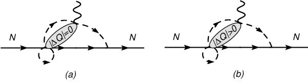
At order most of the new contributing diagrams are formed by attaching a simple pion loop at every vertex in an order diagram, as in fig. (3a-d). In some cases (figs. (3c) and (3d)) this does not create any new zero mode structure, as all of the zero mode information comes from the electromagnetic vertex. However, in fig. (3a) and (3b) the addition of the pion loop to the nucleon-pion vertex creates a new source of zero modes in addition to those from the electromagnetic vertex. The zero mode functions from contributions of this form separate into two groups of diagrams. The first group (characterized by the function as defined in the appendix) contains intermediate nonzero mode pions where charge is conserved separately within both the zero mode and nonzero mode sectors of the theory. The second group (characterized by the function ) contains intermediate zero mode pions which carry electric charge from one vertex to the other. The last two diagrams in fig. (3) are not as simply constructed, but are straightforward to compute. Figure (3e) is the lowest order two loop construction (the electromagnetic vertex can go on either pion loop with an equal contribution) while fig. (3f) is an insertion of the pion kinetic energy operator into an order diagram.

Once the various zero mode functions have been determined, the remaining finite volume nonzero mode Feynman diagrams can be written in the standard way as a four component sum over integers with the zero vector specifically removed. Using the Abel-Plana formula, the fourth component of this vector sum can be written as an infinite volume integral plus finite volume corrections. As shown in ref. [15], due to the nature of the HBChPT propagators, these correction terms will be negligible until at least order and so can be ignored. Using this fact, the diagrams can be determined by integrating over the time component of the momentum and then summing over the remaining spatial components. To perform the sums that arise, one can explicitly expand them in powers of to the order desired, resulting in purely numerical sums (expressed below as coefficients defined in the appendix).
Calculating the contribution from each of the graphs given in figs. (1-3) results in:
| (11) | |||||
| (12) | |||||
| (13) | |||||
| (14) | |||||
| (15) | |||||
with
| (16) |
where the subscript refers to the order in of the contribution. The zero mode functions , , , and as well as the coefficients , , , , , and are defined in the appendix. The pion mass also has a zero mode contribution that has been previously calculated[8] which effects the replacement . The zero mode structure of this replacement is the same as that from the tadpole diagram in fig. (2g) and indeed . Note that the infinite volume portions of the order contributions enter at order , and are the first two terms in .
IV Discussion and Conclusion
We have computed the nucleon magnetic moment in the regime to order . In doing so, two new zero mode functions have been calculated, and . Both of these functions have intriguing features, as each stem from diagrams with two separate vertices that produce zero modes. The zero mode effects contained in the function are generated from zero mode fields that connect the vertices but do not carry charge, as shown in fig. (4a). This is in contrast to the zero modes encapsulated in the function , as they connect and carry charge between the two vertices, as shown in fig. (4b). When writing down contributing diagrams where the zero modes have been removed and placed in the function the diagrams will appear to violate local charge conservation. In fact, charge is locally conserved when the zero modes are included. The form of the function , as shown in fig. (5), is easy to understand. As the zero mode fluctuations become damped and contributions of this type disappear due to charge conservation in the nonzero mode pions, while as the charged zero modes will become increasingly important.
The behavior of the zero mode function is unique because it changes sign as , raising an interesting possibility. For a given choice of spatial volume and pion mass, the temporal dimension of a lattice calculation could be chosen such that was zero, thus removing these contributions from the calculation. In addition, previous studies (see refs. [17, 33, 34]) have discussed the changes that occur in the coefficients and in asymmetric spatial volumes. Specifically, these coefficients can be either enhanced or made to vanish with the correct choice of spatial dimensions. If one was to combine these spatial dimension effects on the coefficients with the temporal dimension effects on the zero mode functions one could design a lattice with a significant degree of control over the contribution of certain graphs.
Due to the increased complexity of lattice calculations involving electromagnetism over lattice calculations with pure QCD, the lattice theorist may be tempted to forgo working on quantities such as the magnetic moment in favor of quantities such as the axial charge. However, the electromagnetic properties of the nucleons are some of the most precisely measured quantities in physics, and as such an important test of lattice QCD will be the reproduction of these values. Because of this, lattice calculations of the nucleon magnetic moment in the -regime will be of importance in the coming years. Furthermore, configurations used to calculate quantities such as the axial charge can also be used to calculate the magnetic moment. In fact, calculating both quantities simultaneously and performing the appropriate correlated statistical analysis on each would be a powerful tool for determining the infinite volume low energy coupling coefficients , , and as well as the magnetic couplings , , , and . With the above results for the magnetic moment and previous results[15] for the axial charge, both quantities can be coherently analyzed in the -regime.
Acknowledgements.
The author would like to thank M. Savage, W. Detmold, and B. Smigielski for many useful discussions.Appendix A Zero Mode Functions
The zero mode functions (with ) calculated for the contributing diagrams are:
| (17) | |||||
| (18) | |||||
| (19) | |||||
| (20) |
Of these functions and have been calculated previously in refs. [15, 8]. The functions and are new to this paper and are generated from contributions of the type shown in figs. (3a) and (3b). These functions are plotted in fig. (5).

Appendix B Sums
For the calculation of the diagrams given above several sums will be important. Many of these sums have been calculated previously [35, 36, 17, 37] and the divergent sums are defined through dimensional regularization:
| (21) |
The sum that needs to be evaluated for the two loop diagram is more complicated, but can be evaluated using the same general techniques:
| (22) |
References
- [1] E. Jenkins and A. V. Manohar (1991a), talk presented at the Workshop on Effective Field Theories of the Standard Model, Dobogoko, Hungary, Aug 1991.
- [2] E. Jenkins and A. V. Manohar, Phys. Lett. B255, 558 (1991b).
- [3] S. R. Coleman and S. L. Glashow, Phys. Rev. Lett. 6, 423 (1961).
- [4] J. Gasser and H. Leutwyler, Ann. Phys. 158, 142 (1984).
- [5] J. Gasser and H. Leutwyler, Nucl. Phys. B250, 465 (1985).
- [6] E. E. Jenkins, M. E. Luke, A. V. Manohar, and M. J. Savage, Phys. Lett. B302, 482 (1993), eprint hep-ph/9212226.
- [7] M. Luscher, Commun. Math. Phys. 104, 177 (1986a).
- [8] J. Gasser and H. Leutwyler, Phys. Lett. B188, 477 (1987).
- [9] F. C. Hansen, Nucl. Phys. B345, 685 (1990a).
- [10] F. C. Hansen and H. Leutwyler, Nucl. Phys. B350, 201 (1991).
- [11] F. C. Hansen (1990b), bUTP-90-42-BERN.
- [12] P. Hasenfratz and H. Leutwyler, Nucl. Phys. B343, 241 (1990).
- [13] A. Hasenfratz et al., Z. Phys. C46, 257 (1990).
- [14] H. Leutwyler and A. Smilga, Phys. Rev. D46, 5607 (1992).
- [15] B. Smigielski and J. Wasem, Phys. Rev. D76, 074503 (2007), eprint arXiv:0706.3731 [hep-lat].
- [16] S. R. Beane, Phys. Rev. D70, 034507 (2004), eprint hep-lat/0403015.
- [17] W. Detmold and M. J. Savage, Phys. Lett. B599, 32 (2004a), eprint hep-lat/0407008.
- [18] B. C. Tiburzi (2007), eprint arXiv:0710.3577 [hep-lat].
- [19] D. G. Caldi and H. Pagels, Phys. Rev. D10, 3739 (1974).
- [20] U.-G. Meissner and S. Steininger, Nucl. Phys. B499, 349 (1997), eprint hep-ph/9701260.
- [21] L. Durand and P. Ha, Phys. Rev. D58, 013010 (1998), eprint hep-ph/9712492.
- [22] T. R. Hemmert and W. Weise, Eur. Phys. J. A15, 487 (2002), eprint hep-lat/0204005.
- [23] D. B. Leinweber, R. M. Woloshyn, and T. Draper, Phys. Rev. D43, 1659 (1991).
- [24] T. Draper, K. F. Liu, D. B. Leinweber, and R. M. Woloshyn, Nucl. Phys. A527, 531c (1991).
- [25] V. Gadiyak, X. D. Ji, and C. Jung, Nucl. Phys. Proc. Suppl. 106, 296 (2002).
- [26] M. Gockeler et al. (QCDSF), Phys. Rev. D71, 034508 (2005), eprint hep-lat/0303019.
- [27] M. Gockeler et al., Eur. Phys. J. A32, 445 (2007a), eprint hep-lat/0609001.
- [28] M. Gockeler et al. (QCDSF) (2007b), eprint arXiv:0709.3370 [hep-lat].
- [29] M. Gockeler et al. (QCDSF/UKQCD), PoS. LATTICE2007 (2007c), eprint arXiv:0710.2159 [hep-lat].
- [30] C. Alexandrou, G. Koutsou, J. W. Negele, and A. Tsapalis, Phys. Rev. D74, 034508 (2006), eprint hep-lat/0605017.
- [31] M. E. Luke and A. V. Manohar, Phys. Lett. B286, 348 (1992), eprint hep-ph/9205228.
- [32] V. Bernard, N. Kaiser, J. Kambor, and U. G. Meissner, Nucl. Phys. B388, 315 (1992).
- [33] W. Detmold and M. J. Savage, Nucl. Phys. A743, 170 (2004b), eprint hep-lat/0403005.
- [34] X. Li and C. Liu, Phys. Lett. B587, 100 (2004), eprint hep-lat/0311035.
- [35] M. Luscher, Commun. Math. Phys. 105, 153 (1986b).
- [36] A. Edery, J. Phys. A39, 685 (2006), eprint math-ph/0510056.
- [37] S. R. Beane, W. Detmold, and M. J. Savage (2007), eprint arXiv:0707.1670 [hep-lat].