On Hydrodynamic Correlations in Low-Dimensional Interacting Systems

Fabio Franchini

Abstract

Low-dimensional systems are an important field of current theoretical and experimental research. Theoretically, the role of dimensionality has been recognized for many years and dramatic predictions have been made that still await experimental confirmation or are currently under study. Recent technological developments provide many possible realizations of effectively one-dimensional systems. These devices promise to give us access to a new range of phenomena. It is therefore very interesting to develop theoretical methods specific for such systems to model their behavior and calculate the correlators of the resulting theory. Incidentally, one such method exists and is known as Bosonization. It can be applied to one-dimensional systems and effectively describes low energy excitations in a universal way. It was developed in the 1970’s when one-dimensional physics was viewed as a toy model for higher dimensional physics. We use the example of a correlator known as the Emptiness Formation Probability to show that Bosonization fails to describe some long range correlators corresponding to large disturbances (the EFP measures the probability for the ground state of the system to develop a region without particles). We trace this failure to the fact that Bosonization is constructed as a linear approximation of the full theory and we set up to develop a collective description with the required non-linearity. The resulting scheme is essentially a Hydrodynamic paradigm for quantum systems. We show how to construct such a hydrodynamic description for a variety of exactly integrable models and illustrate how it can be used to make new predictions. For the special case of the spin-1/2 XY model we take advantage of the structure of the model to express the EFP as a determinant of a very special type of matrix, known as Toeplitz Matrix. We use the theory of Toeplitz determinants to calculate the asymptotic behavior of the EFP in the XY model and discuss its relation with the criticality of the theory. Finally, we analyze the behavior of a charged particle in a two-dimensional medium filled with point-like magnetic vortices.

December 2006 \advisorAlexander G. AbanovPhysics & Astronomy Department, Stony Brook University \chairmanJacobus VerbaarschotPhysics & Astronomy Department, Stony Brook University \fstmemberDominik SchneblePhysics & Astronomy Department, Stony Brook University \outmemberRobert KonikCondensed Matter Theory Group, BNL

This thesis is based on the work I performed during my graduate studies. Chapters 2 and 3 are devoted to the calculation of a correlator known as Emptiness Formation Probability for the anisotropic XY model. This analysis is based on the work published in [†] and [‡]. In this chapter we also consider the effect on the block entanglement of the factorized ground state wavefunction on a line of the phase-diagram of the model [§]. Chapter 6 describes how to develop a two-fluid description for a system of spin-1/2 electrons in one dimension. This is still a work in progress [ $\star$ ] the ultimate goal of which is to address the problem of calculating the corrections to the exact spin-charge separation of the Luttinger Liquid model. Chapter 7 describes a two-dimensional problem I studied with the help and the advice of Prof.Ã.S. Goldhaber [ $\diamond$ ]. We consider the Aharonov-Bohm effect for a scalar electron entering a medium filled with point-like magnetic vortices pinned to the sites of a square lattice and we consider the effect of such a configuration in the electron wavefunction. In Appendix D we explicitly construct the conserved currents of gradient-less hydrodynamic theories. While the existence of two infinite series of conserved quantities is known for these systems, we have not found such an explicit construction in the literature. This work is still unpublished, as the fundamental origin of these conserved quantities remains unclear (we address this issue in Appendix D but our results are so far inconclusive).

Publications

†

A.G. Abanov and F. Franchini; Phys. Lett. A 316 (2003) 342-349.
“Emptiness Formation Probability for the Anisotropic XY Spin Chain in a Magnetic Field”
(also available on arXiv:cond-mat/0307001).
‡

F. Franchini and A.G. Abanov; J. Phys. A 38 (2005) 5069-5096.
“Asymptotics of Toeplitz Determinants and the Emptiness Formation Probability for the XY Spin Chain”
(also available on arXiv:cond-mat/0502015).
§

F. Franchini, A. R. Its, B.-Q. Jin and V. E. Korepin; to appear in “Proceedings of the 26th International Colloquium on Group Theoretical Methods in Physics”.
“Analysis of entropy of XY Spin Chain”
(also available on arXiv:quant-ph/0606240).

F. Franchini, A. R. Its, B.-Q. Jin, V. E. Korepin, quant-ph/0609098.
“Ellipses of Constant Entropy in the XY Spin Chain”.
$\star$

F. Franchini and A.G. Abanov; In progress.
“Coupling of Spin and Charge Degrees of Freedom in a Hydrodynamic Two-Fluid Approach”.
$\diamond$

F. Franchini and A.S. Goldhaber; In preparation.
“Aharonov-Bohm effect with many vortices”.

Chapter 1 Introduction

Dimensionality has an extremely important role in determining the physics of a system. Since the 1960’s, one-dimensional physics stopped being just a theoretical toy, when excitations with unusual quantum numbers were observed in polyacetylene structures [1]. Later on, in the 1980’s, the discovery of novel effects in two-dimensional systems such as the Quantum Hall Effect, high-temperature superconductivity, and others, brought increasing attention to low-dimensional physics.

In recent years, zero-dimensional (“Quantum Dots”) and one-dimensional (“Quantum Wires”) systems have been implemented in laboratories as well, by effectively confining the electrons in fewer dimensions, with the motion in the transverse directions quantized so that at sufficiently low temperatures they are made energetically prohibited.

From a theoretical point of view, one-dimensional models are particularly interesting, because, in some sense, all 1-D theories are strongly interacting, since particles cannot avoid each other in their motion (all collisions are ‘head-on’). Moreover, in one dimension the distinction between a real scattering event and the effect of quantum statistics is somewhat arbitrary, since it is impossible to exchange two particles without having them interacting.

In addition to these remarkable aspects, there is something special about one-dimensional theories. The special symmetry of having just one spatial dimension together with the temporal one renders one-dimensional models particularly appealing and ‘easy’ to address, while preserving, and sometimes generating new, interesting non-trivial situations. For example, a number of theories are known to be exactly solvable in one dimension, quantum field theory methods are especially powerful and direct, and even the study of gravity is so simple in $1+1$ dimensions that many attempts toward quantum gravity are performed in this lower dimensionality.

In the 1970’s, progress in quantum field theory was always parallel to the study of the corresponding 1-D theory, since the latter was often easier to tackle and provided important clues on the general structure of the methods. These efforts resulted in the development of the field theory method that we call “bosonization” and in the concept of the “Luttinger Liquid”.

1.1 Bosonization, linearization of the spectrum, and Luttinger Liquid concept

One of the most successful methods to study one-dimensional systems is known as “bosonization” [15] which effectively describes low energy excitations in 1-D. One of its biggest advantages is its universality, i.e. the fact that the theory has only two free parameters to be determined microscopically, when possible, and then the structure of the model is always the same for every system.

This universality originates in the fact that the model assumes a linear spectrum, hence its applicability only at energy close to the Fermi points, and this assumption results in a quadratic Lagrangian, even including the interactions.

Physically, the bosonization method provides a very powerful description of the concept of “Luttinger Liquid” (LL) [16] that is commonly employed to describe electrons in one dimension. This is the one-dimensional equivalent of the Fermi Liquid concept, but the fact that in one dimension the Fermi surface collapses to just two points has profound consequences on the physics of the system. Bosonization captures this physics accurately and allows for an easy access to the calculation of many correlation functions, often on very general grounds.

The main limitation of the Luttinger Liquid description and of bosonization is the aforementioned assumption of a linear spectrum, which guarantees its universality. This approximation is extremely reasonable when one is interested in low temperature physics, when only low energy excitations, close to the Fermi points, can contribute. But we would like to argue that there exist some important problems in one-dimensional physics where the non-linearity of the spectrum is essential and non-avoidable. In these cases one needs to go beyond the LL model.

For instance, one of the problems we are going to address is the aforementioned prediction of spin-charge separation. It is a standard result of the Luttinger Liquid description that electrons in a one-dimensional system exist in the form of spin and charge density waves whose dynamics is decoupled at low energies. As the LL model relies on the assumption of a linear spectrum, one can consider the effect of non-linearity of the spectrum on this prediction and this would couple spin and charge degrees of freedom. Any curvature in the spectrum would mix spin and charge degrees of freedom and if one looks at sufficiently high energy excitations the effect of this coupling would be measurable. Unfortunately, a perturbative treatment of the curvature of the spectrum in the bosonized theory generates divergences in the calculation of physical quantities and is notoriously difficult to perform.

The bosonization description of a system is a collective description in which density fluctuations are the effective degrees of freedom considered. To overcome the assumption of linearity, we develop a collective description which retains all the characteristics of the spectrum, while still relying on just a few macroscopical fields.

1.2 The hydrodynamic approach, integrable models, and Bethe Ansatz

In fact, the collective description of quantum systems was suggested long ago by Landau [17]. His method is essentially a hydrodynamic description in which the system is described just by its local density $\rho$ and velocity $v$ . These two fields obey a continuity equation and an Euler equation that depends on the original spectrum of the theory and encodes it into the dynamics of the hydrodynamic parameters.

We are going to apply this hydrodynamic approach to one-dimensional systems at zero-temperatures and show how to derive the hydrodynamic description of different one-dimensional systems [19].

We will pay special attention to integrable systems. These theories are exactly solvable and have an infinite series of conserved quantities. Integrable models are very often good approximations for physical systems and an important test field for theoretical methods, since their high degree of symmetry allows for very controlled calculations.

Results for integrable models are usually derived within the framework of the Bethe Ansatz technique [20, 21, 18]. The Bethe Ansatz provides a way to construct the wavefunctions of the system and to derive many thermodynamic quantities. The knowledge of the wavefunction, though, is implicit and this makes it very hard to calculate the correlation functions of the model. Exact expressions for the correlators are available in terms of determinants of operator valued matrices [18], but these expressions are quite convoluted and are often not of practical use for the evaluation of physical quantities.

We are going to show how the hydrodynamic approach derives directly from the Bethe Ansatz formalism. Therefore, physically relevant correlators involving the density and velocity of the fluid can be more easily evaluated within our approach.

The ability of bosonization to calculate correlators for integrable models has been one of the great advantage of this method in conjunction with the Bethe Ansatz solution which provides the parameters of the theory. Clearly, these correlators are correct up to the linear spectrum approximation. The hydrodynamic approach overcomes this limitation at the cost of dealing with a more complicated collective description, since the hydrodynamic equations are intrinsically non-linear.

1.3 The Emptiness Formation Probability

Throughout most of this work we will concentrate on a particular correlation function known as “Emptiness Formation Probability” (EFP). This correlator measures the probability that a region of the system is depleted of particles [18]. It is clear that a bosonization approach is not suitable for the calculation of the EFP, since particles from everywhere in the spectrum are needed to empty a region of space and the curvature of the spectrum cannot be neglected.

The EFP will be a useful example to show the advantage of the hydrodynamic approach over bosonization when contributions far from the Fermi points are involved. But the importance of the EFP goes beyond its role as an example of such correlators.

The Emptiness Formation Probability was introduced in the development of the determinant representation for correlation functions of the integrable models we mentioned before. A good account of this technique can be found in [18], where is it shown how the Bethe Ansatz solution can be manipulated to produce exact expressions for correlators. A careful analysis of these expressions revealed that the simplest correlator one can construct for integrable models is precisely the EFP.

As we mentioned, the practical calculation of correlators for integrable systems is still an open challenge. Therefore, it is conceivable that the study of the simplest correlator will bring insights helpful to carry on the investigation of other correlators. Probably also for this reason, in recent years a considerable effort has been devoted to the study of the EFP in different systems [18] – [30], but a general method for its calculation is still missing.

We propose the hydrodynamic approach as such a general method for the calculation of the EFP, at least to leading order.

1.4 EFP in different systems

In this section we introduce the EFP for several simple integrable models.

Emptiness Formation Probability:

Let us first consider a one-dimensional quantum system of $N$ particles at zero temperature. The wavefunction of the ground state of the system $\Psi_{G}(x_{1},x_{2},\ldots,x_{N})$ gives the probability distribution $|\Psi_{G}|^{2}$ of having all $N$ particles at given positions $x_{j}$ , where $j=1,\ldots,N$ .

The Emptiness Formation Probability $P(R)$ is defined as the probability of having no particles with coordinates $-R<x_{j}<R$ for every $j$ . Formally we write this as

P(R)={1\over\langle\Psi_{G}|\Psi_{G}\rangle}\int_{|x_{j}|>R}{\displaystyle\rm\mathstrut d}x_{1}\ldots{\displaystyle\rm\mathstrut d}x_{N}\;|\Psi_{G}(x_{1},\ldots,x_{N})|^{2},

(1.1)

or following [18]

P(R)=\lim_{\alpha\to+\infty}\left\langle\Psi_{G}\right|{\rm e}^{-\alpha\int_{-R}^{R}\rho(x)\,{\displaystyle\rm\mathstrut d}x}\left|\Psi_{G}\right\rangle,

(1.2)

where $\rho(x)$ is the particle density operator

\rho(x)\equiv\sum_{j=1}^{N}\delta(x-x_{j}).

(1.3)

Spin chains and lattice fermions:

The EFP can also be defined for spin chains. In these systems we are interested in what is known as the “Probability of Formation of Ferromagnetic Strings” (PFFS), where we are looking for strings of length $n$ in the ground state of the spin chain:

P(n)\equiv\langle 0|\prod_{i=1}^{n}{1-\sigma_{i}^{z}\over 2}|0\rangle,

(1.4)

where $\sigma_{i}^{z}$ is the $z$ -component of the Pauli matrices on the $i$ -th lattice site.

The Jordan-Wigner transformation (2.2-2.4) maps a spin- $1/2$ chain to a one-dimensional lattice gas of spinless fermions. Under this mapping the ferromagnetic string corresponds to a string of empty lattice sites and one can write the EFP

P(R)=\left\langle\prod_{j=-R}^{R}\psi_{j}\psi_{j}^{\dagger}\right\rangle,

(1.5)

where $\psi_{j},\psi_{j}^{\dagger}$ are annihilation and creation operators of spinless fermions on the lattice site $j$ .

Therefore, the PFFS in a spin chain corresponds to the EFP of the corresponding Jordan-Wigner fermion theory. In general, we are going to use the language of particles in this work, so we will generically refer to the EFP even for spin systems, since all EFP results are valid for the corresponding one-dimensional spin systems as well.

Random Matrices:

As a remark, we point out that the EFP (1.1) introduced for a general one-dimensional quantum system is a well-known quantity in the context of the spectra of random matrices [36]. Essentially, it is the probability of having no eigenvalues in some range of the spectrum.

Consider, e.g., the joint eigenvalue distribution for the Circular Unitary Ensemble (CUE). The CUE is defined as an ensemble of $N\times N$ unitary matrices with the ensemble measure given by the de Haar measure. Diagonalizing the matrices and integrating out the unitary rotations, one obtains [61]

\int DU\to\int\prod_{j=1}^{N}{\displaystyle\rm\mathstrut d}\theta_{j}\,\prod_{1\leq j<k\leq N}\left|{\rm e}^{{\rm i}\theta_{j}}-{\rm e}^{{\rm i}\theta_{k}}\right|^{\beta},

(1.6)

where $\beta=2$ for the CUE and ${\rm e}^{{\rm i}\theta_{j}}$ , with $j=1,\ldots,N$ , are the eigenvalues of a unitary matrix.

One can then read the joint eigenvalue distribution as

P_{N}(\theta_{1},\ldots,\theta_{N})={\rm const.}\prod_{1\leq j<k\leq N}\left|{\rm e}^{{\rm i}\theta_{j}}-{\rm e}^{{\rm i}\theta_{k}}\right|^{\beta}.

(1.7)

We can now introduce the probability of having no eigenvalues on the arc $-\alpha<\theta<\alpha$ as

P(\alpha)={1\over{\cal N}}\int_{\theta_{j}\notin[-\alpha,\alpha]}\prod_{j=1}^{N}{\displaystyle\rm\mathstrut d}\theta_{j}\,\prod_{1\leq j<k\leq N}\left|{\rm e}^{{\rm i}\theta_{j}}-{\rm e}^{{\rm i}\theta_{k}}\right|^{\beta}.

(1.8)

In the theory of Random Matrices, this quantity is known as $E_{\beta}(0,\alpha)$ , using the notations of [61], and is clearly equivalent to the EFP once one identifies energy eigenvalues and particles. For orthogonal, unitary, and symplectic circular ensembles the joint eigenvalue distribution is given by (1.7) with $\beta=1,2,4$ respectively, where $\beta=2$ corresponds to free fermions, while $\beta=1,4$ are particular cases of the EFP in the Calogero-Sutherland model [61].

1.5 Some implementations of One-Dimensional systems

While one-dimensional physics has been an active sector of research in theoretical studies, only recently laboratories around the world have been able to build and study devices where the motion of electrons is effectively limited to just one dimension and where sufficient control is available to explore different regimes and phases. This allows to finally test in experiments the theoretical prediction on 1-D models. We present an overview of some systems and some experiments where Luttinger liquid behavior has been confirmed and discuss whether curvature effects, like the correction to exact spin-charge separation, can be observed.

GaAs/AlGaAs quantum wires:

One dimensional quantum wires are realized by cleaved edge overgrowth on a GaAs/AlGaAs heterostructures. These wires are in the ballistic regimes and Luttinger Liquid behavior has been confirmed by several experiments, for instance by measuring deviation from exact quantization of the conductance against the theoretical predictions [2]. Recently, efforts have been devoted in observing signatures of spin-charge separation in these quantum wires [3], but the results are so far non-conclusive. The experiment was conducted on two parallel ballistic wires, by measuring the tunneling current: the measurements were in qualitative agreement with the theory, but one of the two predicted charge modes was not observed. It is conceivable that in the future a similar setup could be implemented to test Coulomb drag effects [4], that would carry a clear signs of spectrum curvature, but attempts in this direction require a level of sophistication beyond the technology available today.

Carbon nanotubes:

Single-wall and multi-wall carbon nanotubes are excellent examples of effectively one-dimensional systems [5, 6]. Different realizations of the tubes generated metallic, insulating, semi-metallic and semi-conducting wires. Luttinger liquid behavior of metallic carbon nanotubes have been demonstrated by measuring tunneling amplitudes into the wires through STM experiments [5]. The conductance and differential conductance followed power law behaviors as functions of temperatures and bias voltages, and the exponents were found to be in good agreement with the theory. For semi-metallic wires the description of electrons in terms of Majorana Fermions is almost exact in that the spectrum is linear near the conical point with very good approximation. In the metallic regimes, the Fermi points move away from this point, but we do not expect it to be possible to observe the effect of curvature in these systems with the present technology.

Organic conducting molecules:

Some organic molecules, like polyacetylene, can be used as one-dimensional wires. The main limitation in experiments with organic molecules is the lack of control in the preparation of the system, due to the fact that the molecules have a predefined structure. Therefore, one has to look for the right molecule that could fit a model and there is no a generic set-up that can be used to test different regimes. Polyacetylene, for instance, is a one-dimensional gapped insulator and therefore it cannot be used to test Luttinger liquid behaviors [1]. Conductance studies on Bechgaard salts fibers show the power law behaviors one expects from a Luttinger liquid, but the data are hard to quantitatively match with the theory, due to the complexity of the systems [8]. Evidence for spin-charge separation effects in these salts have been gathered by comparing charge and thermal conductivity, but for a clear interpretation of the results we would need to know these systems better than we currently do.

One-dimensional metallic chains:

For a long time now, one dimensional metallic chains like $Au$ atoms on $Si(111)$ , $Sr_{2}CuO_{3}$ and $SrCuO_{2}s$ have been under investigation, trying to measure evidences of spin-charge separation, but results were not conclusive [9]. Recently, a clear signature of spin-charge separation has been reported using Angle-Resolved PhotoEmission (ARPES) data [10]. They reconstructed the spectral function, which showed two distinct peaks corresponding to the spin and charge contributions in quantitative agreement with the theoretical prediction. There was, however, a significant portion of the spectral function unaccounted by theoretical models, resulting in an unexpected broadening of the peaks. It is possible that this effect is due to the coupling between spin and charge degrees of freedom arising from the spectrum curvature.

Cold atomic gases:

In recent years, impressing technological developments have allowed to cool atomic systems confined in optical traps to unprecedented low temperatures. Since the first observation of Bose-Einstein condensation [11], temperatures have kept dropping, allowing the observation of new physical phenomena. An active field of research focuses on atomic gasses effectively trapped in one-dimensional geometries. It is believed that many solid state physics can be mimicked by these systems and that it would be possible to study them at much lower temperatures than their condensed matter counterparts [12]. Most successful have been experiments with bosons, with the recent realization of a Tonks-Girardeau gas, i.e. a gas of bosons with such strong repulsion that at low enough temperatures and densities exhibit fermionic behavior [13]. It is also expected that a one-dimensional Tonks gas would exhibit Luttinger Liquid behavior and some evidence is already available supporting this prediction [14]. Direct experiments with fermionic gasses need to decrease the temperatures by about two orders of magnitudes compared to the current status in order to realize a Luttinger liquid system, but the improvements in experimental techniques indicate that this goal is probably not far in the future. Indeed, one-dimensional cold atomic gasses are really promising for the investigation of curvature effects of the spectrum in the near future, because these systems allow for a more direct manipulation of the excitations, compared to equivalent solid state systems.

1.6 Outlook of the thesis work

In Chapter 2 we introduce the spin- $1/2$ anisotropic XY model, an important integrable spin chain model in one dimension. In this chapter we analyze the model, study its rich phase diagram and derive the fundamental correlators of the model. The XY model is arguably the simplest integrable model with a non-trivial phase diagram and a perfect candidate for the study of the EFP.

In Chapter 3 we undertake this study and show that for this system the EFP $P(n)$ can be expressed exactly as the determinant of a $n\times n$ matrix. This matrix belong to a class of very special matrices known as Toeplitz Matrices and the asymptotic behavior of their determinant has been studied extensively by mathematicians. We use the results of the theory of Toeplitz determinants to calculate the asymptotic behavior of the EFP in the different regions of the phase-diagram of the model. We find that the EFP decays exponentially in most of the phase diagram and only for the isotropic case studied in [24] is the decay Gaussian. On the critical lines we observe an additional power-law correction to the exponential or Gaussian decay. We employ a bosonization approach to interpret the crossover from the Gaussian to the exponential decay with universal exponents. These results are original and first appeared in [30].

In Chapter 4 we introduce the hydrodynamic approach. We first analyze the hydrodynamic description of free fermions and then proceed to show the technique in its generality and how to obtain the internal energy of integrable systems from the Bethe Ansatz. We also show that the linearization of the hydrodynamic theory produces the traditional bosonization.

In Chapter 5 we show how to derive the leading asymptotic behavior of the EFP for some Galilean invariant systems. This calculation is performed at a semi-classical level, where the EFP is calculated as the probability of a rare fluctuation (“instanton”). We demonstrate that bosonization is insufficient to quantify the EFP. Using the hydrodynamic approach we calculate the EFP to leading order for Free Fermions and for Calogero-Sutherland particles.

In Chapter 6 we analyze the prediction of spin-charge separation in one dimension. First, we show the limitations of the bosonization approach in dealing with the correction to exact spin-charge separation. Then we develop a hydrodynamic description for fermions with contact repulsion. While our ultimate goal is to address the problem of evaluating the corrections to exact spin-charge separation, this is still a work in progress and we can only show how to implicitly construct the hydrodynamic description of this model from its Bethe Ansatz solution.

In Chapter 7 we address a problem very different from the rest of the thesis. It is a single-particle problem in two dimensions. We study the behavior of a scalar particle in a medium filled with point-like magnetic fluxes (vortices) pinned on the sites of a square lattice. By assuming the strength of the fluxes to be all equal to half of the quantum flux unit, we are able to construct a wavefunction of the system, showing that the spectrum of such a system is discrete. Moreover, we are able to show that a zero-energy particle entering such a medium would decay exponentially. This means that an array of vortices could be used to trap a particle and this bound state would have a topological nature. As far as we know, this is the first time that the existence of such a bound state is suggested.

Finally, in Chapter 8 we will discuss the results of this thesis, the problems that remain open and the directions for further research.

We include appendices to supplement the analysis of the main text.

Appendix A is a recapitulation of known results on the EFP calculated for various integrable models.

Appendix B contains a brief review of the results of the theory of Toeplitz determinants, which is extensively used in the evaluation of the asymptotic behavior of the correlation functions of the XY model, including the EFP we study in Chapter 3.

Appendix C is a very brief introduction to the Bethe Ansatz technique where we gather some results we need as an input for the hydrodynamic description of integrable models.

In Appendix D we construct the conserved quantities of gradient-less hydrodynamic theories. The integrability of Galilean invariant hydrodynamic models without gradient correction is a little-known fact discovered in the 1980’s. Here we explicitly construct the integrals of motion for the first time and we attempt to clarify the origin of this integrability.

Chapter 2 The Spin-1/2 Anisotropic XY Model

The One-Dimensional Spin-1/2 Anisotropic XY spin chain is arguably one of the simplest non-trivial quantum integrable models. The reason for this simplicity lies in the fact that it can be reduced to a free fermions model.

The XY model describes a one dimensional lattice system, where each lattice site is occupied by a spin-1/2 quantum degree of freedom interacting with its neighbors. The allowed interaction involves only the X and Y components of the spins. In addition, we consider the presence of an external transverse magnetic field interacting with the Z component of the spins.

Using what is known as a “Jordan-Wigner Transformation” the spin degrees of freedom can be mapped into spin-less fermions, so that the model describes lattice fermions with a quadratic Hamiltonian. The Hamiltonian being quadratic, a “Bogoliubov Rotation” defines “Bogoliubov Quasi-Particles” in terms of which the model reduces to lattice free fermions.

The apparent simplicity of the model does not mean that it is trivial, as these quasi-particles are non-local in terms of the original degrees of freedom. Therefore, every quantity that one wants to calculate for the original model has a non-trivial expression in terms of the free fermions.

A great simplification comes from the fact that for the XY model these non-trivial expressions can often be expressed as determinants of matrices with remarkable symmetries. These matrices are known at “Toeplitz Matrices” and a rich mathematical literature has been devoted to the study of the asymptotic behaviors of their determinant. We will make extensive use of these results on Toeplitz determinants.

The anisotropic XY spin-1/2 chain in a transverse magnetic field is defined by the Hamiltonian

H=\sum_{i=1}^{N}\left[\left({1+\gamma\over 2}\right)\sigma_{i}^{x}\sigma_{i+1}^{x}+\left({1-\gamma\over 2}\right)\sigma_{i}^{y}\sigma_{i+1}^{y}\right]-h\sum_{i=1}^{N}\sigma_{i}^{z},

(2.1)

where $\sigma_{i}^{\alpha}$ , with $\alpha=x,y,z$ , are the Pauli matrices which describe spin operators on the $i$ -th lattice site of the spin chain and, for definiteness, we require periodic boundary conditions: $\sigma_{i}^{\alpha}=\sigma_{i+N}^{\alpha}$ ( $N>>1$ ).

We are interested in this model because of its rich phase-diagram. The model depends on two parameters, the external magnetic field $h$ and the anisotropy parameter $\gamma$ controlling the relative strength of the interaction between the X and Y components of the spins. By varying these parameters the system crosses several quantum phase transitions (QPT). The rich structure of its phase diagram is in contrast with the fair simplicity of the model and makes it an excellent candidate for examination in connection with QPT.

This is one of the reasons for which the XY model is one of the most studied in the growing field of quantum computing and quantum information.

In section 2.1 we introduce the model, and show its different formulations in terms of spins and spinless fermions, and we analyze its phase-diagram. In section 2.2 we derive the fundamental correlators for the model. In this section we will also give an overview of the results of McCoy and co-authors [31] to better understand the structure of this model in preparation for the next chapter where we will calculate the EFP for the XY model [24, 30].

The XY model was first solved by Lieb, Schultz and Mattis in [32] without the external magnetic field. McCoy and co-authors [31] were the first to develop the theory of Toeplitz determinants in connection with the study of the XY spin chain in the external field and to exploit these structures to derive the fundamental correlators of the model.

2.1 The model and its phases

The XY model described in (2.1) has been solved in [32] in the case of zero magnetic field and in [31] in the presence of a magnetic field. We follow the standard prescription [32] and reformulate the Hamiltonian (2.1) in terms of spinless fermions $\psi_{i}$ by means of a Jordan-Wigner transformation:

$\displaystyle\sigma_{j}^{+}$	$\displaystyle=$	$\displaystyle\psi_{j}^{\dagger}\>{\rm e}^{{\rm i}\pi\sum_{k<j}\psi_{k}^{\dagger}\psi_{k}}=\psi_{j}^{\dagger}\>\prod_{k<j}\left(2\psi_{k}^{\dagger}\psi_{k}-1\right),$	(2.2)
$\displaystyle\sigma_{j}^{-}$	$\displaystyle=$	$\displaystyle{\rm e}^{-{\rm i}\pi\sum_{k<j}\psi_{k}^{\dagger}\psi_{k}}\>\psi_{j}=\prod_{k<j}\left(2\psi_{k}\psi_{k}^{\dagger}-1\right)\>\psi_{j},$	(2.3)
$\displaystyle\sigma_{j}^{z}$	$\displaystyle=$	$\displaystyle 2\psi_{j}^{\dagger}\psi_{j}-1,$	(2.4)

where, as usual,

\sigma^{\pm}={\sigma^{x}\pm i\sigma^{y}\over 2}.

(2.5)

The Hamiltonian in terms of these spinless fermions becomes:

H=\sum_{i=1}^{N}\left(\psi_{i}^{\dagger}\psi_{i+1}+\psi_{i+1}^{\dagger}\psi_{i}+\gamma\;\psi_{i}^{\dagger}\psi_{i+1}^{\dagger}+\gamma\;\psi_{i+1}\psi_{i}-2h\;\psi_{i}^{\dagger}\psi_{i}\right)

(2.6)

and in Fourier space it reads ( $\psi_{j}=\sum_{q}\psi_{q}{\rm e}^{{\rm i}qj}$ ):

H=\sum_{q}\left[2\left(\cos\!q-h\right)\psi_{q}^{\dagger}\psi_{q}+{\rm i}\gamma\sin\!q\>\psi_{q}^{\dagger}\psi_{-q}^{\dagger}-{\rm i}\gamma\sin\!q\>\psi_{-q}\psi_{q}\right].

(2.7)

We can now diagonalize this Hamiltonian by means of a Bogoliubov transformation

\chi_{q}=\cos\!{\vartheta_{q}\over 2}\>\psi_{q}+{\rm i}\sin\!{\vartheta_{q}\over 2}\>\psi_{-q}^{\dagger},

(2.8)

which mixes the Fourier components with “rotation angle” $\vartheta_{q}$ defined by

e^{{\rm i}\vartheta_{q}}=\frac{1}{\varepsilon_{q}}(\cos q-h+{\rm i}\gamma\sin q).

(2.9)

In terms of these new Bogoliubov quasi-particles $\chi_{q}$ the Hamiltonian (2.7) has diagonal form

H=\sum_{q}\varepsilon_{q}\chi_{q}^{\dagger}\chi_{q}

(2.10)

with the quasiparticle spectrum

\varepsilon_{q}=\sqrt{\left(\cos q-h\right)^{2}+\gamma^{2}\sin^{2}q}.

(2.11)

Refer to caption — Figure 2.1: Phase diagram of the XY Model (only the part $\gamma\geq 0$ is shown). The theory is critical for $h=\pm 1$ ( $\Omega_{\pm}$ ) and for $\gamma=0$ and $|h|<1$ ( $\Omega_{0}$ ). The line $\Gamma_{I}$ represents the Ising Model in transverse field. On the line $\Gamma_{E}$ the ground state of the theory is a product of single spin states.

A system is said to be “critical” when its spectrum is gapless, i.e. when one can excite particles from the Fermi Sea without spending energy. When a system becomes critical, it undergoes a “Quantum Phase Transition (QPT)”. QPTs are zero-temperature analogs of traditional phase transitions. QPTs are characterized by singularities in thermodynamic quantities and by correlators having a characteristic algebraic behavior. The effective theory is scale invariant and in one dimension can be described through Bosonization. QPTs are a very active field of research, especially since experiments can reach low enough temperatures where their signatures are observable.

We recognize from (2.11) that the theory is critical, i.e. gapless, for $h=\pm 1$ or for $\gamma=0$ and $|h|<1$ .

In Fig. 2.1 we show the phase diagram of the XY model, which has obvious symmetries $\gamma\to-\gamma$ and $h\to-h$ ¹¹ 1 In the next chapter we will analyze the EFP for the XY and we will see that this correlator breaks the latter symmetry.. The phase diagram has both critical and non-critical regimes. Three critical lines $\Omega_{0}$ (Isotropic XY model: $\gamma=0$ , $|h|<1$ ) and $\Omega_{\pm}$ (critical magnetic field: $h=\pm 1$ ) divide the phase diagram into three non-critical domains, $\Sigma_{-}$ , $\Sigma_{0}$ , and $\Sigma_{+}$ ( $h<-1$ , $-1<h<1$ , and $h>1$ respectively). Fig. 2.1 also shows the line $\gamma=1$ ( $\Gamma_{I}$ ) corresponding to the Ising model in transverse magnetic field and the line $\gamma^{2}+h^{2}=1$ ( $\Gamma_{E}$ ) on which the wavefunction of the ground state is factorized into a product of single spin states [34].

2.2 The correlators of the model

In this section we review the derivation of the fundamental correlators for the XY model at zero temperature following McCoy and co-authors [31].

The ground state $|0\rangle$ of the model in terms of the Bogoliubov quasi-particles in (2.10) is defined as

\chi_{q}|0\rangle=0\qquad\forall q

(2.12)

i.e. it is the conventional ground state of free fermions. The correlators for this theory are easily found to be

$\displaystyle\langle 0\|\chi^{\dagger}_{q}\chi_{k}\|0\rangle$	$\displaystyle=$	$\displaystyle\delta_{k,q},$	(2.13)
$\displaystyle\langle 0\|\chi_{q}\chi^{\dagger}_{k}\|0\rangle$	$\displaystyle=$	$\displaystyle 0,$	(2.14)
$\displaystyle\langle 0\|\chi_{q}\chi_{k}\|0\rangle$	$\displaystyle=$	$\displaystyle 0,$	(2.15)
$\displaystyle\langle 0\|\chi^{\dagger}_{q}\chi^{\dagger}_{k}\|0\rangle$	$\displaystyle=$	$\displaystyle 0.$	(2.16)

This vacuum is the ground state for the XY model, but it is not so simple when expressed in terms of physical particles. The Hamiltonian (2.7) contains superconducting-like terms, so its ground state is non-trivial. One can invert the Bogoliubov transformation (2.8)

\psi_{q}=\cos\!{\vartheta_{q}\over 2}\>\chi_{q}-{\rm i}\sin\!{\vartheta_{q}\over 2}\>\chi_{-q}^{\dagger}

(2.17)

to calculate the fundamental correlators in terms of physical fermions:

$\displaystyle\langle 0\|\psi^{\dagger}_{q}\psi_{k}\|0\rangle=\sin^{2}{\vartheta_{q}\over 2}\>\delta_{k,q}$	$\displaystyle=$	$\displaystyle{1-\cos{\vartheta_{q}}\over 2}\>\delta_{k,q},$	(2.18)
$\displaystyle\langle 0\|\psi_{q}\psi^{\dagger}_{k}\|0\rangle=\cos^{2}{\vartheta_{q}\over 2}\>\delta_{k,q}$	$\displaystyle=$	$\displaystyle{1+\cos{\vartheta_{q}}\over 2}\>\delta_{k,q},$	(2.19)
$\displaystyle\langle 0\|\psi_{q}\psi_{k}\|0\rangle=-{\rm i}\>\cos{\vartheta_{q}\over 2}\sin{\vartheta_{q}\over 2}\>\delta_{k,q}$	$\displaystyle=$	$\displaystyle-{\rm i}\>{\sin{\vartheta_{q}}\over 2}\>\delta_{k,q},$	(2.20)
$\displaystyle\langle 0\|\psi^{\dagger}_{q}\psi^{\dagger}_{k}\|0\rangle={\rm i}\>\cos{\vartheta_{q}\over 2}\sin{\vartheta_{q}\over 2}\>\delta_{k,q}$	$\displaystyle=$	$\displaystyle{\rm i}\>{\sin{\vartheta_{q}}\over 2}\>\delta_{k,q}.$	(2.21)

Now, the two-point fermionic correlators are easy to obtain by Fourier transform. In the thermodynamic limit they read [32, 31]

	$\displaystyle F_{jk}$	$\displaystyle\equiv$	$\displaystyle{\rm i}\langle 0\|\psi_{j}\psi_{k}\|0\rangle=-{\rm i}\langle 0\|\psi_{j}^{\dagger}\psi_{k}^{\dagger}\|0\rangle=\int_{0}^{2\pi}{{\displaystyle\rm\mathstrut d}q\over 2\pi}\;\frac{\sin\vartheta_{q}}{2}{\rm e}^{{\rm i}q(j-k)},$		(2.22)
	$\displaystyle G_{jk}$	$\displaystyle\equiv$	$\displaystyle\langle 0\|\psi_{j}\psi_{k}^{\dagger}\|0\rangle=\int_{0}^{2\pi}{{\displaystyle\rm\mathstrut d}q\over 2\pi}\;\frac{1+\cos\vartheta_{q}}{2}{\rm e}^{{\rm i}q(j-k)}.$		(2.23)

These correlators will be fundamental in our calculation of the EFP in the next chapter.

To calculate the correlation functions for the original spin chain model (2.1),

\rho^{\nu}_{lm}\equiv\langle 0\left|\sigma^{\nu}_{l}\>\sigma^{\nu}_{m}\right|0\rangle\qquad\nu=x,y,z,

(2.24)

we need more work. We follow [32] and express these correlators in terms of spin lowering and raising operators (2.5):

$\displaystyle\rho^{x}_{lm}$	$\displaystyle=$	$\displaystyle\langle 0\left\|\left(\sigma^{+}_{l}+\sigma^{-}_{l}\right)\>\left(\sigma^{+}_{m}+\sigma^{-}_{m}\right)\right\|0\rangle,$	(2.25)
$\displaystyle\rho^{y}_{lm}$	$\displaystyle=$	$\displaystyle\langle 0\left\|\left(\sigma^{+}_{l}-\sigma^{-}_{l}\right)\>\left(\sigma^{+}_{m}-\sigma^{-}_{m}\right)\right\|0\rangle,$	(2.26)
$\displaystyle\rho^{z}_{lm}$	$\displaystyle=$	$\displaystyle\langle 0\left\|\left(2\sigma^{+}_{l}\sigma^{-}_{l}-1\right)\>\left(2\sigma^{+}_{m}\sigma^{-}_{m}-1\right)\right\|0\rangle.$	(2.27)

and use (2.2-2.4) to write them using spinless fermions operators.

For instance, let us consider $\rho^{x}_{lm}$ :

$\displaystyle\rho^{x}_{lm}$	$\displaystyle=$	$\displaystyle\langle 0\left\|\left(\sigma^{+}_{l}+\sigma^{-}_{l}\right)\>\left(\sigma^{+}_{m}+\sigma^{-}_{m}\right)\right\|0\rangle$	(2.28)
	$\displaystyle=$	$\displaystyle\langle 0\|\left(\psi^{\dagger}_{l}+\psi_{l}\right)\>\prod_{i=l}^{m-1}\left(2\psi^{\dagger}_{i}\psi_{i}-1\right)\>\left(\psi^{\dagger}_{m}+\psi_{m}\right)\|0\rangle$
	$\displaystyle=$	$\displaystyle\langle 0\|\left(\psi^{\dagger}_{l}-\psi_{l}\right)\>\prod_{i=l+1}^{m-1}\left(2\psi^{\dagger}_{i}\psi_{i}-1\right)\>\left(\psi^{\dagger}_{m}+\psi_{m}\right)\|0\rangle$
	$\displaystyle=$	$\displaystyle\langle 0\|\left(\psi^{\dagger}_{l}-\psi_{l}\right)\>\prod_{i=l+1}^{m-1}\left(\psi^{\dagger}_{i}+\psi_{i}\right)\left(\psi^{\dagger}_{i}-\psi_{i}\right)\>\left(\psi^{\dagger}_{m}+\psi_{m}\right)\|0\rangle,$

where we have used two identities

\sigma_{j}^{+}=\psi_{j}^{\dagger}\>{\rm e}^{{\rm i}\pi\sum_{k<j}\psi_{k}^{\dagger}\psi_{k}}={\rm e}^{-{\rm i}\pi\sum_{k<j}\psi_{k}^{\dagger}\psi_{k}}\>\psi_{j}^{\dagger}

(2.29)

and

{\rm e}^{{\rm i}\pi\psi_{i}^{\dagger}\psi_{i}}=2\psi_{i}^{\dagger}\psi_{i}-1=\left(\psi_{i}^{\dagger}+\psi_{i}\right)\left(\psi_{i}^{\dagger}-\psi_{i}\right)=-\left(\psi_{i}^{\dagger}-\psi_{i}\right)\left(\psi_{i}^{\dagger}+\psi_{i}\right).

(2.30)

Now we define the operators

	$\displaystyle A_{i}$	$\displaystyle\equiv\psi^{\dagger}_{i}+\psi_{i}$			(2.31)
	$\displaystyle B_{i}$	$\displaystyle\equiv\psi^{\dagger}_{i}-\psi_{i}$			(2.32)

which allow us to write the correlators (2.24) as

$\displaystyle\rho^{x}_{lm}$	$\displaystyle=$	$\displaystyle\langle 0\|B_{l}A_{l+1}B_{l+1}\ldots A_{m-1}B_{m-1}A_{m}\|0\rangle$
$\displaystyle\rho^{y}_{lm}$	$\displaystyle=$	$\displaystyle(-1)^{m-1}\langle 0\|A_{l}B_{l+1}A_{l+1}\ldots B_{m-1}A_{m-1}B_{m}\|0\rangle$
$\displaystyle\rho^{z}_{lm}$	$\displaystyle=$	$\displaystyle\langle 0\|A_{l}B_{l}A_{m}B_{m}\|0\rangle.$	(2.33)

We can use Wick’s Theorem to expand these expectation values in terms of two point correlation functions. By noticing that

\langle 0|A_{l}A_{m}|0\rangle=\langle 0|B_{l}B_{m}|0\rangle=0

(2.34)

we write $\rho^{z}_{lm}$ as

	$\displaystyle\rho^{z}_{lm}$	$\displaystyle=$	$\displaystyle\langle 0\|A_{l}B_{l}\|0\rangle\langle 0\|A_{m}B_{m}\|0\rangle-\langle 0\|A_{l}B_{m}\|0\rangle\langle 0\|A_{m}B_{l}\|0\rangle$		(2.35)
		$\displaystyle=$	$\displaystyle H^{2}(0)-H(m-l)H(l-m)$		(2.35)

where

H(m-l)\equiv\langle 0|B_{l}A_{m}|0\rangle={1\over 2}\int_{0}^{2\pi}{{\displaystyle\rm\mathstrut d}q\over 2\pi}\;{\rm e}^{{\rm i}\vartheta_{q}}{\rm e}^{{\rm i}q(m-l)}.

(2.36)

The other two correlators in (2.33) involve more terms. It can be shown [31, 32] that the Wick’s expansion can be expressed as a Pfaffian of a matrix with elements given by expectation values of each combination of two operators.

The Pfaffian of a matrix $M$ is defined as [33]

{\rm Pf}({\bf M})\equiv\sum_{P}(-1)^{P}M_{p_{1}p_{2}}M_{p_{3}p_{4}}\ldots M_{p_{2n-1}p_{2n}},

(2.37)

where $P=\{p_{1},p_{2},\ldots,p_{2n}\}$ is a permutation of $\{1,2,\ldots,2n\}$ , the sum is performed over all possible permutations, and $(-1)^{P}$ is the parity of the permutation.

By using one of the fundamental properties of the Pfaffian:

{\rm Pf}({\bf M})=\sqrt{\det({\bf M})}

(2.38)

we can write the spin correlators (2.33) as $m-l\times m-l$ matrix determinants:

	$\displaystyle\rho^{x}_{lm}$	$\displaystyle=$	$\displaystyle\det\left\|H(i-j)\right\|_{i=l\ldots m-1}^{j=l+1\ldots m},$		(2.39)
	$\displaystyle\rho^{y}_{lm}$	$\displaystyle=$	$\displaystyle\det\left\|H(i-j)\right\|_{i=l+1\ldots m}^{j=l\ldots m-1}$		(2.40)

with matrix elements given by (2.36).

Matrices like (2.39,2.40) are very special. Their entries depend only on the difference between the row and column index, so that the same elements appear on each diagonal. Therefore they look like:

\rho^{x}_{lm}=\rho^{x}(N)=\left|\matrix{H(-1)&H(-2)&H(-3)&\ldots&H(-N)\cr H(0)&H(-1)&H(-2)&\ldots&H(1-N)\cr H(1)&H(0)&H(-1)&\ldots&H(2-N)\cr\vdots&\vdots&\vdots&\ddots&\vdots\cr H(N-2)&H(N-3)&H(N-4)&\ldots&H(-1)\cr}\right|,

(2.41)

\rho^{y}_{lm}=\rho^{y}(N)=\left|\matrix{H(1)&H(0)&H(-1)&\ldots&H(2-N)\cr H(2)&H(1)&H(0)&\ldots&H(3-N)\cr H(3)&H(2)&H(1)&\ldots&H(4-N)\cr\vdots&\vdots&\vdots&\ddots&\vdots\cr H(N)&H(N-1)&H(N-2)&\ldots&H(1)\cr}\right|,

(2.42)

where $N=m-l$ .

Matrices like (2.39,2.40) are known as “Toeplitz Matrices” and a vast mathematical literature has been devoted to the study of the asymptotic behavior of their determinants (“Toeplitz Determinants”). McCoy and co-authors [31] were among the first to develop the theory of Toeplitz determinants in connection to physical systems. They showed that the fundamental correlators for the XY model can be calculated in terms of Toeplitz Determinants. In the next chapter we are going to calculate the Emptiness Formation Probability in the XY model, a non trivial correlator, and we are going to show that it also can be expressed as a Toeplitz determinant.

We will defer an appropriate discussion on the theory of Toeplitz matrices to the next chapter, where we are going to use it to calculate the EFP. Here, we are just going to recap the main results of [31] on the asymptotic behavior of the fundamental spin correlators (2.24).

At zero temperature, the asymptotic evaluation of the Toeplitz determinant in the different regions of the phase diagram for $\rho^{x}(N)$ gives [31]

\rho^{x}(N){\stackrel{{\scriptstyle N\to\infty}}{{\sim}}}\cases{(-1)^{N}{2\over 1+\gamma}\left[\gamma^{2}(1-h^{2})\right]^{1/4}&$|h|<1$, $\gamma>0$\cr(-1)^{N}{2\gamma\over 1+\gamma}{\rm e}^{1/4}2^{1/12}A^{-3}(\gamma N)^{-1/4}&$|h|=1$, $\gamma>0$\cr(-1)^{N}f_{1}(h,\gamma){\lambda^{N}\over\sqrt{N}}&$|h|>1$, $\gamma>0$\cr 0&$\gamma=0$}

(2.43)

where $A=1.282\ldots$ is the Glaisher’s constant, $f_{1}(h,\gamma)$ is some function (see [31]) and

\lambda\equiv{h-\sqrt{h^{2}+\gamma^{2}-1}\over 1-\gamma}.

(2.44)

For $\rho^{y}(N)$ it was found

\rho^{y}(N){\stackrel{{\scriptstyle N\to\infty}}{{\sim}}}\cases{-(-1)^{N}f_{2}(h,\gamma)N^{-3}\lambda^{-2N}&$|h|<\sqrt{1-\gamma^{2}}$, $\gamma>0$\cr 0&$|h|=\sqrt{1-\gamma^{2}}$, $\gamma>0$\cr(-1)^{N}f_{3}(h,\gamma)N^{-1}\left({1-\gamma\over 1+\gamma}\right)^{N}&$\sqrt{1-\gamma^{2}}<|h|<1$, $\gamma>0$\cr-(-1)^{N}{\gamma(1+\gamma)\over 8}{\rm e}^{1/4}2^{1/12}A^{-3}(\gamma N)^{-9/4}&$|h|=1$, $\gamma>0$\cr-(-1)^{N}f_{4}(h,\gamma)N^{-3/2}\lambda^{N}&$|h|>1$, $\gamma>0$\cr 0&$\gamma=0$ .}

(2.45)

Finally, for $\rho^{z}(N)$ we have

\rho^{z}(N){\stackrel{{\scriptstyle N\to\infty}}{{\sim}}}\cases{m_{z}^{2}-f_{5}(h,\gamma)N^{-2}\left({1-\gamma\over 1+\gamma}\right)^{N}&$|h|<\sqrt{1-\gamma^{2}}$, $\gamma>0$\cr m_{z}^{2}&$|h|=\sqrt{1-\gamma^{2}}$, $\gamma>0$\cr m_{z}^{2}-{1\over 2\pi}\lambda^{-2N-2}&$\sqrt{1-\gamma^{2}}<|h|<1$, $\gamma>0$\cr m_{z}^{2}-(\pi N)^{-2}&$|h|=1$, $\gamma>0$\cr 1-{1\over 2\pi}N^{-2}\lambda^{-2N}&$|h|>1$, $\gamma>0$\cr m_{z}^{2}-\left({\sin(N\cos^{-}1h)\over\pi N}\right)^{2}&$|h|<1$, $\gamma=0$\cr{1\over 4}&$|h|>1$, $\gamma=0$}

(2.46)

where $m_{z}^{2}$ is the magnetization:

m_{z}={1\over\pi}\int_{0}^{\pi}{h-\cos q\over\sqrt{(h-\cos q)^{2}+\gamma^{2}\sin^{2}q}}{\displaystyle\rm\mathstrut d}q.

(2.47)

Chapter 3 The EFP for the XY Model

In the previous chapter we introduced the One Dimensional Spin-1/2 Anisotropic XY spin chain in a transverse magnetic field. We studied its phase diagram and we calculated the fundamental correlators of this model. Now we turn our attention to a non-trivial correlator know as Emptiness Formation Probability (EFP) which we are going to study for the XY model.

We introduced the EFP in Chapter 1, where we discussed its significance and importance in the theory of integrable models and in the general problem of calculating correlators in one-dimensional theories.

The XY model is a very interesting model for the study of the EFP for several reasons. As we saw in the previous chapter, the XY spin chain is characterized by a very interesting phase diagram: as we vary its two parameters (the anisotropy and the magnetic field), we move through critical and gapped regions. Previous studies of the EFP focused only on critical phases of various systems and the XY model offers an opportunity to follow the behavior of the EFP across a phase transition.

A second, more technical reason, lies in the relative simplicity of the model. In the previous chapter we showed that the fundamental correlators of the theory can be exactly expressed as determinants of a very special class of matrices known as “Toeplitz Matrices”. We show that the same property holds for the EFP. This is of great advantage, since, despite being considered the simplest correlator for integrable models, the EFP in general does not have a simple expression. Using the theory of “Toeplitz Determinants”, we are able to calculate the asymptotic behavior of the EFP in the various regions of the phase diagram of the XY model.

Most of these results appeared first in [30]. The Toeplitz determinant approach was also used in Ref. [24] for the EFP in the case of the Isotropic XY model (Eq. (2.1) with $\gamma=0$ ). In this latter work it was shown that the EFP decays in a Gaussian way for the critical theory ( $\gamma=0$ , $-1\leq h\leq 1$ ). This case corresponds to one of the two critical lines in the $\gamma-h$ phase diagram of the model (2.1) discussed in the previous chapter. The other line is the critical magnetization line(s) ( $h=\pm 1$ ). In the rest of the two-dimensional $\gamma-h$ phase diagram, the model is non-critical.

For the XXZ spin chain in zero magnetic field, the EFP was found to have a Gaussian decay $P(n)\sim e^{-\alpha n^{2}}$ as $n\to\infty$ in the critical regime at zero temperature and exponential $e^{-\beta n}$ at finite temperature ([28],[29]).

A qualitative argument in favor of Gaussian decay was given in Ref. [23] within a field theory approach. It was argued there that the asymptotics of the EFP are defined by the action of an optimal fluctuation (instanton) corresponding to the EFP. In the critical model, this fluctuation will have a form of an “ $n\times n$ ” droplet in space-time with the area $A\sim n^{2}$ and the corresponding action $S\approx\alpha n^{2}$ which gives the decay $P(n)\sim e^{-\alpha n^{2}}$ . Similarly, at finite temperature the droplet becomes rectangular (one dimension $n$ is replaced by an inverse temperature $T^{-1}$ ) and the action cost is proportional to $n$ , giving $P(n)\sim e^{-\beta n}$ . This argument is based on the criticality of the theory¹¹ 1 More precisely, on the assumption that temporal and spatial dimensions of an instanton scale similarly. and it is interesting to consider whether it could be extended to a non-critical theory. A naïve extension of the argument would give the optimal fluctuation with space-time dimensions $n\times\xi$ where $\xi$ is a typical correlation length (in time) of the theory. This would result in $P(n)\sim e^{-\beta n}$ for non-critical theories, similarly to the case of finite temperature in critical regime. The rate of decay $\beta$ would be proportional to the correlation length of the theory.

In this chapter we examine the relation between the asymptotic behavior of the EFP and criticality using the example of the XY model. Using Toeplitz determinant techniques, we obtain that the EFP is asymptotically exponential in most of the phase diagram according to the naïve expectations and that it is Gaussian only at $\gamma=0$ in agreement with previous works on XXZ spin chains and with Ref. [24]. However, on the critical lines $h=\pm 1$ , in addition to the exponential decay, a pre-exponential power-law factor arises, with a universal exponent. The power-law prefactor is present in the isotropic case as well, but with a different exponent. Using a bosonization approach, we will interpret the transition from Gaussian to exponential decay.

The chapter is organized in the following way: in Section 3 we explain how one can express the EFP as the determinant of a Toeplitz matrix and review our results so that readers who are not interested in derivations can skip the next sections. In Section 3.2 we analyze the exponential decay of the EFP for the non-critical and critical phases of the anisotropic XY Model. In Section 3.3 we derive in detail the asymptotic behaviors, including the pre-exponential factors, of both non-critical and critical parts of the phase diagram. In Section 3.4 we study a special line of the phase diagram on which the ground state is known exactly and compare the explicit results one can obtain using the exact ground state with the asymptotes of the EFP we derived in the previous sections. In Section 3.5 we report on the already known results for the EFP of the isotropic XY model [24]. In Section 3.6 we make contact with Ref. [23] using a bosonization approach to discuss the crossover as a function of $n$ from the Gaussian to the exponential behavior of EFP for the case of small anisotropy $\gamma$ . The following section gives some mathematical details on the calculation of the stationary action in the bosonization approach of Section 3.6 and can be skipped by the reader non interested in the mathematical technique. Section 3.8 presents the analysis of the finite temperature behavior of the EFP, which gives an expected exponential decay. Finally, Section 3.9 will summarize our results. For the reader’s convenience we have collected some results on asymptotic behavior of Toeplitz determinants which are extensively used in the rest of the paper in the Appendix B.

3.1 EFP as a determinant of a Toeplitz Matrix

We introduced the XY model in the previous chapter. In this section we consider the correlator measuring the “Probability of Formation of Ferromagnetic Strings” (PFFS)

P(n)\equiv\langle 0|\prod_{i=1}^{n}{1-\sigma_{i}^{z}\over 2}|0\rangle,

(3.1)

at zero temperature (the non-zero temperature case is deferred to section 3.8). This correlator measures the probability that $n$ consecutive spins will be aligned downwards in the ground state of the system.

In terms of the spinless fermions defined in the previous chapter (2.7), by direct substitution one can express the PFFS (3.1) as the expectation value over the spinless fermions ground state [24]

P(n)=\langle 0|\prod_{j=1}^{n}\psi_{j}\psi_{j}^{\dagger}|0\rangle.

(3.2)

This expression projects the ground state on a configuration without particles on a string of length $n$ and hence gives the meaning to the name “Emptiness Formation Probability”.

Let us now introduce the $2n\times 2n$ skew-symmetric matrix ${\bf M}$ of correlation functions

{\bf M}=\pmatrix{{-{\rm i}\bf F}&{\bf G}\cr-{\bf G}&{\rm i}{\bf F}\cr},

(3.3)

where ${\bf F}$ and ${\bf G}$ are $n\times n$ matrices with matrix elements given by $F_{jk}$ and $G_{jk}$ from (2.22,2.23) respectively. Then, using Wick’s theorem on the r.h.s of (3.2), we obtain the EFP as the Pfaffian of the matrix ${\bf M}$

P(n)={\rm Pf}({\bf M}),

(3.4)

where the Pfaffian was introduced in (2.37). Using one of the properties of the Pfaffian we have

P(n)={\rm Pf}({\bf M})=\sqrt{\det({\bf M})}.

(3.5)

We can perform a unitary transformation

{\bf M^{\prime}}={\bf UMU}^{\dagger}=\pmatrix{0&{\bf S_{n}}\cr-{\bf S_{n}}^{\dagger}&0\cr},\qquad{\bf U}={1\over\sqrt{2}}\pmatrix{{\bf I}&{\bf-I}\cr{\bf I}&{\bf I}\cr},

(3.6)

where ${\bf I}$ is a unit $n\times n$ matrix and ${\bf S_{n}}={\bf G}+{\rm i}{\bf F}$ and ${\bf S_{n}}^{\dagger}={\bf G}-{\rm i}{\bf F}$ . This allows us to calculate the determinant of ${\bf M}$ as

\det({\bf M})=\det({\bf M^{\prime}})=\det({\bf S_{n}})\cdot\det({\bf S_{n}}^{\dagger})=\left|\det({\bf S_{n}})\right|^{2}.

(3.7)

The matrix ${\bf S_{n}}$ is a $n\times n$ Toeplitz matrix (i.e. its matrix elements depend only on the difference of row and column indices [37] like the matrices defined in the previous chapter (2.39,2.40)). The generating function $\sigma(q)$ of a Toeplitz matrix is defined by

({\bf S_{n}})_{jk}=\int_{0}^{2\pi}{dq\over 2\pi}\;\sigma(q){\rm e}^{{\rm i}q(j-k)}

(3.8)

and in our case can be found from (2.22,2.23) as

\sigma(q)={1\over 2}\left(1+{\rm e}^{{\rm i}\vartheta_{q}}\right)={1\over 2}+{\cos q-h+{\rm i}\gamma\sin q\over 2\sqrt{(\cos q-h)^{2}+\gamma^{2}\sin^{2}q}}.

(3.9)

Thus, the problem of the calculation of the EFP

P(n)=\left|\det({\bf S_{n}})\right|,

(3.10)

is reduced (exactly) to the calculation of the determinant of the $n\times n$ Toeplitz matrix ${\bf S_{n}}$ defined by the generating function (3.8,3.9). The representation (3.10) is exact and valid for any $n$ . In our study we are interested in finding the asymptotic behavior of (3.10) at large $n\to\infty$ . ²² 2 The reader might notice that our generating function (3.9) is almost the same as the one analyzed by Barouch et al. in [31] ( $\sigma_{[13]}(q)={\cos q-h+{\rm i}\gamma\sin q\over\sqrt{(\cos q-h)^{2}+\gamma^{2}\sin^{2}q}}$ ). The only difference is the shift by the unity in our expression. This difference changes dramatically the analytical structure of the generating function, in particular, its winding number around the origin, and requires a new analysis of the generated Toeplitz determinants.

Most of these results are derived using known theorems on the asymptotic behavior of Toeplitz determinants. We have collected these theorems in Appendix B. In the following sections we apply them to extract the corresponding asymptotes of $P(n)$ at $n\to\infty$ in the different regions of the phase diagram. Two major distinctions have to be made in this process. For the critical isotropic ( $\gamma=0$ ) XY model, one applies what is known as Widom’s Theorem and finds a Gaussian behavior with a power law prefactor [24]. In the rest of the phase diagram, we apply different formulations of what is known in general as the Fisher-Hartwig conjecture, which always leads to an exponential asymptotic behavior. As expected, we find a pure exponential decay for the EFP in the non-critical regions.

For $h>1$ , the exponential decay is modulated by an additional oscillatory behavior.

At the critical magnetizations $h=\pm 1$ , we discover an exponential decay with a power law pre-factor. Moreover, by extending the existing theorems on Toeplitz determinants beyond their range of applicability, for $h=\pm 1$ we obtain the first order corrections to the asymptotics as a faster decaying power law with the same exponential factor. For $h=1$ , the first order correction is also oscillating, which indicates that the EFP has an oscillatory behavior for $h\geq 1$ .

The reader who is not interested in the mathematical details of our derivations can find the results in Figure 3.1 and in Table 3.1 and skip the following sections to go directly to Sec. 3.6, where we analyze the crossover between the Gaussian behavior at $\gamma=0$ and the asymptotic exponential decay at finite $\gamma$ using a bosonization approach.

3.2 Singularities of $\sigma(q)$ and exponential behavior of the EFP

To derive the asymptotic behavior of the EFP we rely on the theorems on determinants of Toeplitz matrices. These theorems depend greatly on the analytical structure of the generating function (3.9), especially on its zeros and singularities.

Setting $\gamma=0$ in (3.9), we see that for the Isotropic XY model the generating function has only a limited support within its period $[0,2\pi]$ . This case is covered by what is known as Widom’s Theorem and will be considered in Section 3.5.

In the remaining parts of the phase-diagram the generating function has only pointwise singularities (zeros) as it is shown in Fig. 3.2. These cases are treated under a general (not yet completely proven) conjecture known as the Fisher-Hartwig conjecture (FH), which prescribes the leading asymptotic behavior of the Toeplitz determinant to be exponential in $n$ :

P(n){\stackrel{{\scriptstyle n\rightarrow\infty}}{{\sim}}}{\rm e}^{-\beta n}.

(3.11)

While the pre-exponential factors depend upon the particulars of the singularities of the generating function, the exponential decay rate is given in the whole phase diagram ( $\gamma\neq 0$ ) according to FH as

	$\displaystyle\beta(h,\gamma)$	$\displaystyle=$	$\displaystyle-\int_{0}^{2\pi}{{\displaystyle\rm\mathstrut d}q\over 2\pi}\;\log\left\|\sigma(q)\right\|$		(3.12)
		$\displaystyle=$	$\displaystyle-\int_{0}^{\pi}{{\displaystyle\rm\mathstrut d}q\over 2\pi}\;\log\left[{1\over 2}\left(1+{\cos q-h\over\sqrt{\left(\cos q-h\right)^{2}+\gamma^{2}\sin^{2}q}}\right)\right].$		(3.12)

The integral in (3.12) is convergent for all $h$ and all $\gamma\neq 0$ and $\beta(h,\gamma)$ is a continuous function of its parameters.

In Fig. 3.3, $\beta(h,\gamma)$ is plotted as a function of $h$ at several values of $\gamma$ . One can see that $\beta(h,\gamma)$ is continuous but has weak (logarithmic) singularities at $h=\pm 1$ . This is one of the effects of the criticality of the model on the asymptotic behavior of EFP.

These weak singularities are also a manifestation of the rich analytical structure underlying $\beta(h,\gamma)$ and the generating function (3.9). To understand these structures, we interpret the periodic generating function (3.9) as the restriction to the unit circle ( $z={\rm e}^{{\rm i}\theta}$ ) of the complex function

\sigma(z)\equiv{1\over 2}\left(1+{p_{1}(z)\over\sqrt{p_{1}(z)\cdot p_{2}(z)}}\right),

(3.13)

where

	$\displaystyle p_{1}(z)={1+\gamma\over 2z}(z-z_{1})(z-z_{2}),$		(3.14)
	$\displaystyle p_{2}(z)={1+\gamma\over 2z}(z_{1}z-1)(z_{2}z-1)$		(3.15)

with

	$\displaystyle z_{1}={h-\sqrt{h^{2}+\gamma^{2}-1}\over 1+\gamma},$		(3.16)
	$\displaystyle z_{2}={h+\sqrt{h^{2}+\gamma^{2}-1}\over 1+\gamma}.$		(3.17)

The integral in (3.12) can be regarded as a contour integral over the unit circle of the function (3.13). We can deform the contour of integration taking into account the complex structure of the integrand in the various regions (see Fig. 3.4) and express (3.12) as a simpler integral on the real axis (after partial integration and some algebra).

3.2.1 The non-critical regions ( $\Sigma_{\pm}$ and $\Sigma_{0}$ )

3.2.1.1 $\Sigma_{-}$ ( $h<-1$ )

For $h<-1$ , the analytical structure of the integrand of (3.12) is shown in Fig. 3.4a. We re-write the decay rate (3.12) in this region as

\beta(h,\gamma)={1\over 2}\ln\left[{\sqrt{h^{2}+\gamma^{2}-1}-h\over\gamma+1}\right]-\Lambda(h,\gamma)-\Delta(h,\gamma),

(3.18)

where

	$\displaystyle\Lambda(h,\gamma)$	$\displaystyle\equiv$	$\displaystyle\ln\left\|{1\over 2}\left(1-{h\over\|h\|}\sqrt{{1-\gamma\over 1+\gamma}}\right)\right\|,$		(3.19)
	$\displaystyle\Delta(h,\gamma)$	$\displaystyle\equiv$	$\displaystyle\int^{1}_{\|K\|}{{\displaystyle\rm\mathstrut d}x\over 2\pi}{1\over\sqrt{(1-x^{2})(x^{2}-K^{2})}}\left(x+{K\over x}\right)\ln\left\|{x-a\over x+a}\right\|,$		(3.20)

with

	$\displaystyle K$	$\displaystyle\equiv$	$\displaystyle{\sqrt{h^{2}+\gamma^{2}-1}-\gamma\over\sqrt{h^{2}+\gamma^{2}-1}+\gamma},$		(3.21)
	$\displaystyle a$	$\displaystyle\equiv$	$\displaystyle{\sqrt{h^{2}+\gamma^{2}-1}-\gamma\over h-1}.$		(3.22)

This decomposition of $\beta(h,\gamma)$ is especially useful in analyzing the transitions between non-critical and critical regimes. In fact, we will see that the functions $\Lambda(h,\gamma)$ and $\Delta(h,\gamma)$ defined above are universal across the phase diagram (hence the need for the seemingly redundant absolute values in our definitions). The absolute value in the logarithm of the integrand is relevant for $\gamma>1$ , since its argument changes sign and vanishes within the interval of integration ( $a>K$ for $\gamma>1$ ).

3.2.1.2 $\Sigma_{0}$ ( $|h|<1$ )

As before, we can express the contour integral defining $\beta(h,\gamma)$ as a standard integral on the real axis. For $|h|<1$ and $h^{2}+\gamma^{2}>1$ , the structure of the integrand is depicted in Fig. 3.4c and the decay rate is simply

\beta(h,\gamma)=-\Lambda(h,\gamma)-\Delta(h,\gamma),

(3.23)

where $\Lambda(h,\gamma)$ and $\Delta(h,\gamma)$ have already been defined in (3.19,3.20).

For $h^{2}+\gamma^{2}<1$ , the structure is quite different (see Fig. 3.4d). In this region the expression for $\beta(h,\gamma)$ in terms of a real axis integral is complicated. We can write the result as:

$\displaystyle\beta(h,\gamma)$	$\displaystyle=$	$\displaystyle-\Lambda(h,\gamma)-\sqrt{2(1+\gamma)(1-h^{2}-\gamma^{2})}\times$
		$\displaystyle\times\int_{0}^{1}{{\displaystyle\rm\mathstrut d}x\over 2\pi}\left\{4x\arctan\left[{x\over h}\sqrt{1-h^{2}-\gamma^{2}}\right]\left({A(x)+B(x)+C(x)\over\sqrt{1-x^{2}}\sqrt{\sqrt{q(x)}+p(x)}}\right)\right.$
		$\displaystyle\left.\qquad+{h\over\|h\|}2x\ln\left[{h^{2}+(1-h^{2}-\gamma^{2})x^{2}\over(1+\gamma)^{2}}\right]\left({A(x)-B(x)-C(x)\over\sqrt{1-x^{2}}\sqrt{\sqrt{q(x)}-p(x)}}\right)\right\}$

where $\Lambda(h,\gamma)$ was defined in (3.19) and

$\displaystyle A(x)$	$\displaystyle\equiv$	$\displaystyle(1+\gamma){r(x)\over t(x)},$	(3.25)
$\displaystyle B(x)$	$\displaystyle\equiv$	$\displaystyle 2(1+\gamma){s(x)\over t(x)\sqrt{q(x)}},$	(3.26)
$\displaystyle C(x)$	$\displaystyle\equiv$	$\displaystyle(\gamma^{2}-1+2\gamma h^{2}){1\over\sqrt{q(x)}},$	(3.27)

with

$\displaystyle p(x)$	$\displaystyle\equiv$	$\displaystyle(\gamma+1)^{3}-(3\gamma+1)h^{2}+(\gamma-1)(1-h^{2}-\gamma^{2})x^{2},$	(3.28)
$\displaystyle q(x)$	$\displaystyle\equiv$	$\displaystyle(\gamma+1)^{6}-2(3\gamma^{4}+10\gamma^{3}+12\gamma^{2}+6\gamma+1)h^{2}+(9\gamma^{2}+6\gamma+1)h^{4}$	(3.29)
		$\displaystyle+2[\gamma^{4}+2\gamma^{3}-2\gamma-1+(5\gamma^{2}+2\gamma+1)h^{2}](1-h^{2}-\gamma^{2})x^{2}$
		$\displaystyle+(\gamma-1)^{2}(1-h^{2}-\gamma^{2})^{2}x^{4},$
$\displaystyle r(x)$	$\displaystyle\equiv$	$\displaystyle(\gamma+1)^{2}-(2\gamma+1)h^{2}+(1-h^{2}-\gamma^{2})x^{2},$	(3.30)
$\displaystyle s(x)$	$\displaystyle\equiv$	$\displaystyle(\gamma+1)^{4}-(3\gamma^{4}+8\gamma^{3}+9\gamma^{2}+6\gamma+2)h^{2}+(5\gamma^{2}+2\gamma+1)h^{4}$	(3.31)
		$\displaystyle+[(\gamma+1)^{2}-(3\gamma^{2}+6\gamma-1)h^{2}](1-h^{2}-\gamma^{2})x^{2},$	(3.31)
$\displaystyle t(x)$	$\displaystyle\equiv$	$\displaystyle[(\gamma+1+h)^{2}+(1-h^{2}-\gamma^{2})x^{2}][(\gamma+1-h)^{2}+(1-h^{2}-\gamma^{2})x^{2}].$

3.2.1.3 $\Sigma_{+}$ ( $h>1$ )

A calculation similar to the previous ones (see Fig. 3.4f) gives the expression for the decay factor for $h>1$ :

\beta(h,\gamma)={1\over 2}\ln\left[{\sqrt{h^{2}+\gamma^{2}-1}+h\over\gamma+1}\right]-\Lambda(h,\gamma)-\Delta(h,\gamma),

(3.33)

where $\Lambda(h,\gamma)$ and $\Delta(h,\gamma)$ were introduced in (3.19) and (3.20).

One important difference exists in this region: as will be discussed in length later in Section 3.3.1.3, in $\Sigma_{+}$ there are two equivalent representations of the generating function. This ambiguity reflects on the value of $\beta$ , in that the choice of the representation for the generating function determines the branch cuts in Fig. 3.4. We will see that we have to use both values of $\beta$ , which differ only by an imaginary constant:

\beta^{\prime}=\beta+{\rm i}\pi

(3.34)

and this will add an oscillatory behavior to the EFP.

3.2.2 The critical lines ( $\Omega_{\pm}$ )

We can calculate the decay factor $\beta$ at $h=1$ ( $\Omega_{+}$ ) from a limiting procedure on (3.23) or (3.33). At $h=1$ , only $\Delta(h,\gamma)$ is nonvanishing, thus guaranteeing the continuity of $\beta$ across the critical line. From an appropriate limit of (3.20), we calculate the decay rate for $h=1$ as

\beta(1,\gamma)=-\int_{0}^{1}{{\displaystyle\rm\mathstrut d}x\over 2\pi}{1\over\sqrt{1-x^{2}}}\ln\left|{1-\gamma x\over 1+\gamma x}\right|-\ln\left|{1\over 2}\left(1-\sqrt{1-\gamma\over 1+\gamma}\right)\right|.

(3.35)

For $\gamma<1$ , we can expand the logarithm in series and perform the integral:

\beta(1,\gamma<1)={1\over\sqrt{\pi}}\sum_{n=0}^{\infty}{n!\over\Gamma(n+1/2)}{\gamma^{2n+1}\over(2n+1)^{2}}-\ln\left[{1\over 2}\left(1-\sqrt{1-\gamma\over 1+\gamma}\right)\right].

(3.36)

As discussed before in reference to (3.33), the definition of $\beta(1,\gamma)$ is not unique and, as in (3.34), will generate again an oscillatory behavior for the EFP (see later in Sec. 3.3.2.1).

The value of $\beta$ at $h=-1$ can also be obtained from a limiting procedure on (3.20)

\beta(-1,\gamma)=\int_{0}^{1}{{\displaystyle\rm\mathstrut d}x\over 2\pi}{1\over\sqrt{1-x^{2}}}\ln\left|{1-\gamma x\over 1+\gamma x}\right|-\ln\left|{1\over 2}\left(1+\sqrt{1-\gamma\over 1+\gamma}\right)\right|.

(3.37)

Again, for $\gamma<1$ , we can expand the logarithm in series to calculate the integral:

\beta(-1,\gamma<1)=-{1\over\sqrt{\pi}}\sum_{n=0}^{\infty}{n!\over\Gamma(n+1/2)}{\gamma^{2n+1}\over(2n+1)^{2}}-\ln\left[{1\over 2}\left(1+\sqrt{1-\gamma\over 1+\gamma}\right)\right].

(3.38)

As can be seen in Fig. 3.3, the decay factor $\beta$ is continuous across the critical lines, but has a discontinuity of its derivative. As $\beta$ approaches the critical lines, it actually shows a non-analytical behavior leading to a logarithmic singularity:

\beta(h=\pm 1+\epsilon,\gamma)=\beta(\pm 1,\gamma)+{\gamma\over\pi}\;\epsilon\ln|\epsilon|.

(3.39)

The derivative $d\beta/dh$ diverges logarithmically as $h\to\pm 1$ .

Moreover, one can easily notice from the difference between expression (3.23) and (3.33) that even the finite part of the derivative of $\beta(h,\gamma)$ by $h$ is different if one approaches the critical line $h=1$ from above or below, due to the appearance of the additional term in (3.33). The same holds across the critical line $h=-1$ , due to the presence of the first term in (3.18), which doesn’t appear in (3.23).

3.3 The pre-exponential factors

For $\gamma\neq 0$ , the leading behavior of the EFP is always exponential. However, the singularities of the generating function are different in different regions of the phase diagram and we must therefore use different forms of the Fisher-Hartwig conjecture in order to derive the pre-exponential factors and determine the asymptotic behavior of $P(n)$ . We will now show how to obtain the results for each of the regions.

3.3.1 The non-critical regions ( $\Sigma_{\pm}$ and $\Sigma_{0}$ )

3.3.1.1 $\Sigma_{-}$ ( $h<-1$ )

In this region ( $\gamma\neq 0$ , $h<-1$ ) the generating function (3.9) is nonzero for all $q$ (see Fig. 3.2a): this is the simplest case and can be treated using the (rigorously proven) Strong Szegö Limit Theorem, see (B.5). It gives

P(n)=\left|\det({\bf S_{n}})\right|{\stackrel{{\scriptstyle n\rightarrow\infty}}{{\sim}}}{\it E_{-}}(h,\gamma){\rm e}^{-\beta(h,\gamma)n}

(3.40)

with $\beta(h,\gamma)$ given by (3.12) or (3.18) and

{\it E_{-}}(h,\gamma)=\exp\left(\sum_{k=1}^{\infty}k\hat{\sigma}_{k}\hat{\sigma}_{-k}\right),

(3.41)

where $\hat{\sigma}_{k}$ is defined in (B.7) as the $k$ -th Fourier component of the logarithm of $\sigma$ :

	$\displaystyle\hat{\sigma}_{k}$	$\displaystyle\equiv$	$\displaystyle\int_{0}^{2\pi}{{\displaystyle\rm\mathstrut d}q\over 2\pi}\;\left[\log\sigma(q)\right]{\rm e}^{-{\rm i}kq}$		(3.42)
		$\displaystyle=$	$\displaystyle\int_{0}^{2\pi}{{\displaystyle\rm\mathstrut d}q\over 2\pi}\;{\rm e}^{-{\rm i}kq}\log\left(1+{\cos q-h+{\rm i}\gamma\sin q\over\sqrt{\left(\cos q-h\right)^{2}+\gamma^{2}\sin^{2}q}}\right).$		(3.42)

The sum in (3.41) is convergent only for $\gamma\neq 0$ and for $h<-1$ . For $h\geq-1$ , the generating function (3.9) develops singularities which produce $1/k$ contributions to (3.42) that make the sum in (3.41) divergent. Therefore, in the rest of the phase diagram these singularities have to be treated to absorb the harmonic series contributions. Consequently, each region of the phase diagram will involve a different definition for the pre-exponential factor and the ”regularization” procedure will sometimes generate an additional power-law contribution. The result is given by the Fisher-Hartwig conjecture that we must use in the remainder of the phase diagram.

3.3.1.2 $\Sigma_{0}$ ( $|h|<1$ )

As can be noticed from Fig. 3.2c, in $\Sigma_{0}$ ( $\gamma\neq 0$ , $-1<h<1$ ) the generating function $\sigma(q)$ vanishes and its phase has a discontinuity of $\pi$ at $q=\pi$ . The asymptotic behavior of Toeplitz determinants with this type of singularities in the generating function is given by FH, which is actually proven for cases in which only one singularity is present.

We decompose the generating function as in (B.8)

\sigma(q)=\tau(q){\rm e}^{{{\rm i}\over 2}[(q-\pi){\rm\>mod\>}2\pi-\pi]}\left(2-2\cos(q-\pi)\right)^{1/2}

(3.43)

and using (B.9) we obtain

P(n)=\left|\det({\bf S_{n}})\right|{\stackrel{{\scriptstyle n\rightarrow\infty}}{{\sim}}}{\it E_{0}}(h,\gamma)\>{\rm e}^{-\beta(h,\gamma)n}.

(3.44)

The behavior is exponential as before with the decay rate $\beta(h,\gamma)$ from (3.12,3.23), but the pre-exponential factor is different. According to (B.10) it is given by

{\it E_{0}}(h,\gamma)\equiv{E[\tau]\over\tau_{-}(\pi)},

(3.45)

where, as in (B.6) and (B.7)

\displaystyle E[\tau]

\displaystyle=

\displaystyle\exp\left(\sum_{k=1}^{\infty}k\hat{\tau}_{k}\hat{\tau}_{-k}\right)

(3.46)

and

\hat{\tau}_{k}=\hat{\sigma}_{k}-{(-1)^{k}\over k}\;\theta(k).

(3.47)

Here $\theta(k)$ is the usual Heaviside step function. As we mentioned in the previous section, $\hat{\sigma}_{k}$ (3.42) has $1/k$ contributions from singularities of $\sigma(q)$ and the effect of the parametrization (3.43) is to cure (remove) these harmonic series divergences of the prefactor of the EFP in this regime.

3.3.1.3 $\Sigma_{+}$ ( $h>1$ )

In $\Sigma_{+}$ ( $\gamma\neq 0$ , $h>1$ ), $\sigma(q)$ vanishes at $q=0$ and $q=\pi$ and its phase presents two $\pi$ jumps at those points (Fig. 3.2e).

In this case the application of FH leads to some ambiguity, because there exist two representations of the kind (B.8) and one obtains two values for $\beta(h,\gamma)$ using the two representations of the generating function: $\beta_{1}=\beta$ and $\beta_{2}=\beta+{\rm i}\pi$ , with $\beta$ from (3.12) or (3.33). This ambiguity is resolved by the (yet unproven) generalized Fisher-Hartwig conjecture (gFH), which gives EFP as a sum of two terms so that both values of $\beta$ ’s are used (see in the Appendix B.3 or [37]).

The two leading inequivalent parametrizations (B.15) are:

$\displaystyle\sigma(q)$	$\displaystyle=$	$\displaystyle\tau^{1}(q){\rm e}^{{{\rm i}\over 2}[(q-\pi){\rm\>mod\>}2\pi-\pi]}\left(2-2\cos(q-\pi)\right)^{1/2}$	(3.49)
		$\displaystyle\qquad\times{\rm e}^{-{{\rm i}\over 2}[q{\rm\>mod\>}2\pi-\pi]}\left(2-2\cos q\right)^{1/2}$
	$\displaystyle=$	$\displaystyle\tau^{2}(q){\rm e}^{-{{\rm i}\over 2}[(q-\pi){\rm\>mod\>}2\pi-\pi]}\left(2-2\cos(q-\pi)\right)^{1/2}$
		$\displaystyle\qquad\times{\rm e}^{{{\rm i}\over 2}[q{\rm\>mod\>}2\pi-\pi]}\left(2-2\cos q\right)^{1/2}.$

Application of (B.16) gives the asymptotic behavior of the determinants as

\left|\det({\bf S_{n}})\right|{\stackrel{{\scriptstyle n\rightarrow\infty}}{{\sim}}}\left[{\it E^{1}_{+}}(h,\gamma)+(-1)^{n}{\it E^{2}_{+}}(h,\gamma)\right]\>{\rm e}^{-\beta(h,\gamma)n}

(3.50)

with

	$\displaystyle{\it E^{1}_{+}}(h,\gamma)\equiv{E[\tau]\over\tau_{+}(0)\tau_{-}(\pi)},$		(3.51)
	$\displaystyle{\it E^{2}_{+}}(h,\gamma)\equiv{E[\tau]\over\tau_{+}(\pi)\tau_{-}(0)}$		(3.52)

and $\beta(h,\gamma)$ , $E[\tau]$ defined in (3.12,3.46) with

\hat{\tau}_{k}=\hat{\sigma}_{k}-{(-1)^{k}\over k}\;\theta(k)-{1\over k}\;\theta(-k).

(3.53)

Once again, as in the previous section, the effect of the parametrization is to remove the $1/k$ contributions to $\hat{\sigma}_{k}$ (3.42) due to the singularities of the generating function.

We conclude that the non-critical theory presents an exponential asymptotic behavior of the EFP. In the region $\Sigma_{+}$ , however, the EFP in addition has even-odd oscillations

P(n){\stackrel{{\scriptstyle n\rightarrow\infty}}{{\sim}}}{\it E^{1}_{+}}(h,\gamma)\left[1+A_{+}(h,\gamma)\cos(\pi n)\right]\>{\rm e}^{-\beta(h,\gamma)n},

(3.54)

where the exponential decay factor is given by (3.33).

The amplitude of the oscillations is

$\displaystyle A_{+}(h,\gamma)$	$\displaystyle\equiv$	$\displaystyle{\tau_{+}(0)\tau_{-}(\pi)\over\tau_{-}(0)\tau_{+}(\pi)}$	(3.55)
	$\displaystyle=$	$\displaystyle{\tau(0)\over\tau(\pi)}\left({\tau_{-}(\pi)\over\tau_{-}(0)}\right)^{2}$
	$\displaystyle=$	$\displaystyle{h+1\over h-1}\exp\left(4\lim_{\epsilon\rightarrow 0}\oint{{\displaystyle\rm\mathstrut d}z\over 2\pi}{\log\tau(z)\over z^{2}-(1+\epsilon)^{2}}\right),$

where we used (B.11), the definition of $\tau$ and (B.13). We can deform the contour of integration as in Fig. 3.4f and calculate the integral in (3.55) to obtain

A_{+}(h,\gamma)=\sqrt{K(h,\gamma)}={\sqrt{h^{2}-1}\over\sqrt{h^{2}+\gamma^{2}-1}+\gamma}\;,

(3.56)

where $K(h,\gamma)$ was defined in (3.21).

Expression (3.54) for the EFP fits the numerical data remarkably well (see Fig. 3.5) and this fact strongly supports the generalized Fisher-Hartwig conjecture.

One can understand these oscillations as a result of “superconducting” correlations of real fermions described by the Hamiltonian (2.6). Fermions are created and destroyed in pairs of nearest neighbors. At large magnetic fields, the oscillations are due to the fact that the probability of having a depletion string of length $2k-1$ or $2k$ is very similar. Since the magnetic field in (2.6) is essentially a chemical potential for the fermions, the energy cost to destroy a pair of particles is $4h$ : at very big magnetic fields, the amplitude for a pair destruction event is suppressed by a factor of $\gamma\over 4h$ , i.e. a probability of $\gamma^{2}\over 16h^{2}$ . This means that the probability of depletion behaves like:

	$\displaystyle P(2k-1)$	$\displaystyle\sim$	$\displaystyle 2\left({4h\over\gamma}\right)^{-2k}\qquad{\rm and}$
	$\displaystyle P(2k)$	$\displaystyle\sim$	$\displaystyle\left({4h\over\gamma}\right)^{-2k}\;,$		(3.57)

where the factor of two in the first expression is a simple combinatorial factor. The two probabilities in (3.57) can be combined in a single expression:

P(n)=E\left[1+A\cos(\pi n)\right]\left({4h\over\gamma}\right)^{-n},

(3.58)

which is precisely (3.54), with

A=1-{\gamma\over h}+{\rm O}\left({1\over h^{2}}\right).

(3.59)

We can check the correctness of this interpretation by taking the limit of (3.54) for $h>>1,\gamma$ . From (3.12) and (3.56) it is easy to find

	$\displaystyle\beta(h\to\infty,\gamma)$	$\displaystyle=$	$\displaystyle\log{4h\over\gamma}+\;{\rm O}\left({1\over h^{2}}\right)$		(3.60)
	$\displaystyle A_{+}(h\to\infty,\gamma)$	$\displaystyle=$	$\displaystyle 1-{\gamma\over h}+{\rm O}\left({1\over h^{2}}\right)$		(3.61)

in agreement with (3.58,3.59).

Figure 3.5: Results of the numerical calculation of the Toeplitz determinant are shown as points,

P(n)e^{\beta n}

vs.

n

\gamma=1

h=1.1

. The value of

\beta

is obtained numerically from (3.35). The solid line is the analytic result

E(1+(-1)^{n}A)

with

A=0.2182...

from (3.56) and

E=0.6659...

obtained by fitting at large

n

. To make the plot more readable we show only every 11th point (for

n=1,12,23,\ldots

) of the numerical calculation of the determinant. Note that the size of the points is not related to the estimated error in the numerics, which is actually smaller.

3.3.2 The critical lines ( $\Omega_{\pm}$ )

3.3.2.1 $\Omega_{+}$ ( $h=1$ )

For $h=1$ the generating function $\sigma(q)$ vanishes at $q=\pi$ and its phase has $\pi$ jumps at $q=0,\pi$ (see Fig. 3.2d). As in the previous section, the existence of two singular points gives rise to many terms of the form (B.15). However, in contrast to the $\Sigma_{+}$ region, the application of gFH as in (B.16) shows that all terms are suppressed by power law factors of $n$ with respect to the leading one.

The leading term is generated by the parametrization:

\sigma(q)=\tau^{1}(q){\rm e}^{{{\rm i}\over 2}[(q-\pi){\rm\>mod\>}2\pi-\pi]}\left(2-2\cos(q-\pi)\right)^{1/2}{\rm e}^{-{{\rm i}\over 4}[q{\rm\>mod\>}2\pi-\pi]}

(3.62)

and consists of an exponential decay with $\beta(1,\gamma)$ from (3.35) and a power law contribution with critical exponent $\lambda={1\over 16}$

\left|\det({\bf S_{n}})\right|\sim{\it E^{1}_{1}}(\gamma)n^{-{1\over 16}}\>{\rm e}^{-\beta(1,\gamma)n}

(3.63)

with

{\it E^{1}_{1}}(\gamma)\equiv E[\tau]G\left({3\over 4}\right)G\left({5\over 4}\right){\tau_{-}^{1/4}(0)\over 2^{1/4}\tau_{+}^{1/4}(0)\tau_{-}(\pi)},

(3.64)

where $G$ is the Barnes G-function defined in (B.12) and $E[\tau]$ is defined as in (3.46) with

\hat{\tau}_{k}=\hat{\sigma}_{k}+\left({1\over 4}-(-1)^{k}\right){1\over k}\;\theta(k)-{1\over 4k}\;\theta(-k),

(3.65)

with $\hat{\sigma}_{k}$ from (3.42).

The next term (subleading at $n\to\infty$ ) is obtained from the parametrization

\sigma(q)=\tau^{2}(q){\rm e}^{-{{\rm i}\over 2}[(q-\pi){\rm\>mod\>}2\pi-\pi]}\left(2-2\cos(q-\pi)\right)^{1/2}{\rm e}^{{\rm i}{3\over 4}[q{\rm\>mod\>}2\pi-\pi]}

(3.66)

and is given by

{\it E^{2}_{1}}(\gamma)(-1)^{n}n^{-{9\over 16}}\>{\rm e}^{-\beta(1,\gamma)n}

(3.67)

with

{\it E^{2}_{1}}(\gamma)\equiv E[\tau]G\left({1\over 4}\right)G\left({7\over 4}\right){\tau_{+}^{3/4}(0)\over 2^{3/4}\tau_{-}^{3/4}(0)\tau_{+}(\pi)}.

(3.68)

Although the inclusion of the latter (subleading) term is somewhat beyond even gFH, we write the sum of these two terms as a conjecture for EFP at $h=1$

P(n)\sim{\it E^{1}_{1}}(\gamma)\>n^{-{1\over 16}}\left[1+(-1)^{n}A_{1}(\gamma)/n^{1\over 2}\right]\>{\rm e}^{-\beta(1,\gamma)n}.

(3.69)

As these results rely on our unproven conjecture, we present our numerical data for this case in Fig. 3.6. Indeed, we see that the form (3.69) is in good agreement with numerics and this supports our hypothesis.

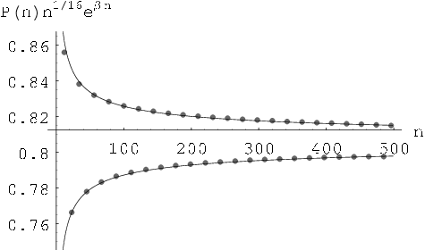
The amplitude of the oscillations is

$\displaystyle A_{1}(\gamma)$	$\displaystyle\equiv$	$\displaystyle{1\over\sqrt{2}}\;{G\left({1\over 4}\right)G\left({7\over 4}\right)\over G\left({3\over 4}\right)G\left({5\over 4}\right)}\;{\tau_{+}(0)\tau_{-}(\pi)\over\tau_{-}(0)\tau_{+}(\pi)}$	(3.70)
	$\displaystyle=$	$\displaystyle{1\over\sqrt{2}}\;{\Gamma\left({3\over 4}\right)\over\Gamma\left({1\over 4}\right)}\;{\tau(0)\over\tau(\pi)}\left({\tau_{-}(\pi)\over\tau_{-}(0)}\right)^{2}$
	$\displaystyle=$	$\displaystyle{\Gamma\left({3\over 4}\right)\over\Gamma\left({1\over 4}\right)}\;{1\over\gamma}\;\exp\left(4\lim_{\epsilon\rightarrow 0}\oint{{\displaystyle\rm\mathstrut d}z\over 2\pi}{\log\tau(z)\over z^{2}-(1+\epsilon)^{2}}\right),$

where we used (B.11) and the identity

G(z+1)=\Gamma(z)G(z).

(3.71)

To calculate the integral we deform the contour of integration as in Fig. 3.4e and find

A_{1}(\gamma)={\Gamma\left({3\over 4}\right)\over\Gamma\left({1\over 4}\right)}\;{1\over\sqrt{2\gamma}}.

(3.72)

We conclude that at $h=1$ the EFP decays exponentially at $n\to\infty$ but with an additional power law pre-factor and a damped oscillatory component.

Remark. It is curious to notice that the exponents $1/16$ and $9/16$ in (3.63) and (3.67) remind us of the scaling dimensions of spins $\sigma^{x}$ and $\sigma^{y}$ . ³³ 3 See Ref. [31] or (2.43,2.45), where it was shown that the power laws for the $\sigma^{x}$ and $\sigma^{y}$ correlators are $1/4$ and $9/4$ respectively. It looks as if the EFP operator (3.1), among other things, has inserted square roots of spins transverse to the magnetic field at the ends of the string.

3.3.2.2 $\Omega_{-}$ ( $h=-1$ )

For $h=-1$ the generating function $\sigma(q)$ does not vanish but has a phase discontinuity of $\pi$ at $q=\pi$ . We parametrize $\sigma(q)$ as

\sigma(q)=\tau^{1}(q){\rm e}^{-{{\rm i}\over 4}[(q-\pi){\rm\>mod\>}2\pi-\pi]}

(3.73)

and apply FH to obtain

P(n)\sim{\it E^{1}_{-1}(\gamma)}\>n^{-{1\over 16}}\>{\rm e}^{-\beta(-1,\gamma)n}

(3.74)

with

{\it E^{1}_{-1}}(\gamma)\equiv E[\tau]G\left({3\over 4}\right)G\left({5\over 4}\right){\tau_{-}^{1/4}(\pi)\over\tau_{+}^{1/4}(\pi))},

(3.75)

where $\beta(-1,\gamma)$ and $E[\tau]$ are defined in (3.37) and (3.46) with

\hat{\tau}_{k}=\hat{\sigma}_{k}+{(-1)^{k}\over 4k}\;\theta(k)-{(-1)^{k}\over 4k}\;\theta(-k)

(3.76)

and $\hat{\sigma}_{k}$ from (3.42).

We can stretch the gFH the same way as in the previous section for $h=+1$ by considering the second parametrization

\sigma(q)=\tau^{2}(q){\rm e}^{{\rm i}{3\over 4}[(q-\pi){\rm\>mod\>}2\pi-\pi]}

(3.77)

which gives

P^{\prime}(n)\sim{\it E^{2}_{-1}(\gamma)}\>n^{-{9\over 16}}\>{\rm e}^{-\beta(-1,\gamma)n}

(3.78)

with

{\it E^{2}_{-1}}(\gamma)\equiv E[\tau]G\left({1\over 4}\right)G\left({7\over 4}\right){\tau_{+}^{3/4}(\pi)\over\tau_{-}^{3/4}(\pi))}.

(3.79)

Adding this subleading term to (3.74) we obtain

P(n)\sim{\it E^{1}_{-1}}(\gamma)\>n^{-{1\over 16}}\left[1+A_{-1}(\gamma)/n^{1\over 2}\right]\>{\rm e}^{-n\beta(-1,\gamma)}

(3.80)

with

	$\displaystyle A_{-1}(\gamma)$	$\displaystyle\equiv$	$\displaystyle{G\left({1\over 4}\right)G\left({7\over 4}\right)\over G\left({3\over 4}\right)G\left({5\over 4}\right)}\;{\tau_{+}(\pi)\over\tau_{-}(\pi)}$		(3.81)
		$\displaystyle=$	$\displaystyle{\Gamma\left({3\over 4}\right)\over\Gamma\left({1\over 4}\right)}\;{\tau_{+}(\pi)\over\tau_{-}(\pi)}.$		(3.81)

We propose (3.80) as an asymptotic form for EFP at $h=-1$ .

3.4 The line $\Gamma_{E}$ : an exact calculation

Before we conclude our analysis of the EFP with the study of the isotropic XY model, let us check our results (3.40,3.12) on the special line⁴⁴ 4 We are grateful to Fabian Essler who suggested us to check our results on this special line and pointed out the reference [34] to us. in the phase diagram defined by

h^{2}+\gamma^{2}=1.

(3.82)

It was shown in Ref. [34] that on this line the ground state is a product of single spin states and is given by

|G\rangle=\prod_{j}|\theta,j\rangle=\prod_{j}\left[\cos\left({\theta\over 2}\right)|\uparrow,j\rangle+(-1)^{j}\sin\left({\theta\over 2}\right)|\downarrow,j\rangle\right],

(3.83)

where $|\uparrow,j\rangle$ is an up-spin state at the lattice site $j$ , etc. One can directly check that the state (3.83) is an eigenstate of (2.1) if the value of parameter $\theta$ is

\cos^{2}\theta=\frac{1-\gamma}{1+\gamma}

(3.84)

and (3.82) is satisfied. It is also easy to show [34] that this state is, in fact, the ground state of (2.1).

The probability of formation of a ferromagnetic string in the state (3.83) is obviously

P(n)=\sin^{2n}\left({\theta\over 2}\right)=\left({1\over 2}-{1\over 2}{h\over|h|}\sqrt{1-\gamma\over{1+\gamma}}\right)^{n},

(3.85)

which is an exact result on the line (3.82). The value of $\beta(h,\gamma)$ which immediately follows from this exact result is

\beta(h=\pm\sqrt{1-\gamma^{2}},\gamma)=-\log\left({1\over 2}\mp{1\over 2}\sqrt{1-\gamma\over{1+\gamma}}\right)=-\Lambda(h,\gamma),

(3.86)

where $\Lambda(h,\gamma)$ was defined in (3.19).

This is, indeed, consistent with (3.23) since under the condition (3.82) the function $\Delta(h,\gamma)$ vanishes. The integral (3.20) defining $\Delta(h,\gamma)$ vanishes for (3.82) because the branching points (3.16) and (3.17) collapse to the same point and therefore the region of integration shrinks to just one point (3.20). In fact, the Toeplitz matrix (3.8) generated by (3.9) becomes triangular on the line (3.82) with diagonal matrix element $(S_{n})_{jj}=\sin^{2}(\theta/2)$ and the determinant of ${\bf S_{n}}$ is exactly (3.85).

From the definitions of $\beta(h,\gamma)$ , we see that the decay factor consists of two terms, which now have a clear physical meaning. The $\Lambda(h,\gamma)$ term is the factor we found above in (3.86) and represents the contribution given by un-entangled spins. The remaining part accounts for the correlations between spins. Both $\Delta(h,\gamma)$ and the correlation functions given by (2.22) and (2.23) vanish on the line (3.82).

Finally, it should be noted that there are actually two ground states for the theory on this special line:

	$\displaystyle\|G_{+}\rangle$	$\displaystyle=$	$\displaystyle\prod_{j}\|\theta,j\rangle=\prod_{j}\left[\cos\left({\theta\over 2}\right)\|\uparrow,j\rangle+(-1)^{j}\sin\left({\theta\over 2}\right)\|\downarrow,j\rangle\right]$		(3.87)
	$\displaystyle\|G_{-}\rangle$	$\displaystyle=$	$\displaystyle\prod_{j}\|\theta,j\rangle=\prod_{j}\left[\cos\left({\theta\over 2}\right)\|\uparrow,j\rangle-(-1)^{j}\sin\left({\theta\over 2}\right)\|\downarrow,j\rangle\right]$		(3.88)

These two states break the translational symmetry and are orthogonal in the thermodynamic limit. The reason for this degeneracy of the ground state is yet not well understood.

If we were to consider a linear combination of these states, any local operator (involving only a finite number of lattice sites) would have vanishing cross-terms and very likely the same expectation value on either state (though one can design an operator which would violate the latter property). Therefore, for our present interest, evaluation of the EFP on any combination of these two ground states would yield the same result (3.85) and we don’t need to concern ourselves with this degeneracy.

The existence of these two ground states is instead of great interest in the study of quantum information applied to the XY model. We recently noticed this degeneracy and this helped us understand a previously known formula on the entropy of a block of neighboring spins [35]. This entropy is known to quantify the degree of entanglement of two subsystems of a system (in this case the block of neighboring spins and the rest of the chain). We remark in passing that many of the approaches to the calculation of the entropy for the XY model use Toeplitz determinant representations and the theory on Toeplitz determinant for deriving their asymptotic behavior, in the spirit of the present work.

3.5 The critical line $\Omega_{0}$ ( $\gamma=0$ ) and the Gaussian behavior

The case $\gamma=0$ , corresponding to the Isotropic XY Model, has been studied in Ref. [24]. For $\gamma=0$ the generating function (3.9) is reduced to the one found in [24].

For $|h|<1$ , the generating function $\sigma(q)$ has a limited support between $[-\cos^{-1}h,\cos^{-1}h]$ . To find the asymptotic behavior of the determinant of the Toeplitz matrix one can apply Widom’s Theorem [38] and obtain [24]

P(n)\sim 2^{5\over 24}{\rm e}^{3\zeta^{\prime}(-1)}(1-h)^{-{1\over 8}}n^{-{1\over 4}}\left({1+h\over 2}\right)^{n^{2}\over 2}.

(3.89)

We see that in this case, the EFP decays as a Gaussian with an additional power-law pre-factor.

In a different context, the formula (3.89) appeared also in [36] as a probability of forming a gap in the spectrum of unitary random matrices. This is not unexpected, since the joint eigenvalue distribution of unitary random matrices is known to coincide with the distribution of free fermions in the ground state.

For $|h|>1$ , the theory is no longer critical and the ground state is completely polarized in the $z$ direction, giving a trivial EFP $P(n)=0$ for $h>1$ and $P(n)=1$ for $h<-1$ .

3.6 Crossover between Gaussian and exponential behavior: a Bosonization approach

In order to understand qualitatively the crossover between the Gaussian asymptotic behavior at $\gamma=0$ and the exponential decay for $\gamma\neq 0$ , we employ a bosonization approach similar to the one used in [23], which will be sketched in Chapter 5. In the limit $\gamma\ll 1$ we consider the continuum limit of (2.7), bosonize the fermionic fields, and write the Euclidean action of the theory as ${\cal S}=\int{\displaystyle\rm\mathstrut d}x\,{\displaystyle\rm\mathstrut d}\tau{\cal L}$ , where $\tau\equiv{\rm i}t$ is the imaginary time and the Lagrangian is

{\cal L}={1\over 2}\left[\left(\partial_{\mu}\vartheta\right)^{2}-{2\gamma\over\pi}\cos\left(\sqrt{4\pi}\vartheta\right)\right],

(3.90)

where we also rescaled the time $\tau\to v_{F}\tau$ , with $v_{F}\equiv 2\sqrt{1-h^{2}}$ , the Fermi velocity at $\gamma=0$ .

This is a Sine-Gordon theory for the “conjugate field” $\vartheta(x,\tau)$ , which describes the imaginary time dynamics of our 1-D system. In terms of $\vartheta$ the density of fermions is given by $\rho={1\over\sqrt{\pi}}\partial_{\tau}\vartheta+\rho_{0}$ , where $\rho_{0}=k_{F}/\pi$ is the density of fermions in the ground state.

In the field theory approach, the EFP (see Ref. [23]) in the limit $n\to\infty$ would be given with exponential accuracy by the probability of an instanton $P(n)\sim e^{-{\cal S}_{0}}$ , where ${\cal S}_{0}$ is the action of the instanton. Here the instanton is the solution of the classical equations of motion of (3.90) which corresponds to the formation of an emptiness of length $n$ at the time $\tau=0$ . Unfortunately, the EFP instanton involves large deviations of the density of fermions from the equilibrium density $\rho_{0}$ and is beyond the bosonization approach as the derivation of (3.90) relies on the linearization of the fermionic spectrum near the Fermi points.

Following [23], we are going to slightly generalize our problem by considering the depletion formation probability instead of the EFP requiring

\left.\rho\right|_{\tau=0,\;0<x<n}=\rho_{0}+{1\over\sqrt{\pi}}\left.\partial_{\tau}\vartheta(x,\tau)\right|_{\tau=0,\;0<x<n}=\rho_{0}-\bar{\rho},

(3.91)

where $\bar{\rho}$ is some constant. The original EFP problem corresponds to $\bar{\rho}=\rho_{0}$ . Here, instead, we consider the probability of weak depletion, i.e.

-{1\over\sqrt{\pi}}\left.\partial_{\tau}\vartheta(x,\tau)\right|_{\tau=0,\;0<x<n}=\bar{\rho}<<\rho_{0}.

(3.92)

We study the latter using an instanton approach to (3.90) and infer the (qualitative) behavior of the original EFP from this weak limit.

To simplify the problem further, we assume that the instanton configuration is completely confined to one of the wells of the Cosine potential in (3.90) and that the field $\vartheta$ is small enough to allow for an expansion of the Cosine:

{\cal S}\approx{1\over 2}\int{\displaystyle\rm\mathstrut d}x\;{\displaystyle\rm\mathstrut d}\tau\left[\left(\partial_{\mu}\vartheta\right)^{2}+4\gamma\;\vartheta^{2}\right].

(3.93)

In this formulation, the anisotropy parameter $\gamma^{1/2}$ plays the role of the mass of the bosonized theory. The probability we are looking for is given by the action ${\cal S}_{0}$ of the classical field configuration which satisfies the Euler-Lagrange equation (in this case a Klein-Gordon equation in two dimensions) with the boundary condition (3.91)

P_{\bar{\rho}}(n)={\rm e}^{-{\cal S}_{0}}.

(3.94)

In the limit $\gamma=0$ , the theory is massless and scale invariant. In [23] it was shown that, due to the scale invariance, the action of the instanton is quadratic in $n$ . The instanton configuration in this case is essentially a droplet of depletion in space-time with dimensions proportional to $n$ both in the space and time direction, in order to satisfy the boundary condition (3.91). This result is consistent with the Gaussian asymptotic behavior prescribed by Widom’s theorem (see Sec. 3.5).

In the massive case, a finite correlation length $\xi\sim\gamma^{-1/2}$ is generated and we observe a crossover. For string lengths $n$ smaller than the correlation length $\gamma^{-1/2}$ , the instanton action is not sensitive to the presence of the finite correlation length and is still quadratic in $n$ (giving a Gaussian decay for EFP). In the asymptotic limit of string lengths greater than $\gamma^{-1/2}$ , the time dimension of a depletion droplet is of the order of $\xi$ (instead of $n$ as in the massless limit): the action is linear in $n$ and the probability has an exponential behavior.⁵⁵ 5 This picture is very similar to the one for massless theory at finite temperature. In the latter the inverse temperature plays the role of the correlation length [23] (see 3.7).

Figure 3.7: Plot of the value of the stationary action

{\cal S}_{0}

vs. the string length

n

. The action

{\cal S}_{0}

is obtained from (3.103) with

f(y)

given by the numerical solution of the singular integral equation (3.101). The graph depicts

{\cal S}_{0}(n)

for

m=2\sqrt{\gamma}=0.01

\bar{\rho}=0.2

. The crossover takes place around

n\sim 2/m=\sqrt{1/\gamma}=200

Figure 3.8: Plot of the derivative

d{\cal S}_{0}/dn

with

{\cal S}_{0}

from (3.103). The plot corresponds to

m=0.01

\bar{\rho}=0.2

and clearly shows a crossover from the quadratic to the linear behavior at

n\sim 2/m=\sqrt{1/\gamma}=200

In the next section we show how to solve the integral equation corresponding to the boundary problem (3.91,3.93) and present its numerical solution and some analytical results. Figures 3.8 and 3.8 clearly show the crossover between a quadratic behavior of the stationary action for small $n$ to a linear asymptotic one for $n\to\infty$ .

3.7 Calculation of the stationary action in the bosonization approach

In the previous section we have formulated the XY model near $\gamma=0$ in terms of the bosonic field with Lagrangian (3.93). It was also pointed out that, instead of the EFP, we are interested in the Probability of Formation of Weakly Ferromagnetic Strings (PFWFS) and that we are going to calculate this probability in the saddle point approximation. In this section we are going to show how to solve the integral equation that solves this problem.

This is a fairly technical section and can be easily skipped if the reader is not interested in the mathematical techniques required to tackle this problem.

We consider a configuration of the field (instanton) which satisfies the boundary condition imposed by the PFWFS (3.91,3.92)

\left.\partial_{\tau}\vartheta(x,\tau)\right|_{\tau=0,0<x<n}=\sqrt{\pi}\bar{\rho}

(3.95)

and that minimizes the action, i.e. that satisfies the Euler-Lagrange equations:

\left(\partial_{\mu}\partial^{\mu}-m^{2}\right)\vartheta=0.

(3.96)

The latter equation is the Klein-Gordon equation with the mass given by $m^{2}\equiv 4\gamma$ (see (3.93)). The PFWFS will be found from the value of the action ${\cal S}_{0}$ corresponding to this instanton configuration (3.94). In this appendix we calculate the stationary action needed in Sec. 3.6.

We now solve the differential equation (3.96) with non-trivial boundary condition (3.95) by recasting it as the integral equation:

\vartheta(x,\tau)={1\over 2\pi}\int_{0}^{n}\partial_{t}K_{0}\left(m\sqrt{(x-y)^{2}+\tau^{2}}\right)f(y)\;{\displaystyle\rm\mathstrut d}y,

(3.97)

where $K_{0}(x,x^{\prime};\tau,\tau^{\prime})$ is the modified Bessel function of 0-th order – the kernel of the differential operator (3.96) in two dimensions. We impose the boundary condition (3.95) by requiring that the “source” $f(y)$ satisfies

$\displaystyle\left.\partial_{\tau}\vartheta(x,0)\right\|_{0<x<n}$	$\displaystyle=$	$\displaystyle\lim_{\tau\to 0}{1\over 2\pi}\int_{0}^{n}\left\{K_{2}\left(m\sqrt{(x-y)^{2}+\tau^{2}}\right){m^{2}\tau^{2}\over(x-y)^{2}+\tau^{2}}\right.$	(3.98)
		$\displaystyle\quad\left.-\,K_{1}\left(m\sqrt{(x-y)^{2}+\tau^{2}}\right){m\over\sqrt{(x-y)^{2}+\tau^{2}}}\right\}f(y)\;{\displaystyle\rm\mathstrut d}y$
	$\displaystyle=$	$\displaystyle\sqrt{\pi}\bar{\rho}.$

This is the integral equation on $f(y)$ we have to solve.

Once the limit $\tau\to 0$ is taken, the kernel in Eq. (3.98) is singular. We isolate the singularity by rewriting equation (3.98) as:

{{\displaystyle\rm\mathstrut d}\over{\displaystyle\rm\mathstrut d}x}\;{1\over\pi}\;\mathchoice{{\vbox{\hbox{$\textstyle-$}}\kern-4.86108pt}}{{\vbox{\hbox{$\scriptstyle-$}}\kern-3.43057pt}}{{\vbox{\hbox{$\scriptscriptstyle-$}}\kern-2.908pt}}{{\vbox{\hbox{$\scriptscriptstyle-$}}\kern-2.76045pt}}\!\int_{0}^{n}{f(y)\over x-y}\;{\displaystyle\rm\mathstrut d}y+\lim_{\tau\to 0}\;{1\over\pi}\int_{0}^{n}G_{0}(x,\tau;y)f(y)\;{\displaystyle\rm\mathstrut d}y=2\sqrt{\pi}\bar{\rho}

(3.99)

with

	$\displaystyle G_{0}(x,\tau;y)$	$\displaystyle\equiv$	$\displaystyle{(x-y)^{2}-\tau^{2}\over(x-y)^{2}+\tau^{2}}+K_{2}\left(m\sqrt{(x-y)^{2}+\tau^{2}}\right){m^{2}\tau^{2}\over(x-y)^{2}+\tau^{2}}$		(3.100)
			$\displaystyle-K_{1}\left(m\sqrt{(x-y)^{2}+\tau^{2}}\right){m\over\sqrt{(x-y)^{2}+\tau^{2}}}$		(3.100)

or, after integration over $x$ , as

{1\over\pi}\;\mathchoice{{\vbox{\hbox{$\textstyle-$}}\kern-4.86108pt}}{{\vbox{\hbox{$\scriptstyle-$}}\kern-3.43057pt}}{{\vbox{\hbox{$\scriptscriptstyle-$}}\kern-2.908pt}}{{\vbox{\hbox{$\scriptscriptstyle-$}}\kern-2.76045pt}}\!\int_{0}^{n}{f(y)\over x-y}\;{\displaystyle\rm\mathstrut d}y+{1\over\pi}\int_{0}^{n}G(x;y)f(y)\;{\displaystyle\rm\mathstrut d}y=2\sqrt{\pi}\bar{\rho}\;x

(3.101)

with

G(x;y)\equiv\lim_{\tau\to 0}\int_{0}^{x}G_{0}(x_{1},\tau;y)\;{\displaystyle\rm\mathstrut d}x_{1}.

(3.102)

We have recasted Eq. (3.98) in the standard form for a singular integral equation (3.101). Once we have the solution of this equation, we can calculate the action corresponding to this instanton as

{\cal S}_{0}={\sqrt{\pi}\bar{\rho}\over 2}\int_{0}^{n}f(y)\;{\displaystyle\rm\mathstrut d}y.

(3.103)

We solved the singular integral equation (3.101) numerically and we computed the corresponding action (3.103). The results of this calculation are presented as a plot of the action ${\cal S}_{0}$ vs. $n$ in Fig. 3.8, where we notice the crossover from a quadratic to a linear behavior (corresponding to a crossover from Gaussian to exponential behavior for the probability, (3.94)) as we expected. To confirm the nature of this crossover, in Fig. 3.8 we plot $d{\cal S}_{0}/dn$ and we see that it starts linearly and then saturates asymptotically as it should.

In the limit $n\ll 1/m$ , we can expand the Bessel functions in the kernel (3.100)

G_{0}(x,\tau;y)=-{m^{2}\over 2}\left({\tau^{2}\over(x-y)^{2}+\tau^{2}}+{1\over 2}\ln\left[(x-y)^{2}+\tau^{2}\right]+\ln{m\over 2}+G-{1\over 2}\right)+\ldots,

(3.104)

where $G$ is Catalan’s constant. Then we solve the singular integral equation (3.101) to first order by first transforming it into a regular integral equation.

In [39], Chap. 14, Sec. 114 it is explained that a singular integral equation like (3.101) is equivalent to

f(x)+{1\over\pi{\rm i}}\int_{0}^{n}N(x;y)\;f(y)\;{\displaystyle\rm\mathstrut d}y=2\bar{\rho}\sqrt{\pi x(n-x)},

(3.105)

where the new kernel is

N(x;y)\equiv{\sqrt{x(n-x)}\over\pi{\rm i}}\;\mathchoice{{\vbox{\hbox{$\textstyle-$}}\kern-4.86108pt}}{{\vbox{\hbox{$\scriptstyle-$}}\kern-3.43057pt}}{{\vbox{\hbox{$\scriptscriptstyle-$}}\kern-2.908pt}}{{\vbox{\hbox{$\scriptscriptstyle-$}}\kern-2.76045pt}}\!\int_{0}^{n}{G(y^{\prime};y)\over\sqrt{y^{\prime}(n-y^{\prime})}(x-y^{\prime})}\;{\displaystyle\rm\mathstrut d}y^{\prime}.

(3.106)

Using (3.104), we can explicitly calculate the integral defining $N(x;y)$ in terms of elementary functions and after some algebra the integral equation (3.105) results in a long, but essentially simple, regular integral equation. Its solution is

	$\displaystyle f(x)$	$\displaystyle=$	$\displaystyle\sqrt{\pi}\bar{\rho}\left[2+{m^{2}n^{2}\over 8}\left(\ln{m\,n\over 8}+G-{3\over 2}\right)\right]\sqrt{x(n-x)}$		(3.107)
			$\displaystyle\quad-\sqrt{\pi}\bar{\rho}\;{m^{2}n^{2}\over 4}\left(x-{n\over 2}\right)\tan^{-1}\sqrt{x\over n-x}.$		(3.107)

The corresponding stationary action (3.103) is

{\cal S}_{0}=n^{2}\>{\pi^{2}\bar{\rho}^{2}\over 8}\left[1+{m^{2}n^{2}\over 16}\left(\ln{m\;n\over 8}+G-2\right)\right].

(3.108)

The first term in (3.108) corresponds to the Gaussian decay of PFWFS we expect in the limit of $m=0$ . In Fig. 3.9, we compare this analytical result for the action with the numerical result of Fig.3.8. In the plot, we include the pure Gaussian decay (the first term in (3.108)), which already gives a remarkable agreement for small $n$ . The full solution (3.108) extends this agreement further for larger $n$ . For $m=0$ ( $\gamma=0$ ), (3.108) reproduces the result calculated in [23] for $h=0$ .

3.8 Emptiness Formation Probability at finite temperature

Finally, we consider what happens at finite temperature ( $T>0$ ). The correlators (2.22) and (2.23) become

	$\displaystyle F_{jk}^{T}$	$\displaystyle\equiv$	$\displaystyle{\rm i}\langle\psi_{j}\psi_{k}\rangle_{T}=-{\rm i}\langle\psi_{j}^{\dagger}\psi_{k}^{\dagger}\rangle_{T}=\int_{0}^{2\pi}{{\displaystyle\rm\mathstrut d}q\over 2\pi}{1\over 2}\sin\vartheta_{q}\tanh{\varepsilon_{q}\over 2T}{\rm e}^{{\rm i}q(j-k)},$
	$\displaystyle G_{jk}^{T}$	$\displaystyle\equiv$	$\displaystyle\langle\psi_{j}\psi_{k}^{\dagger}\rangle_{T}=\int_{0}^{2\pi}{{\displaystyle\rm\mathstrut d}q\over 2\pi}{1\over 2}\left(1+\cos\vartheta_{q}\tanh{\varepsilon_{q}\over 2T}\right){\rm e}^{{\rm i}q(j-k)},$		(3.109)

where the additional factor takes care of the thermal average.

The EFP is expressed by

P(n)\equiv{1\over Z}\mbox{Tr}\,\left\{{\rm e}^{-\frac{H}{T}}\prod_{j=1}^{n}{1-\sigma_{i}^{z}\over 2}\right\},

(3.110)

and in the spinless fermion formalism it becomes

P(n)=\langle\prod_{i=1}^{n}\psi_{i}\psi_{i}^{\dagger}\rangle_{T}.

(3.111)

We again use Wick’s Theorem (or its thermal version, called Bloch-de Dominicis theorem [40]) to express it as a Pfaffian. The calculation proceeds the same way as for zero temperature and the EFP can be represented as

P(n)=|\det({\bf T_{n}})|,

(3.112)

where ${\bf T_{n}}$ is the $n\times n$ Toeplitz matrix generated by the function

t(q)={1\over 2}\left(1+{\rm e}^{{\rm i}\vartheta_{q}}\tanh{\varepsilon_{q}\over 2T}\right),

(3.113)

where the “rotation angle” $\vartheta_{q}$ and the spectrum $\varepsilon_{q}$ were defined in (2.9) and (2.11) respectively.

The generating function $t(q)$ is never-vanishing and has zero winding number. Therefore, for $T>0$ we can apply the standard Szegö Theorem to obtain

P(n){\stackrel{{\scriptstyle n\rightarrow\infty}}{{\sim}}}E(h,\gamma,T){\rm e}^{-n\beta(h,\gamma,T)},

(3.114)

where

$\displaystyle\beta(h,\gamma,T)$	$\displaystyle=$	$\displaystyle-\int_{0}^{2\pi}{{\displaystyle\rm\mathstrut d}q\over 2\pi}\;\log\left\|t(q)\right\|$	(3.115)
	$\displaystyle=$	$\displaystyle-{1\over 2}\int_{0}^{2\pi}{{\displaystyle\rm\mathstrut d}q\over 2\pi}\;\log\left[{1\over 2}\left(1+{\cos q-h\over\varepsilon_{q}}\tanh{\varepsilon_{q}\over 2T}\right)\right],$	(3.115)
$\displaystyle E(h,\gamma,T)$	$\displaystyle=$	$\displaystyle\exp\left(\sum_{k=1}^{\infty}k\hat{t}_{k}\hat{t}_{-k}\right)$	(3.116)

with

\hat{t}_{k}=\int_{0}^{2\pi}{{\displaystyle\rm\mathstrut d}q\over 2\pi}{\rm e}^{-{\rm i}kq}\log\left[{1\over 2}\left(1+{\cos q-h+{\rm i}\gamma\sin q\over\varepsilon_{q}}\tanh{\varepsilon_{q}\over 2T}\right)\right],

(3.117)

and $\varepsilon_{q}$ is given as in (2.11) by

\varepsilon_{q}=\sqrt{(\cos q-h)^{2}+\gamma^{2}\sin^{2}q}.

(3.118)

As can be expected from simple thermodynamic considerations, at finite temperature the behavior is always purely exponential asymptotically. As it was shown in [23], at finite but very low temperatures one can observe a crossover from the zero temperature behavior at short string lengths $n$ to the exponential behavior (3.114) in the limit of very large $n$ . This crossover occurs at a length scale of the order of the inverse temperature.

EFP for the Anisotropic XY model
Region	$\gamma$ , $h$	$P(n)$	Eq.	Section	Theorem
$\Sigma_{-}$	$h<-1$	$E\,{\rm e}^{-n\beta}$	3.40	3.3.1.1	Szegö
$\Sigma_{0}$	$-1<h<1$	$E\,{\rm e}^{-n\beta}$	3.40	3.3.1.2	FH
$\Sigma_{+}$	$h>1$	${\it E}\left[1+(-1)^{n}A\right]\>{\rm e}^{-n\beta}$	3.54	3.3.1.3	gFH
$\Gamma_{E}$	$\gamma^{2}+h^{2}=1$	$E\,{\rm e}^{-n\beta}$	3.85	3.4	Exact
${\bf\Omega_{+}}$	$h=1$	${\it E}\>n^{-{1/16}}\left[1+(-1)^{n}A/\sqrt{n}\>\right]\>{\rm e}^{-n\beta}$	3.69	3.3.2.1	gFH
${\bf\Omega_{-}}$	$h=-1$	${\it E}\>n^{-{1/16}}\left[1+A/\sqrt{n}\>\right]\>{\rm e}^{-n\beta}$	3.80	3.3.2.2	gFH
${\bf\Omega_{0}}$	$\gamma=0$ , $\|h\|<1$	$E\,n^{-1/4}e^{-n^{2}\alpha}$	3.89	3.5	Widom

Table 3.1: Asymptotic behavior of the EFP in different regimes. The exponential decay rate

\beta

is given by Eq. (3.12) for all regimes. The regions in boldface are the critical ones. The coefficients

E,A

are functions of

h

and

\gamma

whose explicit expressions are provided in the text. Relevant theorems on Toeplitz determinants are collected in the B.

3.9 Discussion and conclusions

The asymptotic behavior of the Emptiness Formation Probability $P(n)$ as $n\to\infty$ for the Anisotropic XY model in a transverse magnetic field as a function of the anisotropy $\gamma$ and the magnetic field $h$ has been studied. We have summarized our results in Table 3.1. These asymptotic behaviors were first presented in [30].

Our main motivation has been to study the relation between the criticality of the theory and the asymptotics of the EFP. Let us now consider the results on the critical lines ( $\Omega_{0}$ and $\Omega_{\pm}$ in Fig. 2.1). The Gaussian behavior on $\Omega_{0}$ ( $\gamma=0$ , $|h|<1$ ) is in accord with the qualitative argument of Ref. [23] using a field theory approach. In $\Sigma_{0}$ ( $\gamma\neq 0$ , $|h|<1$ ) the asymptotic decay is exponential. We proposed a physical interpretation of the crossover between the two asymptotes using a bosonization analysis of the region of small $\gamma$ : we suggest that there is an intermediate regime of Gaussian decay for the string lengths smaller than $1/\sqrt{\gamma}$ which crosses over to the exponential behavior for longer strings.

On the critical lines $\Omega_{\pm}$ , the decay of the EFP is exponential instead of Gaussian, and apparently contradicts the qualitative picture of Ref. [23]. The reason for this disagreement is that although at $h=\pm 1$ the model can be rewritten in terms of massless quasiparticles $\chi$ defined in (2.8), we are still interested in the EFP for the “original” Jordan-Wigner fermions $\psi$ . In terms of $\chi$ this correlator has a complicated (nonlocal) expression very much different from the simple one (3.2). From the technical point of view, the difference is that in the qualitative argument in favor of a Gaussian decay of EFP for critical systems there is an implicit assumption that the density of fermions (or magnetization) is related in a local way to the field responsible for the critical degrees of freedom (free boson field $\phi$ ). This assumption is not valid on the lines $h=\pm 1$ . The theory is critical on those lines and can be described by some free field $\phi$ . However, the relation between the magnetization and this field is highly nonlocal and one can not apply the simple argument of [23] to the XY model at $h=\pm 1$ .

Although EFP at the critical magnetic field does not show a Gaussian behavior, there is an important difference between the asymptotic behavior of EFP on and off critical lines. Namely, a power-law pre-factor $n^{-\lambda}$ appears on all critical lines. For the XY model it is universal (i.e. $\lambda$ is constant on a given critical line) and takes values $\lambda=1/4$ for $\gamma=0$ [24] and $\lambda=1/16$ on the lines $h=\pm 1$ . It would be interesting to understand which operators determine these particular “scaling dimensions” of the EFP (see the remark at the end of Section 3.3.2.1).

At $h\geq 1$ the use of gFH predicts even-odd oscillations of $P(n)$ . We compared the predicted oscillations to numerical calculations of Toeplitz determinants and found a very good agreement (see Figs. 3.5,3.6). We proposed a physical interpretation of the oscillations as coming from pair correlations of spins which can be clearly seen as superconducting correlations in the fermionic representation (2.6).

In some parts of the phase diagram ( $\Sigma_{+}$ , $\Omega_{\pm}$ ) we used the so-called generalized Fisher-Hartwig conjecture [37] which is not yet proven. However, our numeric calculations support the analytical results (see Figures 3.5 and 3.6). We note that to the best of our knowledge this is the first physically motivated example where the original Fisher-Hartwig conjecture fails and its extended version is necessary. ⁶⁶ 6 We note that recently the theory on Toeplitz determinants has been used and extended with new results in order to calculate yet one more important physical quantity. We refer the interested reader to [41], [42] and [43], where the entanglement for the XY Spin chain and for Random matrix models have been calculated. We also suggest that the gFH could be used to find the subleading corrections to the asymptotic behavior, as we did for $h=\pm 1$ in (3.69,3.80). This novel hypothesis is supported by our numerics and it would be interesting to confirm it analytically.

In conclusion, we notice that it was straightforward to generalize our results for nonzero temperature. The only modification is that at $T\neq 0$ the thermal correlation functions must be used instead of (2.22,2.23). Then, the generating function (3.9) is non-singular everywhere and we have an exponential decay of $P(n)$ in the whole phase diagram according to the standard Szegö Theorem and standard statistical mechanics arguments. We presented results for $T\neq 0$ in Section 3.8.

Chapter 4 The Hydrodynamic Approach

Very often it is possible to treat a quantum many body system as a continuum. A description of this kind views the system as a fluid, where the motion of the individual particles is not important, but one is interested in their collective behavior. This idea has a long history (see [17, 44, 45, 19] for instance).

We consider a one-dimensional system at zero temperature, in the thermodynamic limit. We will take a “semi-classical” limit, bringing Planck’s constant $\hbar$ to zero and the number of particles $N$ to infinity in such a way that their product stays constant. This limit allows us to describe the system only in terms of its local density and velocity.

These two fields are clearly not sufficient to describe all states of the whole system, but they will provide an accurate approximation of it for some sectors of the theory. For instance we cannot consider configurations where the particles occupy disconnected regions of the phase-space (see Figure 4.2).

The hydrodynamic approach can be applied to exactly integrable systems, where the description in terms of just two fields is essentially exact, once we limit our attention to the ‘allowed’ sectors of the theory.

The traditional hydrodynamic approach developed in the 1960’s [44] addresses finite temperature systems and studies the time evolution of conserved quantities in many particle models. We concentrate instead on zero-temperature dynamics.

The conservation laws guarantee that a perturbation or a fluctuation in the density of a conserved quantity of the system will not disappear on a length scale of the order of the interparticle distance, but will diffuse on a macroscopic length scale. The diffusion equation is the main dynamical equation describing the evolution of these quantities. This description relies heavily on non-equilibrium processes taking place at a microscopical level to average into a diffusive motion. Once the dynamical equation is established, it is relatively simple to calculate some asymptotics of correlation functions for the conserved quantities using statistical mechanics methods.

It is clear from this brief explanation that the hydrodynamic description is valid in the long wavelength approximation, with wavelengths longer than any other length scale of the system, so that diffusion averages have meaning and one can use the continuum description of the system.

We are taking a zero temperature limit, where quantum fluctuations take the role of thermal fluctuations.

Hydrodynamic equations are non-linear differential equations and their solution and treatment is not easy. If one linearizes them, the resulting theory is what is known in studying one-dimensional models as “Bosonization”. Bosonization is a renowned tool, with a long history, to calculate correlators for the strongly interacting one dimensional systems. However, there are phenomena which cannot be captured by a linearized theory. For instance the calculation of the Emptiness Formation Probability is beyond the linear approximation. In the next chapter we show how one can calculate the EFP to leading order for a number of systems using the hydrodynamic approach.

Before we can analyze any system in particular, in section 4.1 we introduce some definitions and show the basic structure of the quantities of interest. Then, in Section 4.2 we start explaining our approach on the example of the simplest possible system: Free Fermions (FF). This will allow us to warm up slowly to Section 4.3 where we generalize the approach to other systems with a derivation based on a Lagrangian Formalism. In section 4.4 we show how a linearized hydrodynamics reduces to the standard bosonization.

Finally, in section 4.5 we show how the Bethe Ansatz technique can be used to derive the hydrodynamic Hamiltonian of an integrable system. The Bethe Ansatz allows one to calculate exactly, although implicitly, the wavefunctions of an integrable system. Even more importantly, it provides fundamental information on the thermodynamics of the theory and an easier access to the conserved quantities of the model. For a short summary of the Bethe Ansatz, we refer the reader to Appendix C.

In Appendix D we show that if we neglect gradient corrections in a Galilean invariant system, the resulting hydrodynamic theory possesses a double infinite series of conserved quantities. It is still unclear whether these conserved quantities are enough to make the theory integrable in the sense of Liouville (i.e. the phase-space can be exactly factorized into a series of tori described by the action-angle variables). The answer is probably negative. But what is even more puzzling is the underlying symmetry guaranteeing this abundance of conserved quantities and its physical meaning. We suggest that origin of this quantities should be connected to that of free fermions system, but we are unable to prove this conjecture at this moment.

Zero temperature hydrodynamics was first developed by Landau in [17]. The collective description approach was successfully used in the context of lower-dimensional string theories and two-dimensional quantum gravity [46]. Our treatment is based on the work of A.G. Abanov and collaborators and it was described in [19].

4.1 Some preliminaries

Let us start by introducing some definitions.

We want to develop a hydrodynamic description of a system in terms of its local density

\rho(x)\equiv\sum_{j=1}^{N}m\delta(x-x_{j})

(4.1)

and current

	$\displaystyle j(x)$	$\displaystyle\equiv$	$\displaystyle{1\over 2}\sum_{j=1}^{N}\left\{p_{j},\delta(x-x_{j})\right\}$		(4.2)
		$\displaystyle=$	$\displaystyle-{\rm i}{\hbar\over 2}\sum_{j=1}^{N}\left\{{\partial\over\partial x_{j}},\delta(x-x_{j})\right\},$		(4.2)

where the sums are performed over the positions $x_{j}$ of every particle in the system and

\left\{A,B\right\}\equiv A\cdot B+B\cdot A

(4.3)

is the anti-commutator. The velocity is then defined as

v\equiv{1\over 2}\left({1\over\rho}j+j{1\over\rho}\right).

(4.4)

From this point onward we will always intend the velocity and current to be properly symmetrized, but we will not write it explicitly for the sake of brevity (e.g. (4.4) will be written as $v=j/\rho$ ).

In a Hamiltonian formalism the dynamics of the system is encoded in the Hamiltonian (expressed as a function of the hydrodynamic parameters $\rho$ and $v$ ) and in the commutation relation between $\rho$ and $v$ .

A “natural” assumption for the form of a hydrodynamic Hamiltonian is

H=\int\rho(x){\displaystyle\rm\mathstrut d}x\left[m{v^{2}(x)\over 2}+\epsilon\left(\rho(x)\right)\right],

(4.5)

where $\epsilon(\rho)$ is the internal energy per particle as a function of the local density of particles. The integration measure is equivalent to a sum over all particles, while the first term is the traditional macroscopic kinetic term. The second term in the Hamiltonian is some sort of potential term that includes all the interaction, but also the effect of the quantum statistics. We are going to see that this form is indeed the correct one in the next sections.

A very important point is how we take the thermodynamic limit. We are going to see later that the internal energy $\epsilon(\rho)$ is often an essentially quantum quantity, which vanishes in the classical limit ( $\hbar\to 0$ ). In such case, we are interested in taking the number of particles to infinity in a way that the internal energy stays finite as $\rho\to\infty$ and $\hbar\to 0$ . We are going to show how to derive the Hamiltonian for different systems in the next sections.

Assuming standard commutation relation between position and momentum,

[x_{i},p_{j}]\equiv x_{i}p_{j}-p_{j}x_{i}={\rm i}\hbar\delta_{ij},

(4.6)

from their microscopical definitions (4.1,4.2) we can calculate

\left[\rho(x),j(y)\right]={\rm i}\hbar\rho(y)\partial_{x}\delta(x-y)

(4.7)

or, using (4.4),

\left[\rho(x),v(y)\right]=-{\rm i}\hbar\delta^{\prime}(x-y),

(4.8)

where $\delta^{\prime}(x)$ denotes the derivative of the Dirac’s delta-function. Eq. (4.8) is the canonical commutation relation for hydrodynamic parameters (see, for instance, [47]) and, in connection with the Hamiltonian of the system (4.5), will specify the time evolution of $\rho$ and $v$ :

$\displaystyle\rho_{t}$	$\displaystyle=$	$\displaystyle{{\rm i}\over\hbar}[H,\rho]$	(4.9)
	$\displaystyle=$	$\displaystyle-\partial_{x}(\rho\,v),$	(4.9)
$\displaystyle v_{t}$	$\displaystyle=$	$\displaystyle{{\rm i}\over\hbar}[H,v]$	(4.10)
	$\displaystyle=$	$\displaystyle-\partial_{x}\left({v^{2}\over 2}+(\rho\epsilon)_{\rho}\right).$	(4.10)

4.2 The simplest example: Free Fermions

Let us consider a one dimensional system of Free Fermions (FF), without internal degrees of freedom. The local density of particles is given by

\rho(x)=m\int{{\displaystyle\rm\mathstrut d}k\over 2\pi\hbar}.

(4.11)

Let us assume that the system moves with some velocity $v(x)$ , which itself is a slow function of $x$ . This means that the left and right Fermi points are also functions of $x$ so that:

\rho(x)=m\int_{k_{L}(x)}^{k_{R}(x)}{{\displaystyle\rm\mathstrut d}k\over 2\pi\hbar}=m{k_{R}(x)-k_{L}(x)\over 2\pi\hbar}.

(4.12)

The momentum density of the system is then given by

P(x)\equiv j(x)=\int_{k_{L}(x)}^{k_{R}(x)}k\;{{\displaystyle\rm\mathstrut d}k\over 2\pi\hbar}={k^{2}_{R}(x)-k^{2}_{L}(x)\over 4\pi\hbar},

(4.13)

where we recognized that the momentum of the system is in fact its current

j(x)=\rho(x)\;v(x).

(4.14)

From this equation and using (4.12,4.13), we express the local velocity of the system as

v(x)={k_{R}(x)+k_{L}(x)\over 2m}.

(4.15)

Equations (4.12,4.15) give us the hydrodynamic parameters of the free fermions fluid $\rho$ and $v$ in terms of the left and right Fermi points $k_{L,R}$ .

We invert (4.12,4.15) and get the right and left Fermi momenta as functions of the density and velocity at each point in space and time:

k_{R,L}(x,t)=m\;v(x,t)\pm{\hbar\pi\over m}\;\rho(x,t).

(4.16)

This is one of the most important limitations of our approach. For the Fermi points to be functions of the coordinates, they have to be single valued. This means that we can only describe star-like configurations (a.k.a. quadratic profiles) that in phase-space look like in Figure 4.1. We cannot address states similar to the one in Figure 4.2, where disconnected regions of phase-space are populated or where the world-line of $k_{R,L}$ goes back above or below itself.

The Hamiltonian of a free fermions system is

H=\int_{k_{L}}^{k_{R}}{k^{2}\over 2m}\;{{\displaystyle\rm\mathstrut d}k\over 2\pi\hbar}={k^{3}_{R}-k^{3}_{L}\over 12\pi\hbar m}

(4.17)

and, by using (4.16), can be written in terms of the density and velocity of the system as

E(x)=H={\rho(x)v^{2}(x)\over 2}+{\hbar^{2}\pi^{2}\over 6m^{4}}\rho^{3}(x).

(4.18)

We are now in a position to discuss what kind of thermodynamic limit we are interested in. As we increase the number of particles, we let the density grow as well. As we approach the semi-classical limit with $\hbar\to 0$ , we let the density grow so that the product of the two quantity remains constant:

\hbar\rho\to{\rm const}

(4.19)

This means that the energy per particle remains finite and that the kinetic and potential terms (respectively the first and the second term in (4.18)) have comparable magnitude. To make this point more apparent, let us rescale the velocity as

v\to{m\over\hbar}\;v

(4.20)

so that the Hamiltonian becomes

H={\hbar^{2}\over m^{2}}\left({\rho v^{2}\over 2}+{\pi^{2}\over 6m^{2}}\rho^{3}\right).

(4.21)

From this point on, we will set constants $\hbar=m=1$ , this means that all quantities are going to be expressed in units of $\hbar$ and $m$ :

H(x)={\rho(x)v^{2}(x)\over 2}+{\pi^{2}\over 6}\rho^{3}(x).

(4.22)

Note that the second term on the right hand side gives the internal energy of the system as $\epsilon(\rho)={\pi^{2}\over 6}\rho^{2}$ and that this contribution comes only from the Pauli principle, since we are describing free fermions. For this reason it is not correct to identify the internal energy with a pure potential term.

We showed in the previous section that the microscopic description of the system (4.1,4.2,4.4) imposes the following commutation relation between density and velocity:

\left[\rho(x),v(y)\right]=-{\rm i}\delta^{\prime}(x-y).

(4.23)

Using this relation, the Hamilton equations give us the dynamics of the system:

	$\displaystyle\rho_{t}(x)=\left[H(x),\rho(y)\right]$	$\displaystyle=$	$\displaystyle-\partial_{x}(\rho v),$
	$\displaystyle v_{t}(x)=\left[H(x),v(y)\right]$	$\displaystyle=$	$\displaystyle-\partial_{x}\left({v^{2}\over 2}+{\pi^{2}\over 2}\rho^{2}\right).$		(4.24)

We recognize the first equation as the continuity equation that expresses particle conservation and relates density and velocity of the system as dependent quantities

\partial_{t}\rho+\partial_{x}(\rho v)=0.

(4.25)

The second dynamical equation is:

\partial_{t}v+v\partial_{x}v=-\pi^{2}\rho\partial_{x}\rho

(4.26)

and is known as the “Euler equation” in the classical theory of fluids.

We have shown in the simple case of free fermions how to construct a collective description of the system in terms of local density and velocity, which represents its hydrodynamic description.

It is worth noticing here that we derived (4.25,4.26) essentially semi-classically. For the free fermion case (and only for this case), it can be shown [46] that a quantum treatment of the theory gives exactly the same results, i.e. one only needs to consider commutation relations instead of Poisson bracket, all the functions are promoted to be operators (we put “hats” on top of the density, velocity and Hamiltonian) and all equations have to be interpreted as operator equations.

In the next section we generalize this construction to some interacting systems.

4.3 Lagrangian formulation of Hydrodynamics

As we showed in section 3.6, the leading behavior of the EFP can be easily calculated in the semiclassical approximation. To this end it is useful now to turn to a Lagrangian formalism to calculate the hydrodynamic action and the partition function of the quantum theory [19].

We consider the partition function

Z=\int{\cal D}u\;{\rm e}^{{\rm i}{\cal S}[u]},

(4.27)

where ${\cal S}[u]$ is the Action

{\cal S}[u]=\int{\displaystyle\rm\mathstrut d}x\int{\displaystyle\rm\mathstrut d}t{\cal L}(u,\dot{u})

(4.28)

of some field or collection of fields $u(x,t)$ and where $\dot{u}\equiv\partial_{t}u$ .

Eventually, in the next chapter, we are interested in calculating the EFP as a rare fluctuation in the equilibrium configuration, an “instanton”, and this configuration will take place in imaginary time. To do this, we will need to formulate the Euclidean theory with the Euclidean action

{\cal S}_{E}[u]=\int{\displaystyle\rm\mathstrut d}x\int_{-1/2T}^{1/2T}{\displaystyle\rm\mathstrut d}\tau{\cal L}(u,\partial_{\tau}u),

(4.29)

with periodic boundary conditions in the imaginary time $\tau={\rm i}t$ defined by the temperature of system $T$ .

Let us first consider a system with Galilean invariance¹¹ 1 Lattice systems are more complicated and have not been treated in this thesis for lack of time, but their analysis will be addressed shortly.. The requirement of Galilean invariance restricts considerably the form of the lagrangian to

{\cal L}(\rho,v)={\rho v^{2}\over 2}+\rho\epsilon(\rho)+\ldots

(4.30)

where the first term is the kinetic energy of the system and is the only one that can depend on the velocity and the second term is the internal energy of the fluid, to be determined by the fluid’s equation of state. $\epsilon(\rho)$ is the internal energy per particle at given density $\rho$ . Other terms can be included in the lagrangian and were here denoted by the dots: these terms include spatial derivatives of density and velocity and can be neglected if density and velocity gradients are sufficiently small.

Particle conservation requires the continuity equation

\partial_{t}\rho+\partial_{x}j=0

(4.31)

to be satisfied, where $j=\rho v$ . We can interpret this equation as a constraint on the fields, relating $\rho$ and $v$ to each other. We can solve this constraint by introducing the “particle displacement field” $u(x,t)$ such that

	$\displaystyle\rho$	$\displaystyle\equiv$	$\displaystyle\rho_{0}+\partial_{x}u,$
	$\displaystyle j$	$\displaystyle\equiv$	$\displaystyle-\partial_{t}u,$		(4.32)

where $\rho_{0}$ is the equilibrium value of the density at infinity, so that the displacement field can satisfy standard boundary conditions and vanish at infinity. (One could define the displacement field in terms of the microscopic theory like in (4.1,4.2) as

u(x)\equiv\sum_{j=1}^{N}\theta(x-x_{j})-\rho_{0}x

(4.33)

where the sum is over the $x_{j}$ position of all particles in the system and $\theta(x)$ is the Heaviside Step-function.)

One can then write the Lagrangian in terms of the displacement field:

{\cal L}(u,\dot{u})={\dot{u}^{2}\over 2(\rho_{0}+u_{x})}+(\rho_{0}+u_{x})\epsilon(\rho_{0}+u_{x})

(4.34)

and look for the field configuration minimizing the action ${\cal S}[u]$ . We can write the Euler-Lagrange equation for this Lagrangian in terms of the physical field:

\partial_{t}v+v\partial_{x}v=-\partial_{x}\partial_{\rho}\left[\rho\epsilon(\rho)\right],

(4.35)

where $\rho$ and $v$ were defined in terms of $u(x,t)$ in 4.32. This is the Euler equation for a one dimensional fluid [47] and reduces to (4.26) for the free fermions case ( $\epsilon(\rho)={\pi^{2}\over 6}\rho^{2}$ ).

We see that, once the internal energy $\epsilon(\rho)$ in (4.30) is known from the equation of state, one has everything to calculate the Lagrangian of a one-dimensional Galilean invariant system. In section 4.5 we are going to show how to compute the internal energy $\epsilon(\rho)$ as a function of the density for integrable models, using the Bethe Ansatz solution. Alternatively, for non-integrable systems one can compute $\epsilon(\rho)$ from numerics or from other phenomenological methods.

The problem is not equally straightforward for systems without Galilean invariance, like for lattice models. Nonetheless, a hydrodynamic description can be developed in such cases as well. In chapter 6 we will consider systems with more than one type of particles, namely fermions with spin, and their hydrodynamics will not be as simple as the one for Galilean invariant models.

4.4 Bosonization as a linearized hydrodynamics

If the deviations from the equilibrium state are small, we can expand the Lagrangian (4.34) around $\rho=\rho_{0}$ and $j=0$ as

{\cal L}(u,\dot{u})\sim{1\over 2\rho_{0}}\left(\dot{u}^{2}+v_{s0}^{2}\,u_{x}^{2}\right),

(4.36)

where we defined the sound velocity at equilibrium as

v_{s0}^{2}\equiv\rho\left.\partial_{\rho}^{2}\left(\rho\epsilon(\rho)\right)\right|_{\rho=\rho_{0}}.

(4.37)

By scaling the time as $v_{s0}t\to t$ we can write the linearized Action as

{\cal S}\sim{v_{s0}\over\rho_{0}}\int{\displaystyle\rm\mathstrut d}^{2}x{1\over 2}\left(\partial_{\mu}u\right)^{2},

(4.38)

where ${\displaystyle\rm\mathstrut d}^{2}x\equiv{\displaystyle\rm\mathstrut d}x{\displaystyle\rm\mathstrut d}t$ and $\mu=x,t$ .

The linearized hydrodynamics is described by the familiar quadratic action of bosonization, giving the Laplace equation

\Delta u=0

(4.39)

as the equation of motion.

4.5 Hydrodynamics from the Bethe Ansatz

The Bethe Ansatz is a powerful tool to analyze integrable systems. For the reader unfamiliar with this technique, we review in Appendix C the basic formulas that we need to develop our hydrodynamic approach. In fact, once one is familiar with the machinery, its use in the hydrodynamic formalism is quite straightforward.

The Bethe Ansatz solution is based on the distribution of the quasi-momenta $\tau(q)$ . This distribution is found as the solution of an integral equation known as the Bethe Equation (C.23):

\tau(q)+\int_{-k}^{k}K(q-q^{\prime})\tau(q^{\prime}){\displaystyle\rm\mathstrut d}q^{\prime}={1\over 2\pi},

(4.40)

where the Kernel $K(q-q^{\prime})$ encodes the interactions of the system.

For the ground state of the system, the limits of integration in the integral equation are chosen to be symmetric, i.e. from $-k$ to $k$ . But we are interested in a different sector of the theory, a sector characterized by a total finite momentum of the system²² 2 One can think as the ground state of the theory as coming from a grand-canonical ensemble approach. One then constructs the partition function by adding to the Hamiltonian a vector potential coupled to the total momentum of the theory, in addition to the standard chemical potential coupled to the number of particles..

We are guided by our experience with the free fermions model in section 4.2³³ 3 One can derive the free fermions case from the general formalism we are developing in this section using the Bethe Ansatz. One has just to keep in mind that for free fermions, the kernel in (4.40) is equal to zero, therefore the momentum distribution is $\tau=1/2\pi$ . and we assume asymmetric limits of integration for the Bethe equation:

\tau(q)+\int_{k_{L}}^{k_{R}}K(q-q^{\prime})\tau(q^{\prime}){\displaystyle\rm\mathstrut d}q^{\prime}={1\over 2\pi}.

(4.41)

The number of particles and momentum per unit length of the system are given by (C.25,C.26). If we assume them to be space dependent, we can identify them as the density and current we need for our hydrodynamic description:

	$\displaystyle\rho(x)$	$\displaystyle=$	$\displaystyle\int_{k_{L}(x)}^{k_{R}(x)}\tau(q){\displaystyle\rm\mathstrut d}q,$		(4.42)
	$\displaystyle j(x)$	$\displaystyle=$	$\displaystyle\int_{k_{L}(x)}^{k_{R}(x)}q\;\tau(q){\displaystyle\rm\mathstrut d}q.$		(4.43)

The energy of the system is given by

H(x)=\int_{k_{L}(x)}^{k_{R}(x)}{q^{2}\over 2}\tau(q){\displaystyle\rm\mathstrut d}q.

(4.44)

This is an implicit expression for the Hamiltonian, since it depends on the momentum density $\tau(q)$ , which in turn is a function of $k_{R}$ and $k_{L}$ .

We could invert (4.42,4.43) and express $k_{R}$ and $k_{L}$ as a function of $\rho$ and $j$ (as we did for the free fermions) and then use this relation to express the Hamiltonian as a function of the hydrodynamic parameters density and current.

We can actually do better. For a system like this we can use Galilean invariance to boost the reference frame. In practice, we perform a change of variable in the integrations by shifting the integration variable as

q^{\prime}=q-v

(4.45)

where

v\equiv{k_{R}+k_{L}\over 2}

(4.46)

so that equations (4.42,4.43) become

	$\displaystyle\rho(x)$	$\displaystyle=$	$\displaystyle\int_{-k(x)}^{k(x)}\tau^{\prime}(q^{\prime}){\displaystyle\rm\mathstrut d}q^{\prime}$		(4.47)
	$\displaystyle j(x)$	$\displaystyle=$	$\displaystyle\int_{-k(x)}^{+k(x)}(q^{\prime}+v)\;\tau^{\prime}(q^{\prime}){\displaystyle\rm\mathstrut d}q^{\prime}=\rho(x)v(x)$		(4.48)

where we use the fact the the function $\tau^{\prime}(q^{\prime})=\tau(q+v)$ is even and where

k={k_{L}-k_{R}\over 2}.

(4.49)

More importantly, this change of variable writes the Hamiltonian as

	$\displaystyle H$	$\displaystyle=$	$\displaystyle{\rho v^{2}\over 2}+\int_{-k}^{k}{q^{\prime 2}\over 2}\tau^{\prime}(q^{\prime}){\displaystyle\rm\mathstrut d}q^{\prime}$		(4.50)
		$\displaystyle=$	$\displaystyle{\rho v^{2}\over 2}+\rho\epsilon(\rho)$		(4.50)

where

\epsilon(\rho)\equiv{1\over\rho}\int_{-k}^{k}{q^{\prime 2}\over 2}\tau^{\prime}(q^{\prime}){\displaystyle\rm\mathstrut d}q^{\prime}.

(4.51)

This is precisely the expression we derived in generality in (4.5) or (4.30), but now we have a microscopic way to calculate the internal energy function $\epsilon(\rho)$ , from the Bethe Ansatz. Moreover, the formalism developed in this section will prove very powerful when applied to more complicated systems as we are going to see in Chapter 6.

To conclude, we recall once more that from the commutation relation (4.8) and using (4.9,4.10), we get the equations of motion (4.31,4.35).

Chapter 5 The EFP from Hydrodynamics

We now turn back to the problem of calculating the correlator known as Emptiness Formation Probability. In Chapter 3 we calculated the asymptotics of this correlation function in the XY model. This calculation was facilitated by the specific structure of the model which allowed us to express the EFP exactly as the determinant of a matrix.

We argued in Chapter 1 for the importance of the EFP in the theory of integrable models. There, we also pointed out that the EFP can provide us with important insights in the general problem of calculating correlators that involve large deviations from the equilibrium configuration. We propose the hydrodynamic approach to address this problem.

We introduced our hydrodynamic approach in the previous chapter; here we are going to show how this formalism helps us in calculating the leading asymptotic behavior of the EFP for some integrable models possessing a simple Galilean invariance.

We are going to calculate the EFP as the probability of a rare fluctuation of the theory, an “instanton” which depletes a region of particles.

In section 5.1 we are going to explain how we are setting up the calculation and draw some general conclusion. In section 5.2 we are going to attempt the calculation using the linearized hydrodynamics (also know as Bosonization) and show that this approximation is only enough to produce the correct qualitative, but not quantitative result. In section 5.3 we are going to manipulate the action of the theory to show that we can extract the leading behavior of the EFP from the asymptotic behavior of the instanton solution. In section 5.4 we are going to use this result to calculate the EFP for the free fermions hydrodynamics we constructed in section 4.2. Then, in section 5.5 we will consider Calogero-Sutherland particles and calculate the EFP in the hydrodynamic approach.

These results were presented for the first time in [19]. In the next chapters we are going to develop a hydrodynamic description for more complicated models and we will show for the first time how to calculate the EFP for these models.

5.1 EFP as an instanton configuration

We consider the Lagrangian formulation of the hydrodynamic theory introduced in section 4.3. We are going to work in Euclidean space, i.e. in imaginary time, because we are not studying the dynamical evolution of the system, but a property of the ground state.

We write the action of the Euclidean hydrodynamic theory as

Z=\int{\cal D}u\;e^{-{\cal S}_{E}[u]},

(5.1)

where ${\cal S}_{E}[u]$ was defined in (4.29).

Our approach is essentially the same as the one used in section 3.6. The asymptotic behavior of the EFP is defined as a rare fluctuation that depletes a region of length $2R$ from every particle. We interpret this configuration $u(\tau,x)$ as the result of a collective motion where all particles move away so that at some time $\tau=0$ we have no particles in the spatial interval $\left[-R,R\right]$ .

This trajectory $u(\tau,x)$ is a solution of the equations of motion satisfying the EFP boundary conditions:

\rho(\tau=0;-R<x<R)=0,

(5.2)

and standard boundary conditions at infinity

	$\displaystyle\rho$	$\displaystyle\to$	$\displaystyle\rho_{0},\;\;\;\;x,\tau\to\infty,$
	$\displaystyle v$	$\displaystyle\to$	$\displaystyle 0,\;\;\;\;x,\tau\to\infty,$		(5.3)

Then with exponential accuracy, the EFP is calculated as

P(R)\sim e^{-{\cal S}_{opt}},

(5.4)

where ${\cal S}_{opt}$ is the value of the action (4.29) on the configuration $u(x,t)$ .

In the introduction of Chapter 3 we already argued that we can estimate the qualitative dependence on $R$ of the stationary action ${\cal S}_{opt}$ on very general grounds. The argument went as follows: in order to satisfy the EFP boundary conditions 5.2, the instanton solution needs to open a gap in its density that perturbs the configuration both in space and time. The spatial extent of this disturbance is clearly of the order of the gap to be opened, i.e. $R$ .

If we assume that the effective fluid we are describing is compressible and there are no other relevant length scales in the system, then the typical time scale of the disturbance has to be of the order of $R/v_{s}$ , where $v_{s}$ is the sound velocity at $\rho=\rho_{0}$ . Therefore, the (space-time) “area” of the disturbance is of the order of $R^{2}$ , the action ${\cal S}_{opt}\sim R^{2}$ and we conclude that the decay of the EFP (5.4) is going to be Gaussian:

P(R)\sim e^{-\alpha R^{2}},

(5.5)

where $\alpha$ is some (non-universal) constant depending on the details of (4.29).

In general, this behavior will persist until another length scale emerges to compete with $R$ . At finite but sufficiently low temperatures, the temporal extent of the instanton $R/v_{s}$ is smaller than the inverse temperature $R/v_{s}\ll 1/T$ and the instanton does not feel the effect of the temperature, resulting in am intermediate Gaussian decay of EFP as in (5.5). However, as the temperature increases, or as we consider bigger $R$ , the periodic boundary conditions in time become relevant and the $1/T$ scale defines the temporal size of the instanton, so that the space-time area of the disturbance scales as $R$ and one obtains

P(R)\sim e^{-\gamma R}.

(5.6)

Similarly, if some other term in the theory (4.29) drives the system away from criticality, the hydrodynamic approach will describe an incompressible fluid. The correlation length of the density fluctuations will have the same effect of a relevant length scale as just discussed and the EFP will decay exponentially as in (5.6) even at zero temperature if $R$ is bigger than this correlation length. In both cases, as one increases $R$ , one would observe a crossover from Gaussian to exponential behavior, with the crossover happening when $R\sim v_{s}\over T$ or then $R$ is comparable with the relevant correlation length.

Once again, this is the same argument of [23] and we have shown the latter crossover phenomenon in (3.6).

Before we proceed to any actual calculation, for the sake of generality, we would like to consider a slightly different problem from the Emptiness Formation Probability (5.2). We are going to impose the Depletion Formation Probability (DFP) conditions on the instanton configuration:

\rho(\tau=0;-R<x<R)=\bar{\rho},

(5.7)

where $\bar{\rho}$ is some constant density. Setting $\bar{\rho}=0$ we obtain the EFP problem while for $\bar{\rho}$ close to $\rho_{0}$ one can use the bosonization technique to calculate $P(R;\bar{\rho})$ .

In conclusion, we would like to find a solution to the equations of motion that satisfy the boundary conditions (5.7,5.3) and then use this solution to calculate the value of the stationary action ${\cal S}_{opt}$ . In Euclidean space, due to the different sign convention, the Euler equation is

\partial_{\tau}v+v\partial_{x}v=\partial_{x}\partial_{\rho}[\rho\epsilon(\rho)],

(5.8)

and the continuity equation reads

\partial_{\tau}\rho+\partial_{x}j=0.

(5.9)

5.2 Linearized hydrodynamics or bosonization

A simple qualitative analysis would tell us why we cannot calculate the EFP using a bosonization approach. In fact, one of the most important approximations done in deriving the bosonization description of a system is to assume a linear spectrum. This is definitely a very reasonable assumption when one wants to look at low energy excitations close to the Fermi points, but the EFP clearly picks up contributions from every point in the spectrum, since it imposes a strong deviation from the equilibrium distribution in the configuration space. As we pointed out in Chapter 1, the inability of Bosonization to describe the EFP is one of the main motivations for our study of this correlator, since it is a poster child of the advantage of using a hydrodynamic description over bosonization for certain calculations.

However, we can try to calculate the DFP (5.7) in the bosonization approach if

{\rho_{0}-\bar{\rho}\over\rho_{0}}\ll 1,

(5.10)

i.e., if we consider the probability of formation of a only small constant density depletion along the long string $-R<x<R$ .

In this case the deviation of the density from $\rho_{0}$ is small almost everywhere, as we will show below, and therefore we can assume that only particles close to the Fermi surface will be involved in the creation of the depletion and bosonization is applicable.

As we showed in section 4.4, we can derive bosonization by linearizing the hydrodynamic action (4.29) into (4.38). The corresponding linearized equation of motion for the displacement field $u(\tau,x)$ is the Laplace equation

\Delta u=0

(5.11)

which has to be solved with the DFP boundary condition

u(\tau=0,x)=-(\rho_{0}-\bar{\rho})x,\quad\mbox{for}\;-R<x<R.

(5.12)

In [19], this problem was solved by inspection and the correct instanton solution was found to be

u(x,t)=-(\rho_{0}-\bar{\rho})\,\Re\left(z_{0}-\sqrt{z_{0}^{2}-R^{2}}\right),

(5.13)

with the complex notation

z_{0}\equiv x+{\rm i}v_{s0}\tau

(5.14)

and where $v_{s0}$ was defined in (4.37) as

v_{s0}^{2}\equiv\rho\left.\partial_{\rho}^{2}\left(\rho\epsilon(\rho)\right)\right|_{\rho=\rho_{0}}.

(5.15)

One can check that indeed, at $\tau=0$ , $-R<x<R$ the complex coordinate $z_{0}$ is real and square root in (5.13) is purely imaginary so that (5.12) is satisfied. At space-time infinity $z_{0}\to\infty$ we have

u(x,t)\approx-{\alpha\over z_{0}}-{\bar{\alpha}\over\bar{z_{0}}}

(5.16)

with

\alpha=\bar{\alpha}\equiv{1\over 4}\left(\rho_{0}-\bar{\rho}\right)\,R^{2}

(5.17)

and where we used $\bar{z_{0}}\equiv x-{\rm i}v_{so}\tau$ to denote complex conjugation.

In terms of the original hydrodynamic parameters (4.32), we obtain from (5.16) that as $z_{0}\to\infty$

	$\displaystyle\rho$	$\displaystyle\approx$	$\displaystyle\rho_{0}+{\alpha\over z_{0}^{2}}+{\bar{\alpha}\over\bar{z_{0}^{2}}},$
	$\displaystyle v$	$\displaystyle\approx$	$\displaystyle-{\rm i}{v_{s0}\over\rho_{0}}\left({\alpha\over z_{0}^{2}}-{\bar{\alpha}\over\bar{z_{0}^{2}}}\right),$		(5.18)

which obviously satisfy the boundary conditions at infinity (5.3).

By plugging this instanton solution (5.13) into (4.38), we can calculate the stationary action for the DFP problem as

{\cal S}_{DFP}={1\over 2}{v_{s0}\over\pi\rho_{0}}\left[\pi(\rho_{0}-\bar{\rho})\,R\right]^{2}.

(5.19)

Let us end this section by noticing that the instanton solution (5.13) is singular close to the ends of the string $t=0$ , $x=\pm R$ and therefore gradients of $u$ , i.e. density and velocity, diverge. This is not consistent with our approximation justifying the bosonization approach, i.e. that the solution does not deviate too much from its equilibrium value. However, in [19] the corrections coming from those areas were estimated to contribute only with terms of higher order in the small parameter (5.10) to the action (5.19).

5.3 EFP through the asymptotics of the solution

In [19], Abanov showed that the calculation of the value of the stationary action $S_{opt}$ (5.4) can be extracted from the asymptotics of the EFP solution of the hydrodynamic equations, using a Maupertui principle.

The first step is to calculate the variation of the action (4.29) with respect to the displacement field $u$

	$\displaystyle\delta{\cal S}_{E}$	$\displaystyle=$	$\displaystyle\int{\displaystyle\rm\mathstrut d}^{2}x\,\Big\{-\partial_{\tau}(v\delta u)-\partial_{x}\left[\left({v^{2}\over 2}-\partial_{\rho}(\epsilon\rho)\right)\delta u\right]$		(5.20)
			$\displaystyle+\delta u\left[\partial_{\tau}v+v\partial_{x}v-\partial_{x}\partial_{\rho}(\epsilon\rho)\right]\Big\}.$		(5.20)

Note that we kept surface terms (full derivatives) in addition to the last term which produces the equation of motion (5.8).

Let us now calculate the derivative of the action ${\cal S}_{E}$ with respect to the equilibrium background density $\rho_{0}$ and evaluate it on the EFP (or DFP) solution that saturates the equations of motion:

\partial_{\rho_{0}}{\cal S}_{opt}=\int{\displaystyle\rm\mathstrut d}^{2}x\,\left\{-\partial_{\tau}(v\partial_{\rho_{0}}u)-\partial_{x}\left[\left({v^{2}\over 2}-\partial_{\rho}(\epsilon\rho)\right)\partial_{\rho_{0}}u\right]\right\}.

(5.21)

We can rewrite the full derivative terms in (5.21) as a boundary term

\displaystyle\partial_{\rho_{0}}{\cal S}_{opt}=\oint\,\left[v\partial_{\rho_{0}}u\,{\displaystyle\rm\mathstrut d}x+\left(\partial_{\rho}(\epsilon\rho)-{v^{2}\over 2}\right)\partial_{\rho_{0}}u\,{\displaystyle\rm\mathstrut d}\tau\right],

(5.22)

where the integral is taken over an infinitely large contour around the $x-\tau$ plane.

Equation (5.22) gives us the value of the (derivative of the) stationary action from boundary terms lying at infinitely large $x$ and $\tau$ . If we assume the asymptotic behavior for the instanton solution to be

$\displaystyle u(x,t)$	$\displaystyle\approx$	$\displaystyle-{\alpha\over z_{0}}-{\bar{\alpha}\over\bar{z}_{0}},$
$\displaystyle\rho$	$\displaystyle\approx$	$\displaystyle\rho_{0}+{\alpha\over z_{0}^{2}}+{\bar{\alpha}\over\bar{z}_{0}^{2}},$
$\displaystyle v$	$\displaystyle\approx$	$\displaystyle-{\rm i}{v_{s0}\over\rho_{0}}\left({\alpha\over z_{0}^{2}}-{\bar{\alpha}\over\bar{z}_{0}^{2}}\right),$	(5.23)

like in (5.16,5.18), after some algebra we conclude

\partial_{\rho_{0}}{\cal S}_{opt}=2\pi{v_{s0}\over\rho_{0}}(\alpha+\bar{\alpha}).

(5.24)

The problem of calculating the leading behavior of the EFP (DFP) is then reduced to the evaluation of the asymptotic behavior of the instanton solution. Once one knows $\alpha$ in (5.23), by integrating equation (5.24) one finds the desired behavior of the EFP (DFP) problem.

We can check this result with what we found in the previous section from bosonization. Substituting into (5.24) the value of $\alpha$ obtained in (5.17) we obtain

\partial_{\rho_{0}}{\cal S}_{opt}=\pi{v_{s0}\over\rho_{0}}(\rho_{0}-\bar{\rho})\,R^{2}

(5.25)

which is equivalent to (5.19) up to higher order terms in the small parameter (5.10).

5.4 EFP for Free Fermions

In section 4.2 we analyzed in details the hydrodynamic description of free fermions. The hydrodynamic equations for this system are

	$\displaystyle\partial_{\tau}\rho+\partial_{x}(\rho v)$	$\displaystyle=$	$\displaystyle 0,$
	$\displaystyle\partial_{\tau}v+v\partial_{x}v$	$\displaystyle=$	$\displaystyle\pi^{2}\rho\partial_{x}\rho.$		(5.26)

with the sound velocity

v_{s}=v_{F}=k_{F}=\sqrt{\rho\partial_{\rho}^{2}(\rho\epsilon)}=\pi\rho

(5.27)

where we noticed that, since in our notation $m=1$ , the sound velocity and Fermi velocity are the same for free fermions.

By introducing a complex field

w\equiv\pi\rho+{\rm i}v,

(5.28)

we can rewrite both dynamical equations (5.26) as the single complex Hopf equation²² 2 In real time formalism, instead of $w$ and $\bar{w}$ , one introduces right and left Fermi momenta $k_{R,L}=\pi\rho\pm v$ which satisfy the Euler-Hopf equations $\partial_{t}k+k\partial_{x}k=0$ , reflecting the absence of interactions between fermions.:

\partial_{\tau}w-{\rm i}w\partial_{x}w=0.

(5.29)

The general solution of this equation can be written implicitly as

w=F(x+{\rm i}w\tau)=F(z),

(5.30)

where $F(z)$ is an arbitrary analytic function of the complex variable $z$ defined as

z\equiv x+{\rm i}w\tau.

(5.31)

We can determine the function $F(z)$ through the boundary conditions. In [19] it was shown that by defining

F(z)\equiv\pi\bar{\rho}+\pi(\rho_{0}-\bar{\rho}){z\over\sqrt{z^{2}-R^{2}}}

(5.32)

equation (5.30) satisfies the DFP problem and we can get the EFP solution by setting $\bar{\rho}=0$ .

One obtains the density and velocity by taking the real and imaginary part of $w$ . To write down this instanton solution explicitly is quite complicated, since one has to solve the equation

w-\pi\bar{\rho}=\pi(\rho_{0}-\bar{\rho}){z\over\sqrt{z^{2}-R^{2}}}.

(5.33)

Abanov in [19] plotted a numerical solution that we show in figures 5.1 and 5.2).

However, as we argued in the previous section, to calculate the leading behavior of the EFP (DFP), we do not need to know the full solution of (5.33), but we just need the asymptotic behavior of the instanton solution using (5.24).

In the limit $x,\tau\to\infty$ we have $w\to\pi\rho_{0}$ and $z=x+{\rm i}w\tau\to x+{\rm i}\pi\rho_{0}\tau=z_{0}$ . Therefore, $w$ from (5.33) behaves asymptotically as

w-\pi\rho_{0}\approx\pi(\rho_{0}-\bar{\rho}){R^{2}\over 2z_{0}^{2}}

(5.34)

and taking, e.g., its real part we have

\rho-\rho_{0}\approx{1\over 4}(\rho_{0}-\bar{\rho})R^{2}\left({1\over z_{0}^{2}}+{1\over\bar{z}_{0}^{2}}\right).

(5.35)

Comparing (5.35) with (5.23) we identify

\alpha={1\over 4}(\rho_{0}-\bar{\rho})R^{2}.

(5.36)

Substituting this into (5.24) we find

\partial_{\rho_{0}}{\cal S}_{opt}=\pi^{2}(\rho_{0}-\bar{\rho})R^{2}

(5.37)

and, after integrating in $\rho_{0}$ ,

{\cal S}_{opt}={1\over 2}\left[\pi(\rho_{0}-\bar{\rho})R\right]^{2}.

(5.38)

We can conclude that DFP and EFP are respectively

	$\displaystyle P_{{\rm DFP}}(R)$	$\displaystyle\sim$	$\displaystyle\exp\left\{-{1\over 2}\left[\pi(\rho_{0}-\bar{\rho})\,R\right]^{2}\right\},$		(5.39)
	$\displaystyle P_{{\rm EFP}}(R)$	$\displaystyle\sim$	$\displaystyle\exp\left\{-{1\over 2}\left(\pi\rho_{0}\,R\right)^{2}\right\}.$		(5.40)

We can compare this result with the known results on the EFP for free fermions [36] that we recapitulated in Appendix A and confirm that (5.40) gives the correct first (Gaussian) term.

5.5 EFP for the Calogero-Sutherland model

Our final example for this chapter is the Calogero-Sutherland model, an integrable model of one-dimensional particles interacting with an inverse square potential. The Hamiltonian of the model is

	$\displaystyle H$	$\displaystyle=$	$\displaystyle-\frac{1}{2}\sum_{j=1}^{N}\frac{\partial^{2}}{\partial x_{j}^{2}}+\frac{1}{2}\sum_{1\leq j<k\leq N}\frac{\lambda(\lambda-1)}{(x_{j}-x_{k})^{2}}$		(5.41)
		$\displaystyle=$	$\displaystyle-\frac{1}{2}\sum_{i=1}^{N}\left(\frac{\partial}{\partial x_{i}}+\sum_{j=1,j\neq i}^{N}\frac{\lambda}{x_{i}-x_{j}}\right)\left(\frac{\partial}{\partial x_{i}}-\sum_{k=1,k\neq i}^{N}\frac{\lambda}{x_{i}-x_{k}}\right).$		(5.41)

and we are going to consider it in the thermodynamic limit $N\to\infty$ while keeping the density constant as we discussed in the previous chapter (4.19)³³ 3 Technically, in order to go into the thermodynamic limit, we need either to add an external harmonic potential to confine the particles or to consider the model as defined on a closed ring; otherwise the repulsive nature of the interaction would spread the particles and we would not be able to keep the density fixed. We can neglect these details here, since they do not change anything relevant for us and, most of all, they both preserve the integrability of the model..

This model is known to be integrable [48, 49] and we briefly analyzed it in the appendix dedicated to the Bethe Ansatz (C.8). We can write explicitly the ground state wavefunction of (5.41) as

\Psi_{GS}=\prod_{j<k}(x_{j}-x_{k})^{\lambda}.

(5.42)

As discussed in Appendix C, this formula shows that Calogero-Sutherland particles have intermediate statistics interpolating between non-interacting bosons ( $\lambda=0$ ) and non-interacting fermions ( $\lambda=1$ ).

As a connection to the theory of Random matrices we mentioned in 1.4, we should point out that that the probability distribution of particle coordinates

\left|\Psi_{GS}\right|^{2}=\prod_{j<k}|x_{j}-x_{k}|^{2\lambda}

(5.43)

at some particular values of the coupling constant $\lambda=1/2,\,1,\,2$ coincides with the joint probability of eigenvalues for the orthogonal, unitary, and symplectic random matrix ensembles respectively (see Eq. (1.7)).

To calculate the leading behavior of the EFP for the Calogero-Sutherland model we need to determine the equation of motion of its hydrodynamic description (5.8), which means that we need to know the internal energy function $\epsilon(\rho)$ . This can easily be found in [49] or from a direct Bethe Ansatz calculation and is

\epsilon(\rho)={\pi^{2}\over 6}\,\lambda^{2}\,\rho^{2}.

(5.44)

We immediately notice that (5.44) differs from the free fermion case ( $\epsilon_{FF}(\rho)={\pi^{2}\over 6}\,\rho^{2}$ ) just by a factor of $\lambda^{2}$ and coincides with the latter (as expected) at $\lambda=1$ .

Therefore, we can repeat the exact same analysis as in the last section and derive the EFP (DFP) very easily. Introducing the complex Riemann invariants

w\equiv\lambda\pi\rho+{\rm i}v

(5.45)

and repeating the calculations of the previous section we obtain

	$\displaystyle P_{{\rm DFP}}(R)$	$\displaystyle\sim$	$\displaystyle\exp\left\{-{1\over 2}\lambda\left[\pi(\rho_{0}-\bar{\rho})\,R\right]^{2}\right\},$		(5.46)
	$\displaystyle P_{{\rm EFP}}(R)$	$\displaystyle\sim$	$\displaystyle\exp\left\{-{1\over 2}\lambda\left(\pi\rho_{0}\,R\right)^{2}\right\}.$		(5.47)

Once again we can compare this result with what is already known(A.6) and confirming that, indeed, (5.47) gives the exact leading asymptotics of the EFP for the Calogero-Sutherland model. Subleading (in $1/R$ ) corrections to (5.47) are due to gradient corrections to the hydrodynamic action (5.44) and to quantum fluctuations around the found instanton which go beyond our accuracy.

Chapter 6 Hydrodynamics for a Spin-Charge System

One of the most interesting predictions of the Luttinger Liquid (LL) model is the effect known as the spin charge separation, according to which, in a one-dimensional system, the fundamental excitations are “holons” and “spinons” and they carry independently the charge and spin degrees of freedom of the electrons respectively.

These results of the LL model have been known for many years, but only now are we reaching the technological advancements necessary to test it experimentally. In recent years many laboratories have attempted to confirm this prediction (see, for instance [3]-[13]) and the data are definitely in accordance with the theory. What is still missing is a conclusive test that would firmly link the experimental results to the theoretical prediction, in that the methods used so far are fairly indirect and their interpretation is not unique.

While devices are developed right now to overcome this problem and confirm with certainty the occurrence of spin-charge separation in one dimension, we are interested in looking ahead and investigating the correction to this prediction.

In fact, it is well known that this effect is valid only for low energy excitations, in that its derivation assumes the spectrum to be linear. It is also known that the curvature of the spectrum will destroy perfect spin-charge separation for higher energy excitations and introduce a coupling between the spin and charge degrees of freedom.

Unfortunately, the field theory description underlying the LL model (bosonization), becomes inconsistent if one were to consider a non-linear spectrum: even a reasonable quadratic spectrum generates a theory with no stable vacuum. Even if one tries to perturbatively include corrections to the linear spectrum approximation, the expectation values calculated with this theory are divergent and to complete a reasonable bosonization calculation beyond the linear spectrum approximation is still an open challenge in many contexts.

To address the problem of determining the corrections to exact spin-charge separation we propose the hydrodynamic approach. We already discussed with the example of the EFP how the hydrodynamic approach is a natural generalization of a bosonization description to include the full spectrum of the microscopic theory. Therefore, we expect to be able to generalize the bosonization description of electrons in terms of non-interacting holons and spinons to include curvature corrections that will couple the two degrees of freedom.

This hydrodynamic description will involve two interacting fluids, one describing the bulk motion of the system, i.e. the charge, and one the internal degrees of freedom, i.e. the spin. In the limit of linear spectrum the interactions between these two fluids will vanish and one would recover traditional LL results, while normally the interactions will mix spin and charge in the fluids. Ideally, we might find that the gradient-less hydrodynamic description is integrable in the sense of Appendix D. Then, one could be able to derive the stable excitations of the system, “solitons”, i.e. one could identify two stable quasi-particles that would carry a fraction of the total charge and of the total spin of an electron each.

To derive the hydrodynamic description, we use the exactly solvable model of electrons with contact interactions, which was first solved using the Bethe Ansatz in [50]. Another interesting integrable model to consider would be the spin Calogero-Sutherland model [51], which can be solved using the asymptotic Bethe Ansatz. These two models are at opposite limits, in that one assumes the shortest interaction possible, i.e. contact interaction, while the other describes an inverse quadratic long range potential. While these can be good approximations to some physical systems, most systems lie in between these two extremes. Nonetheless, studying the limiting cases, where the theory of integrable models can help us, will allow us to us gain some insights on the general structure of a hydrodynamic description of spinful electrons.

In section 6.1 we sketch how one would bosonize a theory with quadratic spectrum and show that the resulting model has an unstable vacuum and that a perturbative treatment of the curvature of the spectrum generates divergences in the calculation of physical observables. In section 6.2, we describe the Bethe solution for a gas of electrons with contact interaction and we show how to implicitly derive its hydrodynamic description.

6.1 Bosonization for a quadratic spectrum

When one wants to construct the bosonization description of a system, the first step is to linearize the spectrum. As we are going to show, it is hard to make sense of the bosonization of a non-linear spectrum. Therefore, often one refers to “bosonization” as the whole procedure of linearizing the spectrum and then expressing the system in terms of its density excitations. However, it is important to keep in mind that in this section we are going to distinguish these two steps and call “bosonization” just the transformation from the microscopic degrees of freedom to the collective ones. In doing so we are aware that we are losing rigorousness and that the resulting model has to be interpreted carefully.

With these remarks in mind, let us now sketch how one would bosonize a quadratic theory. For simplicity, let us consider free fermions:

	$\displaystyle{\cal H}$	$\displaystyle=$	$\displaystyle-\Psi^{\dagger}(x)\partial_{x}^{2}\Psi(x)$		(6.1)
		$\displaystyle=$	$\displaystyle k^{2}\Psi^{\dagger}(k)\Psi(k)$		(6.1)

where $\partial_{x}\equiv\partial/\partial x$ and the second line shows the spectrum of the Hamiltonian in the Fourier space representation.

The traditional bosonization approach linearizes the spectrum as

	$\displaystyle{\cal H}$	$\displaystyle=$	$\displaystyle-\sum_{L,R}\psi^{\dagger}_{L,R}\left(\partial_{x}\pm{\rm i}k_{F}\right)^{2}\psi_{L,R}$		(6.2)
		$\displaystyle\simeq$	$\displaystyle-k_{F}^{2}\sum_{L,R}\psi^{\dagger}_{L,R}\psi_{L,R}\mp{\rm i}k_{F}\sum_{L,R}\psi^{\dagger}_{L,R}\partial_{x}\psi_{L,R}+\ldots$		(6.2)

where the first term is interpreted as a chemical potential and can be absorbed in a redefinition of the ground energy, while the second term expresses the linear spectrum of the excitations around the Fermi points $\pm k_{F}$ . Moreover, we defined left- and right-moving fields $\psi_{L,R}$ as the fields obtained expanding around the left/right Fermi Point:

\Psi(x)=:{\rm e}^{{\rm i}k_{F}x}\psi_{R}(x)+{\rm e}^{-{\rm i}k_{F}x}\psi_{L}(x):\;.

(6.3)

In bosonization one effectively describes the system with a single collective field that captures the density fluctuation. In practice, one makes the following transformation:

\psi_{L,R}(x)\equiv{1\over\sqrt{2\pi}}{\rm e}^{\pm{\rm i}\sqrt{4\pi}\phi_{L,R}(x)},

(6.4)

where $\phi_{L,R}$ are the left and right moving bosonic fields.

We use the transformation (6.4) to calculate various bilinears in the spin fields. For instance, one can consider a quantity like

	$\displaystyle:\psi_{L,R}^{\dagger}(x)\psi_{L,R}(x+\epsilon):$	$\displaystyle=$	$\displaystyle{1\over 2\pi}:{\rm e}^{\pm{\rm i}\sqrt{4\pi}\left(\phi_{L,R}(x+\epsilon)-\phi_{L,R}(x)\right)}:{\rm e}^{\pm 4\pi\langle\phi_{L,R}(x)\phi_{L,R}(x+\epsilon)\rangle}=$		(6.5)
		$\displaystyle=$	$\displaystyle{1\over 2{\rm i}\pi\epsilon}\left[{\rm e}^{\pm{\rm i}\sqrt{4\pi}\left(\phi_{L,R}(x+\epsilon)-\phi_{L,R}(x)\right)}-1\right]$		(6.5)

where we used the identity

{\rm e}^{A}{\rm e}^{B}=:{\rm e}^{A+B}:\;{\rm e}^{\langle AB+{A^{2}+B^{2}\over 2}\rangle}

(6.6)

and the fact that

\langle\psi_{L,R}(0)\psi_{L,R}(x)-\psi_{L,R}^{2}(0)\rangle=\lim_{\alpha\to 0}{1\over 4\pi}\ln{\alpha\over\alpha\pm{\rm i}x}.

(6.7)

The colons denote normal ordering¹¹ 1 Normal ordering means that in the evaluation we should put the creation operators to the right of all the annihilation operators. This convention is equivalent to subtracting un-physical zero energy contributions. and in the second line of (6.5) we used the fact the normal ordering simply amounts to subtract $1$ from the exponential.

We can expand (6.5) in powers of $\epsilon$ to find

	$\displaystyle:\psi_{L,R}^{\dagger}(x)\psi_{L,R}(x+\epsilon):$	$\displaystyle=$	$\displaystyle\sum_{n=0}^{\infty}{\epsilon^{n}\over n!}\psi_{L,R}^{\dagger}(x)\partial^{n}\psi_{L,R}(x)$		(6.8)
		$\displaystyle=$	$\displaystyle{1\over 2{\rm i}\pi\epsilon}\left[{\rm e}^{\pm{\rm i}\sqrt{4\pi}\sum_{n=1}^{\infty}{\epsilon^{n}\over n!}\phi_{L,R}^{(n)}(x)}-1\right]$		(6.8)

which give the generating function of the fermionic currents

j^{L,R}_{n}(x)\equiv\psi_{L,R}^{\dagger}(x)\partial_{L,R}^{n}\psi(x)

(6.9)

in terms of the bosonic field $\phi_{L,R}$ .

By matching powers of $\epsilon$ in (6.8) we can write down these expressions. The density of fermion is

\rho_{L,R}=j^{L,R}_{0}=\psi_{L,R}^{\dagger}(x)\psi_{L,R}(x)=\pm{1\over\sqrt{\pi}}\partial_{x}\phi_{L,R}(x),

(6.10)

the current density is

j^{L,R}_{1}=\psi_{L,R}^{\dagger}(x)\partial_{x}\psi_{L,R}(x)={\rm i}\left(\partial_{x}\phi_{L,R}(x)\right)^{2}\pm{1\over\sqrt{4\pi}}\partial_{x}^{2}\phi_{L,R}\;.

(6.11)

The third term in the expansion can be identify with the original quadratic Hamiltonian for the left/right movers

	$\displaystyle{\cal H}_{L,R}$	$\displaystyle=$	$\displaystyle j^{L,R}_{2}=\psi_{L,R}^{\dagger}(x)\partial^{2}_{x}\psi_{L,R}(x)$
		$\displaystyle=$	$\displaystyle\mp{\sqrt{4\pi}\over 3}\left(\partial_{x}\phi_{L,R}(x)\right)^{3}+{\rm i}\left(\partial_{x}\phi_{L,R}\right)\left(\partial_{x}^{2}\phi_{L,R}\right)\pm{1\over 3\sqrt{\pi}}\partial_{x}^{3}\phi_{L,R}\;,$

but is important to notice that while the first line is a well defined Hamiltonian operator, the second line is not and can be understood only as a perturbative interaction term.

The last terms in (6.1) are total derivatives and can therefore be neglected as boundary terms. Therefore a model of free fermions with quadratic spectrum would be transformed into a theory of bosonic fields with Hamiltonian

{\cal H}=\left(\partial_{x}\phi_{R}\right)^{3}+\left(\partial_{x}\phi_{L}\right)^{3}.

(6.13)

This describes a cubic theory and therefore it cannot be quantized, since the spectrum for the bosonic field has no lower bound and the ground state of the theory is unstable and has an infinite energy. This is the reason for which it does not make sense to directly bosonize a non-linear theory.

If one were, instead, to consider the linearized version of the fermion theory (6.2), using the expressions found above, the bosonized Hamiltonian would be

H\sim k_{F}\left(\partial_{x}\phi_{R}\right)^{2}+k_{F}\left(\partial_{x}\phi_{L}\right)^{2}+\ldots

(6.14)

One can then include the additional terms like (6.1) neglected in (6.2) in a perturbative way and treat them as small correction. Unfortunately, even this attempt is ill-fated, since the calculations of observable quantities diverge and nobody has found the correct way to resum the diagrams and cure these infinities.

To add spin degrees of freedom in the bosonization is very easy. Essentially, the machinery we just outlined can be repeated for two fields, corresponding to spin-up and spin-down fermions/bosons. The fermionic version of the Hamiltonian will therefore be

{\cal H}=-\Psi_{\downarrow}^{\dagger}(x)\partial_{x}^{2}\Psi_{\downarrow}(x)-\Psi_{\uparrow}^{\dagger}(x)\partial_{x}^{2}\Psi_{\uparrow}(x)

(6.15)

while the linearized bosonic one will look like

H\sim k_{F}\sum_{L,R}\left(\partial_{x}\phi^{\downarrow}_{L,R}\right)^{2}+k_{F}\sum_{L,R}\left(\partial_{x}\phi^{\uparrow}_{L,R}\right)^{2}+\ldots\quad.

(6.16)

One of the most interesting properties of the bosonization procedure is that all the interactions between fermions that are relevant, i.e. that cannot renormalized to zero, can be expressed in terms of quadratic interactions for the bosonic field. One can show that the effect of the interactions can be absorbed in a different value for the coefficients in front of the left and right moving fields in (6.14).

One can define spin and charge bosonic fields as

	$\displaystyle\phi_{c}$	$\displaystyle\equiv$	$\displaystyle\phi^{\uparrow}+\phi^{\downarrow}$
	$\displaystyle\phi_{s}$	$\displaystyle\equiv$	$\displaystyle\phi^{\uparrow}-\phi^{\downarrow}$		(6.17)

which are often referred to as “holons” and “spinons” respectively. In terms of these fields, the Hamiltonian is

H\sim v_{c}\left(\partial_{x}\phi_{c}\right)^{2}+v_{s}\left(\partial_{x}\phi_{s}\right)^{2}+\ldots,

(6.18)

where we took into account that interaction can renormalize the coefficients in front of the spin and charge degrees of freedom differently, redefining the spin and charge (Fermi) velocity.

The Hamiltonian being quadratic, transformation (6.17) leaves it substantially unchanged, i.e. (6.18) remains quadratic. But if we were to include the additional cubic terms coming from the spectrum curvature, transformation (6.17) would mix the spin and charge degrees of freedom, effectively introducing interactions between holons and spinons like

\Delta H={\alpha\over k_{F}}\left(\partial_{x}\phi_{c}\right)\left(\partial_{x}\phi_{s}\right)^{2}+{\beta\over k_{F}}\left(\partial_{x}\phi_{c}\right)^{2}\left(\partial_{x}\phi_{s}\right).

(6.19)

These terms are suppressed compared to the main ones in (6.18) by a factor of $1/k_{F}$ (throughout the calculation, $k_{F}$ has been the ‘‘big’’ parameter in the theory). One could therefore introduce them in the bosonization description and use them to calculate the corrections to exact spin-charge separation. Unfortunately, such calculations are again ill-fated in that their results are divergent. This is quite normal in bosonization calculations, but, as far as we know, nobody has been able to devise a scheme to cure this divergences for this problem²² 2 Let us remark that recently Pustilnik and coauthors have successfully solved a similar problem in [52]..

That is the reason for which we think that a hydrodynamic approach to the problem can be quite effective in finding the corrections to spin-charge separation at low energies.

6.2 Hydrodynamics for fermions with contact interaction

We now consider a system of $N$ spin-1/2 fermions interacting through the Hamiltonian

H=-\sum_{i=1}^{N}{\partial^{2}\over\partial x_{i}^{2}}+4c\sum_{i<j}\delta(x_{i}-x_{j}),

(6.20)

where $c$ is the coupling determining the strength of the contact interaction.

We want to consider the Bethe ansatz ground wavefunction for the state with a fixed number of spin down particles $M$ , with a fixed total momentum $P$ and a fixed total spin momentum $P_{s}$ (defined, in this case, as the momentum of the spin-down degree of freedom). In a Grand Canonical approach we would write:

{\cal{H}}=H+\mu_{0}h_{0}(M)+\mu_{1}h_{1}(2M-N)+\mu_{2}h_{2}(P)+\mu_{3}h_{3}(P_{s}).

(6.21)

These definitions are chosen so that $N$ and $P$ , and $M$ and $P_{s}$ are canonically conjugate hydrodynamics variables satisfying a continuity equation for each pair.

The Bethe Ansatz construction is more complicated than the one outlined in Appendix C, because in this case we have two species of particles coexisting, fermions with spin up and fermions with spin down. Therefore, one needs to include an additional degree of freedom in the Bethe Ansatz approach, a degree of freedom corresponding to the spin of the particle that is going to be parameterized by a spin quasi-momentum, or, to be more precise, by a spin rapidity³³ 3 Rapidities are variables related to the quasi-momentum that allow to express the scattering matrix in a simpler form..

The existence of this second sets of parameters for the spins brings a second set of Bethe equations (C.14) that have to be satisfied. In the thermodynamic limit this will produce two coupled integral equations in the density of the quasi-momenta and in the density of the spin rapidities. The Bethe Ansatz construction for this model was firstly reported in [50], while its thermodynamic study was undertaken in [53].

We assume a wavefunction of the form

\Psi(x_{1}s_{1},x_{2}s_{2},\ldots,x_{N}s_{N})=\sum_{j}\Phi_{j}^{M}(x_{1},x_{2},\ldots,x_{N})G_{j}^{M}

(6.22)

where $s_{i}=\pm 1/2$ are the spin quantum numbers and $G_{j}^{M}$ is the spin part of the wavefunction. The spatial part of the wavefunction is constructed as

\Phi_{j}^{M}=\sum_{P}[Q,P]{\rm e}^{{\rm i}\sum_{j=1}^{N}k_{pj}x_{Qj}}

(6.23)

with the coefficients given by

[Q,P]=\pm\sum_{R}A_{R}\prod_{j=1}^{M}F_{P}(\Lambda_{Rj},y_{i})

(6.24)

where

	$\displaystyle F_{P}(\Lambda,y)$	$\displaystyle=$	$\displaystyle\prod_{j=1}^{y-1}{k_{Pj}-\Lambda+{\rm i}c\over k_{P(j+1)}-\Lambda-{\rm i}c}$		(6.25)
	$\displaystyle A_{R}$	$\displaystyle=$	$\displaystyle\prod_{i<j;R_{i}>R_{j}}{\Lambda_{Rj}-\Lambda_{Ri}+2{\rm i}c\over\Lambda_{Rj}-\Lambda_{Ri}-2{\rm i}c}.$		(6.26)

The $y_{i}$ ’s are the coordinates of the spin down particles (i.e. a subsets of the $x_{i}$ ’s); $Q$ , $P$ and $R$ are respectively permutations of the $x_{i}$ ’s, $k_{j}$ ’s and $y_{i}$ ’s.

By imposing periodic boundary conditions we find the following Bethe equations

	$\displaystyle{\rm e}^{{\rm i}k_{j}L}$	$\displaystyle=$	$\displaystyle\prod_{\alpha=1}^{M}{k_{j}-\Lambda_{\alpha}+{\rm i}c\over k_{j}-\Lambda_{\alpha}-{\rm i}c}$		(6.27)
	$\displaystyle\prod_{j=1}^{N}{\Lambda_{\alpha}-k_{j}+{\rm i}c\over\Lambda_{\alpha}-k_{j}-{\rm i}c}$	$\displaystyle=$	$\displaystyle\prod_{\beta\neq\alpha}{\Lambda_{\alpha}-\Lambda_{\beta}+2{\rm i}c\over\Lambda_{\alpha}-\Lambda_{\beta}-2{\rm i}c}$		(6.28)

constituting a nested Bethe ansatz. Taking the logarithm of these equations we obtain

	$\displaystyle Lk$	$\displaystyle=$	$\displaystyle 2\pi I_{k}-2\sum_{\Lambda}\arctan\left({k-\Lambda\over c}\right)$		(6.29)
	$\displaystyle 0$	$\displaystyle=$	$\displaystyle 2\pi J_{\Lambda}-2\sum_{\Lambda}\arctan\left({\Lambda-k\over c}\right)+2\sum_{\Lambda^{\prime}}\arctan\left({\Lambda-\Lambda^{\prime}\over 2c}\right).$		(6.30)

Due to the additional degrees of freedom, we now have two sets of integers $I_{k}$ and $J_{\lambda}$ to define the state of the system.

In the thermodynamic limit ( $L\to\infty$ , $N\to\infty$ , $M\to\infty$ with the condition that $\rho=N/L$ and $\rho_{s}=M/L$ are finite) the sums can be converted into integrals and the densities of momenta $k$ ’s and rapidities $\Lambda$ ’s are determined through integral equations:

	$\displaystyle 2\pi\sigma(\Lambda)$	$\displaystyle=$	$\displaystyle-\int_{B_{L}}^{B_{R}}{4c\sigma(\Lambda^{\prime}){\displaystyle\rm\mathstrut d}\Lambda^{\prime}\over 4c^{2}+(\Lambda-\Lambda^{\prime})^{2}}+\int_{Q_{L}}^{Q_{R}}{2c\tau(k){\displaystyle\rm\mathstrut d}k\over c^{2}+(\Lambda-k)^{2}}$		(6.31)
	$\displaystyle 2\pi\tau(k)$	$\displaystyle=$	$\displaystyle 1+\int_{B_{L}}^{B_{R}}{4c\sigma(\Lambda){\displaystyle\rm\mathstrut d}\Lambda\over c^{2}+4(k-\Lambda)^{2}}\>.$		(6.32)

These two integral equations define the densities $\tau(k)$ and $\sigma(\Lambda)$ as a function of the parameters $Q_{L},Q_{R},B_{L},B_{R}$ . To determine these parameters in terms of physical observables we need to satisfy the following consistency conditions:

	$\displaystyle\rho=\int_{Q_{L}}^{Q_{R}}\tau(k){\displaystyle\rm\mathstrut d}k,\quad$		$\displaystyle\quad P=\int_{Q_{L}}^{Q_{R}}k\;\tau(k){\displaystyle\rm\mathstrut d}k,$
	$\displaystyle\rho_{s}=\int_{B_{L}}^{B_{R}}\sigma(\Lambda){\displaystyle\rm\mathstrut d}\Lambda,\quad$		$\displaystyle\quad P_{s}=\int_{B_{L}}^{B_{R}}p(\Lambda)\sigma(\Lambda){\displaystyle\rm\mathstrut d}\Lambda$		(6.33)

where $p(\Lambda)$ is the pseudo-momentum of the spin degrees of freedom with rapidity $\Lambda$ ⁴⁴ 4 These definitions give $P={2\pi\over L}\sum_{k}I_{k}+{2\pi\over L}\sum_{\Lambda}J_{\Lambda}$ and $P_{s}={2\pi\over L}\sum_{\Lambda}J_{\Lambda}$ in terms of the Bethe integers.:

p(\Lambda)\equiv{\rm i}M\int_{Q_{L}}^{Q_{R}}\ln\left({{\rm i}c+\Lambda-k\over{\rm i}c-\Lambda+k}\right)\;\tau(k){\displaystyle\rm\mathstrut d}k\;,

(6.34)

which comes from the definition

{\rm e}^{{\rm i}p(\Lambda_{\alpha})M}\equiv\prod_{j=1}^{N}{\Lambda_{\alpha}-k_{j}+{\rm i}c\over\Lambda_{\alpha}-k_{j}-{\rm i}c}.

(6.35)

Finally, the energy (Hamiltonian) of the system is given by

H(Q_{L},Q_{R},B_{L},B_{R})=\int_{Q_{L}}^{Q_{R}}k^{2}\tau(k){\displaystyle\rm\mathstrut d}k.

(6.36)

We can now invert the system of equations (6.33) to express the parameters $Q_{L},Q_{R},B_{L},B_{R}$ in terms of the hydrodynamic variables $\rho,J,\rho_{s},J_{s}$ and to construct the hydrodynamic Hamiltonian

H(\rho,P,\rho_{s},P_{s})=H(Q_{L},Q_{R},B_{L},B_{R}).

(6.37)

The equations of motion can be easily derived using the fundamental commutation relations

[\rho_{\uparrow}(x),v_{\uparrow}(y)]=[\rho_{\downarrow}(x),v_{\downarrow}(y)]=-{\rm i}\delta^{\prime}(x-y)

(6.38)

where $v=j/\rho$ is the velocity and the spin/charge degrees degrees of freedom are connected to the spin-up/down one by

	$\displaystyle\rho=\rho_{\uparrow}+\rho_{\downarrow}\quad$		$\displaystyle\quad J=J_{\uparrow}+J_{\downarrow}$		(6.39)
	$\displaystyle\rho_{s}=\rho_{\downarrow}\quad$		$\displaystyle\quad J_{s}=J_{\downarrow}\>.$		(6.40)

Chapter 7 Aharonov-Bohm effect with many vortices

We now turn to a problem that is very different from what we considered so far and we study a two-dimensional configuration. The Aharonov-Bohm effect is the prime example of a zero field situation where a non-trivial vector potential acquires physical significance, a typical quantum mechanical effect. We consider an extension of the traditional A-B problem, by studying a two-dimensional medium filled with many point-like vortices. Systems like this might be present within a Type II superconducting layer in the presence of a strong magnetic field perpendicular to the layer. We are going to construct an explicit solution for the wavefunction of a scalar particle moving within one such layer when the vortices occupy the sites of a square lattice. From this construction we infer some general characteristics of the spectrum and imply that such a flux array produces a repulsive barrier to an incident low-energy charged particle, so that the penetration probability decays exponentially.

7.1 Introduction

In classical mechanics it is said that the vector potential has no physical meaning, and only the electromagnetic field has physical (measurable) effects, since it is the only gauge invariant. In quantum mechanics, however, the vector potential appears in gauge invariant quantities that describe a new class of effects. In these cases, corresponding to topologically non-trivial configurations, we recognize the importance of the vector potential, even when the electromagnetic field vanishes everywhere in the regions accessible to a charged particle.

The standard example of this class of effects is recognized in the Aharonov-Bohm effect [54], in which a magnetic field is confined to a region of space, and electrically charged particles are only free to move outside this region. Although a particle cannot experience the field strength directly, the covariant momentum, i.e. the momentum derived through the minimal coupling to the electromagnetic field, is

D_{\mu}=\partial_{\mu}-{\rm i}eA_{\mu}

(7.1)

and is affected by this overall configuration, because the vector potential $A_{\mu}$ carries a ‘memory’ of the presence of the magnetic field even outside the region where the field is localized.

In this way, the particle is influenced by the field, through a shift in the phase of the wavefunction

{e\over\hbar}\oint{\bf A}\cdot{\displaystyle\rm\mathstrut d}{\bf x}={e\over\hbar}\int{\bf H}\cdot{\displaystyle\rm\mathstrut d}{\bf s}={e\over\hbar}\Phi,

(7.2)

where $\Phi$ is the total magnetic flux inside the circuit (i.e. a closed path of the particle)¹¹ 1 For a phase shift to be measurable, we need to create an interference effect and therefore the particle has to come back to the same point. It does not make sense to speak of a phase shift for open paths.. This explains why the effect is called ‘topological’: the behavior of the particle is sensitive to the overall configuration of the system, even though there is no classical magnetic force at any point.

The extension of the A-B problem in the presence of many localized fluxes cannot in general be tackled exactly. There exists a simple argument [56] due to Aharonov which shows, using the Bloch theorem, that an infinite line of equispaced point-like fluxes would constitute an impenetrable barrier to a particle of sufficiently low energy. The particle would not be able to pass through such an array because it could not satisfy simultaneously on both sides of the barrier the Bloch periodicity conditions on its phase, in the light of the A-B effect.

We are interested in exploring a possibly more realistic set-up by studying the propagation of a charged particle through a medium filled with point-like fluxes.

Experimentally, one might find a situation similar to this inside a Type II superconducting layer in the presence of a large magnetic field perpendicular to the layer. Quasiparticles in the layer would encounter numerous vortices, each containing a superconductor flux quantum, and under some conditions might not penetrate the vortices (see, for instance, [57]).

Situations similar to this have been addressed by several authors in recent years [58], especially in connection with transport studies and with a special focus on the Hall conductivity of two-dimensional electron gases on top of superconducting material. These works have shown a depletion of the density of states at the bottom of the spectrum.

Our aim is to consider such a 2-dimensional layer, punctured by magnetic fluxes, and to study the wavefunction of a single scalar particle entering this medium. For simplicity, we take the vortices as point-like, so that the space available for the particles is a punctured plane. A similar attempt was done by Nambu in [55], and our aim is to extend his results.

We are going to show that a lattice of impenetrable magnetic fluxes (vortices), such as the one described above, constitutes a barrier to a low-energy charged particle trying to pass through the medium. That is, the distribution of the vortices creates a configuration whose topological constraints on the wavefunction are comparable to an effective repulsive potential. Qualitatively, there are a number of ways to see this:

•

The presence of the fluxes generates a non-zero vector potential inside the medium, raising the minimum energy (that is the square of the covariant momentum, Eq. 7.2) required for an electrically charged particle to exist in the medium,
•

Particles are repelled by the vortices, as their wavefunctions must vanish on the vortex sites. Therefore, the bigger the typical amplitude of the wavefunction in the flux-containing region, the bigger the energy due to the sharp spatial variation. This means that for low-energy states the wavefunction will not be able to reach a value appreciably different from zero in the presence of fluxes,
•

The analysis of Nambu indicates that the medium constitutes a barrier even from the point of view of angular momentum. In [55], he argues that the angular momentum of a particle should be greater than the magnetic flux present in the medium if the particle wavefunction is to satisfy the boundary conditions. In other words, the lower angular momentum levels are missing and are not part of the spectrum.

This result is even more clear in light of the aforementioned works [58] showing a Lifshits tail in the density of state at low energies for a random distribution of vortices. From a physical point of view, it seems quite clear that a charged particle approaching the medium with sufficiently low energy will be repelled, that is, its penetration will be exponentially damped. In the same way, if we localize a particle in its ground state in a region without vortices, the particle will not be able to escape outside that region through one containing vortices except by tunneling, and we should be able to construct a bound state of topological character (actually a very long-lived resonance), even though there is no classical force. The fact that a bound state can be topological in nature is new and was already suggested by the work of Nambu [55].

7.2 Mathematical preliminaries

We concentrate on the case in which all the $N$ fluxes have equal strength $\Phi=\Phi_{0}/2$ , where $\Phi_{0}=2\pi{\hbar\over e}$ is the quantum unit of flux. In this case it can be shown (see, for instance, [59]) that the problem is invariant under time-reversal, and we can therefore choose the wavefunctions to be real.

Indicating with $(x_{i},y_{i})$ , $i=1..N$ , the coordinates of the vortices, we can write the vector potential in the standard circular gauge as

$\displaystyle(A_{x},A_{y})$	$\displaystyle=$	$\displaystyle\Phi\left(\sum_{i=1}^{N}{y-y_{i}\over(x-x_{i})^{2}+(y-y_{i})^{2}},-\sum_{i=1}^{N}{x-x_{i}\over(x-x_{i})^{2}+(y-y_{i})^{2}}\right)$	(7.3)
	$\displaystyle=$	$\displaystyle\Phi{\bf\nabla}\sum_{i=1}^{N}\tan^{-1}\left({y-y_{i}\over x-x_{i}},\right)=$
	$\displaystyle=$	$\displaystyle{\rm i}\Phi{\bf\nabla}\sum_{j=1}^{N}\ln\left({(x-x_{j})+{\rm i}(y-y_{j})\over(x-x_{j})-{\rm i}(y-y_{j})}\right)$
$\displaystyle{\bf\nabla}\times{\bf A}$	$\displaystyle=$	$\displaystyle 2\pi\Phi\sum_{i=1}^{N}\delta^{2}\left(x-x_{i},y-y_{i}\right).$	(7.4)

The equation of motion for a particle in this medium is given by the Schrödinger equation (in units $\hbar=e=1$ )

\displaystyle{1\over 2m}\left({\bf\nabla}-{\rm i}{\bf A}\right)^{2}\Psi+E\Psi=0,

(7.5)

and, in these units, integer $\Phi$ ’s correspond to a quantized flux (in our case $\Phi=1/2$ ).

Following the idea of Nambu [55], we implement a singular gauge transformation $G$ to remove the vector potential:

\displaystyle\Psi=G\psi\qquad G=\prod_{j=1}^{N}\left({(x-x_{j})-{\rm i}(y-y_{j})\over(x-x_{j})+{\rm i}(y-y_{j})}\right)^{1/2}.

(7.6)

In this way, we reduce our problem to a free-field case

\displaystyle-{1\over 2m}{\bf\nabla}^{2}\psi=E\psi,

(7.7)

with non-trivial (topological) boundary conditions on the wavefunctions in the region surrounding each vortex.

In constructing our solutions, we must require that the wavefunctions vanish on the vortex sites

\psi(x=x_{i},y=y_{i})=0\qquad i=1..N\ \ ,

(7.8)

and that they acquire the A-B phase ${\rm e}^{2{\rm i}\pi\Phi}=-1$ each time a particle completes a turn around a vortex. More precisely stated, in this singular gauge the effect of the vector potential is represented by a phase-matching condition on the wavefunction

\psi(\theta)=-\psi(\theta+2\pi)

(7.9)

where $\theta$ is the azimuthal angle about the vortex.

We know from standard complex analysis that this condition implies the existence in the 2-dimensional plane of a cut connecting two distinguished Riemann sheets. For a real wavefunction this last condition implies that there exists at least one line exiting each vortex site on which the function has to vanish in order to change its sign.

7.3 Construction of the solutions

The construction of the solution on a general distribution of fluxes is not easily attainable (as argued in [55]). We do not need to confront these complications in order to show our point and so we shall simplify the problem by taking the vortices as located on the vertices of a square lattice of lattice spacing $L$ (Fig. 7.2), a case for which we shall be able to give an explicit solution to the problem.

Inspired by a recent construction [60], we try to give an estimate of the minimal energy required for a charged particle to exist in the medium, and also to calculate the decay factor of particles with zero energy in the lattice.

Before we construct the solution, it may be helpful to spend a few more words on our boundary conditions. Since we can take the wavefunction to be real, we translated its phase shift around each vortex with the condition that the solution has to vanish along one line, but we have not specified this line. This line is not the familiar cut in a complex plane (which is, of course, a gauge choice). In fact, we have some freedom in the choice of the line along which the wavefunction vanishes, but this is not a gauge freedom in that it has a measurable effect. It would be better to say that the position of this line is a freedom of choice for the wavefunction. Therefore, in order to impose it as a boundary condition, we have to make this choice appropriately for the problem we want to study (this consideration will be important when we will consider the penetration of a zero-energy solution inside the medium).

Let us consider for a moment just a pair of vortices. If we choose the line on which the wavefunction has to vanish as the ray exiting one vortex and pointing in the direction of the other one, we can see that the boundary conditions become that the function has to vanish only along the segment connecting the two fluxes; this is certainly a very convenient choice, compared to other solutions which would require the wavefunction to vanish on two semi-infinite lines and therefore to develop higher gradients.

To construct the lowest energy solutions let us consider the vortices in pairs, connecting nearest neighbors with line segments along which the solution has to vanish. For definiteness, we connect fluxes on the horizontal direction, requiring the wavefunction to change sign when it crosses these segments (see Fig. 7.2).

Along these segments the wavefunction possesses odd parity. If we are interested in the low energy modes, this means that along the continuation of these segments, the function will be even and so its derivative must vanish there. To conclude our analysis on the boundary conditions, we notice that our system is clearly periodic. To ensure periodicity of the wavefunction, we require its derivative to vanish identically along the sides of each square centered on a flux (see Fig. 7.4).

Bearing these considerations in mind, we now have to solve a problem with mixed Dirichlet and Neumann boundary conditions. We can further reduce the system under study and concentrate on two of the quadrants around a flux site, because the rest of the lattice can be covered by mirroring and flipping this unit (Fig. 7.4 in reference to Fig. 7.4).

In summary, we now have to solve the problem of a free particle in a rectangular box with sides of length $2$ and $1$ (in units of half of a lattice spacing). We impose Neumann boundary conditions everywhere, except on half of one of the long sides, where we require the Dirichlet boundary condition.

Figure 7.5: We truncate the infinite-dimensional matrix to a size

N

and we find the first energy eigenvalue

\varepsilon_{0}=2mE_{0}

corresponding to this shorten system. This is the plot of

N

versus

\varepsilon_{0}

and its fit with a polynomial in inverse powers of

N

up to the third order (higher orders do not contribute appreciably).

This is a non-standard problem; as we are not aware of any previous study on a system with these boundary conditions, we shall proceed in constructing the solution starting from a basis compatible with the conditions. In region I of Fig. 7.4 we identify a convenient basis in the set

\left\{\cosh\left[k_{n}(1+x)\right]\cos(n\pi y)\right\}_{n=0}^{\infty},

while in region II we expand the solution on

\left\{\cosh\left[K_{n}(1-x)\right]\sin\left[(n+{1\over 2})\pi y\right]\right\}_{n=0}^{\infty},

with the condition $n^{2}\pi^{2}-k_{n}^{2}=(n+{1\over 2})^{2}\pi^{2}-K_{n}^{2}=2mE$ .

By matching the wavefunction and its derivative across the line $x=0$ , we may seek the values of $\varepsilon=2mE$ for which the system admits a solution. In principle, this would involve the calculation of the determinant of an infinite matrix. To obtain an approximate solution, we truncated the system to a finite size, and found the first energy eigenvalue $\varepsilon_{0}=2mE_{0}$ as a function of the size of the matrix (see Fig. 7.5). Then, we plotted $\varepsilon_{0}$ versus the order $N$ of the matrix and performed a fit with a polynomial in inverse powers of $N$ , taking the zeroth-order coefficient as the solution we would have obtained by considering the whole infinite system.

In this way, we found the first energy eigenvalue for our solution to be:

\varepsilon_{0}=2mE_{0}=(1.0341\pm 0.0002)\times{4\over L^{2}},

(7.10)

that is

E_{0}=(2.0682\pm 0.0002)m^{-1}L^{-2}.

(7.11)

Next, we are interested in estimating the decay factor of a particle entering the medium with zero energy. This problem depends on the direction in which the particle is traveling, in that it is connected with the choice of the ray/segment over which the solution has to vanish. Depending on the direction of motion, the wavefunction may ‘choose’ different configurations for these segments.

We solve the problem for a particle moving along the $x$ direction. That is, we construct a solution which exhibits periodic behavior in the $y$ direction and real decay in the $x$ (Fig. 7.6). Again, we expand the wavefunction on appropriate bases: in region I and III of Figure 7.6 we use

\left\{{\rm e}^{n\pi x}\cos(n\pi y)\right\}_{n=0}^{\infty}

for right-moving and

\left\{{\rm e}^{-n\pi x}\cos(n\pi y)\right\}_{n=0}^{\infty}

for left-moving modes. In region II we expand on

\left\{{\rm e}^{(n+{1\over 2})\pi x}\sin\left[(n+{1\over 2})\pi y\right]\right\}_{n=0}^{\infty}

for right-moving and

\left\{{\rm e}^{-(n+{1\over 2})\pi x}\sin\left[(n+{1\over 2})\pi y\right]\right\}_{n=0}^{\infty}

for left-moving modes.

We impose matching of the wavefunction and its derivative across the line $x=-1$ and $x=1$ and we write the damping of the solution by requiring an exponential suppression:

\psi(x=-2,y)={\rm e}^{4K}\psi(x=2,y)\qquad{{\displaystyle\rm\mathstrut d}\psi\over{\displaystyle\rm\mathstrut d}x}(x=-2,y)={\rm e}^{4K}{{\displaystyle\rm\mathstrut d}\psi\over{\displaystyle\rm\mathstrut d}x}(x=2,y).

(7.12)

We look for the values of $K$ for which the system admits solution.

As before, the system of equations is infinite-dimensional, so we found the lowest value for $K$ as a function of the order $N$ of the matrix and performed a fit with inverse powers of $N$ to retain the zeroth order of the polynomial as the solution (see Fig. 7.7).

In this way, we find a decay factor for a particle moving along the horizontal direction:

K=(0.88\pm 0.01)\times{2\over L}=(1.76\pm 0.02)L^{-1}\ \ ,

(7.13)

and the same $K$ holds for a particle moving in the vertical direction because we have the freedom to rotate the system by 90 degrees and rearrange the segments connecting the vortices in the new direction.

7.4 Conclusions

Considering a lattice of point-like magnetic vortices, we showed that the spectrum for a particle in such a medium is discrete and that the lowest energy eigenvalue is greater than zero, by explicitly constructing the wavefunction ( $E_{0}=(2.0682\pm 0.0002)m^{-1}L^{-2}$ ).

This is quite in contrast with what was predicted by Y. Nambu in [55]. In this paper, the author argues that a solution of the Schrödinger equation in our gauge would have to be either holomorphic, or anti-holomorphic.

To see this, let us switch to complex coordinates to describe the plane. The free particle equation now reads:

\partial_{z}\partial_{\bar{z}}\psi=E\psi

(7.14)

and therefore the solution for zero energy is either analytical or anti-analytical. Nambu argues that, by continuity, this property should persist at higher energies as well. In the preceding section we constructed a non-zero energy solution which clearly is neither holomorphic nor anti-holomorphic.

The analyticity or anti-analyticity of the solutions is an important point of Nambu’s construction that leads him eventually to conclude that the states with lower angular momentum are not admissible in the spectrum. This would imply that a particle entering the medium with zero energy would undergo a suppression, which is not merely exponential, but at least Gaussian. For that reason, we argue that our approximation comes closer to the true behavior, because by allowing more penetration it reduces uncertainty-principle energy. This statement applies even for zero energy, where Nambu’s argument appears rigorous at first sight from (7.14). The loophole, we believe, is that in any case the wavefunction is not analytic at the location of a vortex, and therefore the factorization of the Laplace operator fails at that set of points.

We computed the decay factor for a particle moving along one of the lattice directions to be $K=(1.76\pm 0.02)L^{-1}$ , and showed that this decay is purely exponential. The magnitude of this suppression depends on the direction of travel. To compute the decay factor in other directions it would be necessary to modify ad hoc the boundary condition (the positioning of the ray where the wavefunction vanishes). The condition we worked with is the one that minimizes the extension of such rays and therefore poses the minimal constraint on the solution. Any other choice would have a greater impact on the shape of the wavefunction, and this suggests it would shorten the decay length. The directional dependence is easy to understand, because the coupling between charge and vortex is strong, so that the lattice length scale and the decay length are comparable: in the limit of vanishing lattice constant the decay length also vanishes. A quantitative analysis for generic directions would require a different formalism from the one implemented here.

One can of course estimate the lowest allowed energy level with a mean field approximation. A long wavelength particle ( $k\simeq 0$ ) would see a uniform magnetic field

B={\Phi\over L^{2}}={\pi\hbar\over eL^{2}}

(7.15)

and it would occupy the lowest Landau level

E_{0}^{\it naive}=\hbar\omega_{c}{1\over 2}={\hbar^{2}\over mc}\;{\pi\over 2L^{2}}.

(7.16)

This naïve calculation disagrees somewhat with the value we found for the lowest energy level and indicates that is probably possible to construct a better wavefunction:

{E_{0}-E_{0}^{\it naive}\over E_{0}}=24\%

(7.17)

Nonetheless, we believe that the order of magnitude of the effect has been established, in that the energy eigenvalue and the decay rate $K$ agree in this respect. This agreement implies that the topological constraints imposed by the configuration of vortices act as an effective repulsive potential of order unity (taking the mass $m=1$ ), and that this potential is direction-dependent. This effective potential could be used to trap a particle in a region, just by surrounding that region with a medium of localized fluxes. This may be a new form of trapping.

It would be interesting to investigate the more physical situation in which the vortices are not forced to occupy the sites of a square lattice, instead being randomly distributed, as in [58] and maybe dynamical objects themselves, but this would require more powerful mathematical tools. It seems plausible to us that the order of magnitude of the decay length and the qualitative characteristics of the problem would not be very different from the ones found with our model. Our reason for saying this is that one could replace the random vortex distribution with a random distribution of short line segments on which the wavefunction vanishes, and this array surely would be equivalent to a repulsive potential of characteristic magnitude, leading to exponential, not Gaussian decay.

Chapter 8 Conclusions

During my Ph.D. studies, we have devoted considerable efforts to the study of the correlator known as “Emptiness Formation Probability” (EFP). This correlator measures the probability that a one-dimensional system spontaneously develops a region of space depleted of particles.

This correlator is a $n$ -point correlator, where $n$ is the number of particles that one has to move to empty the region of space, so its complexity grows with $n$ . Despite this apparent complexity, the EFP was introduced as a very natural correlation function in the development of a determinant representation for correlators of integrable models using the Bethe Ansatz technique.

The calculation of correlation functions for exactly solvable models is an arduous task and while some exact expressions have been derived in terms of operator-valued determinants, they are often of very limited practical use. The EFP has the simplest expression in this representation and is therefore believed to be the ‘fundamental’ correlator for integrable theories.

In Chapter 3 we calculated the asymptotic behavior for $n\to\infty$ of the EFP in the anisotropic spin 1/2 XY model. We showed that for this system the EFP has an exact expression in terms of the determinant of a complex matrix belonging to a family of matrices known as “Toeplitz Matrices”. We used some results known in the theory of Toeplitz determinants to calculate the asymptotic behavior of the EFP throughout the rich phase diagram of the XY model. We found that the EFP decays exponentially almost everywhere, except on the isotropic line, where the decay is Gaussian. We also identified a power-law prefactor with universal exponents on the critical lines of the phase-diagram. Using a bosonization approach, We interpreted the crossover from Gaussian to exponential behavior as an intermediate asymptotics effect.

Beside its importance in the theory of integrable models, the EFP is an interesting correlation function in that it measures a substantial deviation from the equilibrium state of the system that requires contributions even far from the Fermi points. For this reason, the EFP is a perfect test field for a hydrodynamic description of integrable theory.

Very often, calculations of correlators in one-dimensional integrable systems are performed using the bosonization technique. While being very powerful, the bosonization approach has a strong limitation in the assumption of a linear spectrum. Because of this, calculations done within this approximation are valid only as long as only excitations close to the Fermi points are involved. This assumption is clearly violated by the EFP.

We introduced the hydrodynamic description of integrable systems and we showed its ability to correctly calculate the leading asymptotic behavior of the EFP for a couple of Galilean Invariant systems (Free Fermions and Calogero-Sutherland particles), as firstly derived in [19].

In [19], the hydrodynamic description for free fermions on a lattice was also considered and its EFP was calculated to leading order. We have not included this project in this thesis, but the problem of applying the hydrodynamic approach to other lattice systems is definitely at hand. One should be able to derive the EFP of the XY model and of the XXZ model from a hydrodynamic point of view.

In Chapter 6 we addressed the prediction of exact spin-charge separation coming from the Luttinger Liquid model. We argued that this result is a feature of the linear spectrum approximation and that any curvature of the spectrum would lead to a coupling between charge and spin degrees of freedom. We also explained some difficulties encountered by the bosonization method to account for these corrections.

A hydrodynamic description naturally takes into account the interactions between spin and charge degrees of freedom. We sketched the derivation of the hydrodynamic description of fermions with contact repulsion. The hydrodynamic description is given in an implicit form, leaving the analysis of the coupling between the spin and charge degrees of freedom for further work. Another interesting model to study in this respect is the spin Calogero-Sutherland. Fermions with contact repulsion and this latter model represent the two integrable extremes of short and long range interaction, respectively, and therefore it is important to understand how spin and charge couple in both systems.

Another open question is the origin of the double infinite series of conserved quantities for gradient-less, Galilean invariant, hydrodynamic systems, as discussed in Appendix D. The existence of these conserved currents was discovered in the 1980’s and we believe to be the first to actually construct them explicitly. It is still unclear what underlying symmetry is responsible for these conservation laws.

Finally, in Chapter 7 we looked at a two-dimensional system in which a scalar particle moves into a medium filled with point-like magnetic vortices pinned at the sites of a square lattice. We studied the Aharonov-Bohm problem connected with such a configuration when the magnetic fluxes are all equal to a half of the quantum flux unit. We explicitly constructed a wavefunction for this system, showing that the spectrum is discrete, and considered the decay of a zero-energy particle within this medium and showed that this decay is exponential. We proposed that this medium acts effectively as a repulsive potential of topological nature (since no real field is present outside the vortices) and that one could use such a configuration to confine (trap) electrons. This is a novel idea and it would be interesting to extend this analysis to electrons with spin, since they would couple to the vortices differently depending on their spins.

Appendix A Exact results for EFP in some integrable models

In this appendix we are going to recapitulate some known results obtained for the Emptiness Formation Probability $P(R)$ in various integrable one-dimensional systems as they were reported in [19]. We present the results as

S\equiv-\ln P(R).

(A.1)

for brevity, but also to facilitate the comparison with the instanton action $S_{opt}$ we are going to introduce in the main text. In this appendix we always set $m=\hbar=1$ .

A.1 Free continuous fermions

For Free Fermions we can use the fact that the ground state wavefunction (more precisely $|\Psi|^{2}$ ) coincides with the joint eigenvalue distribution of the unitary random ensemble. For the latter the probability of having no eigenvalues in the range $2R$ of the spectrum was obtained in [36] (see also [61]). The first few terms of the expansion in $1/R$ are

S={1\over 2}\,s^{2}+{1\over 4}\ln s-\left({1\over 12}\ln 2+3\zeta^{\prime}(-1)\right)+{\rm O}(s^{-2}),

(A.2)

where we introduced the parameter

s\equiv\pi\rho_{0}R.

(A.3)

A.2 Calogero-Sutherland model

The Calogero-Sutherland model [48, 49] with $N$ -particles is defined as

{\cal H}={1\over 2}\sum_{j=1}^{N}p_{j}^{2}+{1\over 2}\sum_{j,k=1;j\neq k}^{N}{\lambda(\lambda-1)\over(x_{j}-x_{k})^{2}},

(A.4)

where $p_{j}=-{\rm i}\partial/\partial x_{j}$ is the momentum operator of $j$ -th particle and $\lambda$ is a dimensionless coupling constant (we will come back to the Calogero-Sutherland model in section 5.5). For $\lambda=1$ we have free fermions, at $\lambda=0$ free bosons, while in the case of general $\lambda$ the model (A.4) describes interacting particles with fractional statistics.

The ground state wavefunction is

\Psi_{G}=\prod_{j<k}(x_{j}-x_{k})^{\lambda}.

(A.5)

Using the form of the ground state wavefunction and thermodynamic arguments [61] one obtains

S={\lambda\over 2}\,(\pi\rho_{0}R)^{2}+(1-\lambda)\pi\rho_{0}R+{\rm O}(\ln R).

(A.6)

or, by defining

s\equiv\sqrt{\lambda}\pi\rho_{0}R

(A.7)

and

\alpha_{0}\equiv{\lambda^{1/2}-\lambda^{-1/2}\over 2},

(A.8)

we have

S={1\over 2}\,s^{2}-2\alpha_{0}s+{\rm O}(\ln s).

(A.9)

The notation $\alpha_{0}$ originates from conformal field theory, since the theory with central charge $c=1-24\alpha_{0}^{2}$ is known to be related to the Calogero-Sutherland model [62]. We are not aware of a determination of the coefficient in front of the $\ln s$ term in the expansion for general $\lambda$ . However, $\lambda=1/2,1,2$ correspond to random matrix ensembles where the full asymptotic expansion is known (see below). In those cases the coefficient of $\ln s$ is $1/8,1/4,1/8$ respectively. The natural guess for an interpolation is [19]

S={1\over 2}\,s^{2}-2\alpha_{0}\,s+\left({1\over 4}-\alpha_{0}^{2}\right)\ln s+{\rm O}(1).

(A.10)

A.3 Random matrices

For Random Matrix ensembles with $\beta=2\lambda=1,2,4$ the joint eigenvalue distribution is proportional to $\prod_{i<j}|z_{i}-z_{j}|^{\beta}$ . The full asymptotic expansion of the quantity $E_{\beta}(0,2R)$ corresponding to the EFP $P(R)$ was obtained using properties of Toeplitz determinants [36, 61]. The first few terms of these expansions are given by

$\displaystyle S_{\lambda=1/2}$	$\displaystyle=$	$\displaystyle{1\over 4}\,s^{2}+{1\over 2}\,s+{1\over 8}\ln s-{7\over 24}\ln 2-{3\over 2}\zeta^{\prime}(-1)+{\rm O}(s^{-1}),$
$\displaystyle S_{\lambda=1}$	$\displaystyle=$	$\displaystyle{1\over 2}\,s^{2}+{1\over 4}\ln s-{1\over 12}\ln 2-3\zeta^{\prime}(-1)+{\rm O}(s^{-2}),$
$\displaystyle S_{\lambda=2}$	$\displaystyle=$	$\displaystyle s^{2}-s+{1\over 8}\ln s+{4\over 3}\ln 2-{3\over 2}\zeta^{\prime}(-1)+{\rm O}(s^{-1})$	(A.11)

where

s\equiv\pi\rho_{0}R.

(A.12)

Here we used $\lambda=\beta/2=1/2,1,2$ instead of $\beta$ . Redefining $s$ as in (A.7) and using (A.8), we can summarize the first three terms of (A.11) in a compact form in (A.10).

A.4 Free fermions on the lattice

For non-interacting one-dimensional fermions on the lattice (and the corresponding isotropic XY spin chain) the asymptotic behavior of EFP was derived in [24] using Widom’s theorem on the asymptotic behavior of Toeplitz determinants. Introducing the Fermi momentum $k_{F}=\pi\rho_{0}$ and using units in which the lattice spacing is $1$ we have

S=-4R^{2}\ln\cos{k_{F}\over 2}+{1\over 4}\ln\left[2R\sin{k_{F}\over 2}\right]-\left({1\over 12}\ln 2+3\zeta^{\prime}(-1)\right)+{\rm O}(R^{-2}).

(A.13)

In the continuous limit $k_{F}\to 0$ the (A.13) goes to its continuous version (A.2).

A.5 Bosons with delta repulsion

The model of bosons with short range repulsion is described by

{\cal H}={1\over 2}\sum_{j=1}^{N}p_{j}^{2}+g\sum_{1\leq j<k\leq N}\delta(x_{j}-x_{k}),

(A.14)

where $g$ is the coupling constant. This model is integrable by Bethe Ansatz [63]. It was derived (conjectured) in [64] that the leading term of the EFP is

S={1\over 2}(KR)^{2}\left[1+I(g/K)\right],

(A.15)

where $K$ is the Fermi momentum in the Lieb-Liniger solution [63] and

I(x)={1\over 2\pi^{2}}\int_{-1}^{1}{y\,{\displaystyle\rm\mathstrut d}y\over\sqrt{1-y^{2}}}\,\int_{-1}^{1}{z\,{\displaystyle\rm\mathstrut d}z\over\sqrt{1-z^{2}}}\,\log\left({x^{2}+(y+z)^{2}\over x^{2}+(y-z)^{2}}\right).

(A.16)

The limit $I(x\to\infty)=0$ corresponds to the free fermion result (A.2) (Tonks-Girardeau gas), while the limit $I(x\to 0)=1$ is the result for the EFP of free bosons.

A.6 XXZ model

The Hamiltonian of the XXZ model is given by

H=J\sum_{j}\left[\sigma_{j}^{x}\sigma_{j+1}^{x}+\sigma_{j}^{y}\sigma_{j+1}^{y}+\Delta\sigma_{j}^{z}\sigma_{j+1}^{z}\right],

(A.17)

where the sum is taken over the sites $j$ of a one-dimensional lattice and $\sigma^{x,y,z}$ are Pauli matrices.

Let us parametrize the anisotropy as

\Delta=\cos\pi\nu.

(A.18)

The asymptotic behavior of the EFP as $n=2R\to\infty$ was found in [28, 29]

P(n)\sim An^{-\gamma}C^{-n^{2}},

(A.19)

where

C\equiv{\Gamma^{2}(1/4)\over\pi\sqrt{2\pi}}\exp\left\{-\int_{0}^{\infty}{{\displaystyle\rm\mathstrut d}t\over t}\,{\sinh^{2}(t\nu){\rm e}^{-t}\over\cosh(2t\nu)\sinh(t)}\right\}

(A.20)

and the exponent $\gamma$ was conjectured in [29] to be

\gamma={1\over 12}+{\nu^{2}\over 3(1-\nu)}.

(A.21)

Appendix B Asymptotic behavior of Toeplitz Determinants

As we showed in Chapter 3, the asymptotic behavior of the EFP for (2.1) at $n\to\infty$ is exactly related to the asymptotic behavior of the determinant of the corresponding Toeplitz matrix (3.8,3.9,3.10) and can be extracted from known theorems and conjectures in the theory of Toeplitz matrices. These types of calculations have been done first in [32, 31] for spin-spin correlation functions. It is well known that the asymptotic behavior of the determinant of a Toeplitz matrix as the size of the matrix goes to infinity strongly depends upon the zeros and singularities of the generating function of the matrix.

A very good report on the subject has been recently compiled by T. Ehrhardt [65]. Here we want to recapitulate what is known about the determinant

D_{n}[\sigma]=\det({\bf S_{n}})=\det\left|s(j-k)\right|_{j,k=0}^{n}

(B.1)

of a $n+1\times n+1$ Toeplitz matrix

{\bf S_{n}}=\pmatrix{s(0)&s(-1)&s(-2)&\ldots&s(-n)\cr s(1)&s(0)&s(-1)&\ldots&s(1-N)\cr s(2)&s(1)&s(0)&\ldots&s(2-N)\cr\vdots&\vdots&\vdots&\ddots&\vdots\cr s(n)&s(n-1)&s(n-2)&\ldots&s(0)\cr}

(B.2)

with entries generated by a function $\sigma(q)$ :

s(l)\equiv\int_{-\pi}^{\pi}\sigma(q){\rm e}^{-{\rm i}lq}{{\displaystyle\rm\mathstrut d}q\over 2\pi}\>,

(B.3)

where the generating function $\sigma(q)$ is a periodic (complex) function, i.e. $\sigma(q)=\sigma(2\pi+q)$ .

In this work we dealt only with generating functions with zero winding number

{\rm Ind}\,\sigma(q)\equiv\int_{-\pi}^{\pi}{{\displaystyle\rm\mathstrut d}q\over 2\pi}\,{{\displaystyle\rm\mathstrut d}\over{\displaystyle\rm\mathstrut d}q}\log\sigma(q)=0

(B.4)

and this brief review will be limited to this condition. This was not the case in the study of Barouch et al. [31], where the generating function (see footnote after (3.10)) had non-zero winding number in some regions of the phase diagram.

B.1 The Strong Szegö Theorem

If $\sigma(q)$ is sufficiently smooth, non-zero and satisfies ${\rm Ind}\,\sigma(q)=0$ (i.e., the winding number is $0$ ), we can apply what is known as the Strong Szegö Limit Theorem ([66], [67]), which states that the determinant has a simple exponential asymptotic form

D_{n}[\sigma]\sim E[\sigma]G[\sigma]^{n}\qquad n\rightarrow\infty,

(B.5)

where $G[\sigma]$ and $E[\sigma]$ are defined by

G[\sigma]\equiv\exp{\hat{\sigma}_{0}},\qquad E[\sigma]\equiv\exp{\sum_{k=1}^{\infty}k\hat{\sigma}_{k}\hat{\sigma}_{-k}}

(B.6)

and $\hat{\sigma}_{k}$ are the Fourier coefficients of the expansion of the logarithm of $\sigma(q)$ :

\log\sigma(q)\equiv\sum_{k=-\infty}^{\infty}\hat{\sigma}_{k}{\rm e}^{{\rm i}kq}.

(B.7)

B.2 The Fisher-Hartwig Conjecture

Over the years, the Szegö Theorem has been extended to consider broader classes of generating functions by relaxing the continuity conditions which define a “smooth function”, but it remained limited to never-vanishing functions. Therefore, some extensions have been proposed to the Szegö Theorem in order to relax this latter hypothesis. When the generating function has only pointwise singularities (or zeros), there exists a conjecture known as the Fisher-Hartwig Conjecture (FH) [68]. ¹¹ 1 This conjecture is still not completely proven. For details and status of the conjecture see Ref. [37].

When $\sigma(q)$ has $R$ singularities at $q=\theta_{r}$ ( $r=1..R$ ), we decompose it as follows:

\sigma(q)=\tau(q)\prod_{r=1}^{R}{\rm e}^{{\rm i}\kappa_{r}[(q-\theta_{r}){\rm\>mod\>}2\pi-\pi]}\left(2-2\cos(q-\theta_{r})\right)^{\lambda_{r}}

(B.8)

so that $\tau(q)$ is a smooth function satisfying the conditions stated in the previous section. Then according to FH the asymptotic formula for the determinant takes the form

D_{n}[\sigma]\sim E\left[\tau,\{\kappa_{a}\},\{\lambda_{a}\},\{\theta_{a}\}\right]\;n^{\sum_{r}\left(\lambda_{r}^{2}-\kappa_{r}^{2}\right)}G[\tau]^{n}\qquad n\rightarrow\infty,

(B.9)

where the constant prefactor is conjectured to be

$\displaystyle E\left[\tau,\{\kappa_{a}\},\{\lambda_{a}\},\{\theta_{a}\}\right]\equiv$	$\displaystyle E[\tau]$	$\displaystyle\prod_{r=1}^{R}\tau_{-}\left({\rm e}^{{\rm i}\theta_{r}}\right)^{-\kappa_{r}-\lambda_{r}}\tau_{+}\left({\rm e}^{-{\rm i}\theta_{r}}\right)^{\kappa_{r}-\lambda_{r}}$	(B.10)
	$\displaystyle\times$	$\displaystyle\prod_{1\leq r\neq s\leq R}\left(1-{\rm e}^{{\rm i}(\theta_{s}-\theta_{r})}\right)^{(\kappa_{r}+\lambda_{r})(\kappa_{s}-\lambda_{s})}$
	$\displaystyle\times$	$\displaystyle\prod_{r=1}^{R}{{\rm G}(1+\kappa_{r}+\lambda_{r}){\rm G}(1-\kappa_{r}+\lambda_{r})\over{\rm G}(1+2\lambda_{r})}.$

$E[\tau]$ and $G[\tau]$ are defined as in (B.6) and $\tau_{\pm}$ are defined by decomposition

\tau(q)=\tau_{-}\left({\rm e}^{{\rm i}q}\right)G[\tau]\tau_{+}\left({\rm e}^{-{\rm i}q}\right),

(B.11)

so that $\tau_{+}$ ( $\tau_{-}$ ) are analytic and non-zero inside (outside) the unit circle on which $\tau$ is defined and satisfy the boundary conditions $\tau_{+}(0)=\tau_{-}(\infty)=1$ . ${\rm G}$ is the Barnes G-function, an analytic entire function defined as

{\rm G}(z+1)\equiv(2\pi)^{z/2}{\rm e}^{-[z+(\gamma_{E}+1)z^{2}]/2}\prod_{n=1}^{\infty}\left(1+{z\over n}\right)^{k}{\rm e}^{-z+{z^{2}\over 2n}},

(B.12)

where $\gamma_{E}\sim 0.57721\ldots$ is the Euler-Mascheroni Constant.

This conjecture is actually proven for some ranges of parameters $\kappa_{r}$ and $\lambda_{r}$ or fully for the case of a single singularity ( $R=1$ ), see [69, 70].

In many simple cases it is possible to find the factorization of $\tau$ into the product of $\tau_{+}$ and $\tau_{-}$ by inspection. More complicated examples like the ones presented in this work require a special technique to obtain this factorization, which is known as the Wiener-Hopf decomposition:

	$\displaystyle\log\tau_{+}(w)=\oint{{\displaystyle\rm\mathstrut d}z\over 2\pi{\rm i}}{\log\tau(z)\over z-w}$		$\displaystyle\|w\|<1,$
	$\displaystyle\log\tau_{-}(w)=-\oint{{\displaystyle\rm\mathstrut d}z\over 2\pi{\rm i}}{\log\tau(z)\over z-w}$		$\displaystyle\|w\|>1,$		(B.13)

where the integral is taken over the unit circle.

In light of these formulas, it is useful to present the parametrization (B.8) in a form which makes the analytical structure more apparent. Changing the variable dependence from $q$ to $z\equiv{\rm e}^{{\rm i}q}$ , we write

\sigma(z)=\tau(z)\prod_{r=1}^{R}\left(1-{z\over z_{r}}\right)^{\lambda_{r}+\kappa_{r}}\left(1-{z_{r}\over z}\right)^{\lambda_{r}-\kappa_{r}},

(B.14)

where $z_{r}\equiv{\rm e}^{{\rm i}\theta_{r}}$ .

B.3 The Generalized Fisher-Hartwig Conjecture

Despite the considerable success of the Fisher-Hartwig Conjecture, few examples have been reported in the mathematical literature that do not fit this result. These examples share the characteristics that inequivalent representations of the form (B.8) exist for the generating function $\sigma(q)$ . Although no theorem has been proven concerning these cases, a generalization of the Fisher-Hartwig Conjecture (gFH) has been suggested by Basor and Tracy [37] that has no counter-examples yet.

If more than one parametrization of the kind (B.8) exists, we write them all as

\sigma(q)=\tau^{i}(q)\prod_{r=1}^{R}{\rm e}^{{\rm i}\kappa^{i}_{r}[(q-\theta_{r}){\rm\>mod\>}2\pi-\pi]}\left(2-2\cos(q-\theta_{r})\right)^{\lambda^{i}_{r}},

(B.15)

where the index $i$ labels different parametrizations (for $R>1$ there can be only a countable number of different parametrizations of this kind). Then the asymptotic formula for the determinant is

D_{n}[\sigma]\sim\sum_{i\in\Upsilon}E\left[\tau^{i},\{\kappa^{i}_{a}\},\{\lambda^{i}_{a}\},\{\theta_{a}\}\right]\;n^{\Omega(i)}G[\tau^{i}]^{n}\qquad n\rightarrow\infty,

(B.16)

where

	$\displaystyle\Omega(i)$	$\displaystyle\equiv$	$\displaystyle\sum_{r=1}^{R}\left(\left(\lambda^{i}_{r}\right)^{2}-\left(\kappa^{i}_{r}\right)^{2}\right),$		(B.17)
	$\displaystyle\Upsilon$	$\displaystyle=$	$\displaystyle\left\{i\>\\|\>\mbox{Re}\,[\Omega(i)]=\max_{j}\mbox{Re}\,[\Omega(j)]\right\}.$		(B.18)

The generalization essentially gives the asymptotics of the Toeplitz determinant as a sum of (FH) asymptotics calculated separately for different leading (see Eq. (B.18)) representations (B.15). In Sec. 3.3.2.1 we used the sum of all (not necessarily leading) representations and showed that it also correctly produces the first subleading corrections to the asymptotics of our Toeplitz determinant.

B.4 Widom’s Theorem

If $\sigma(q)$ is supported only in the interval $\alpha\leq q\leq 2\pi-\alpha$ as in our model for $\gamma=0$ , singularities are no longer pointwise and one should apply Widom’s Theorem [38]. It states that the asymptotic behavior of the determinant in this case is

D_{n}[\sigma]\sim 2^{1/12}{\rm e}^{3\zeta^{\prime}(-1)}\left(\sin{\alpha\over 2}\right)^{-1/4}E[\rho]^{2}n^{-1/4}G[\rho]^{n}\left(\cos{\alpha\over 2}\right)^{n^{2}},

(B.19)

where $E$ and $G$ are defined in (B.6) and

\rho(q)=\sigma\left(2\cos^{-1}\left[\cos{\alpha\over 2}\cos q\right]\right)

(B.20)

with the convention $0\leq\cos^{-1}x\leq\pi$ .

For the case considered in Section 3.5, the generating function is constant, $E[\rho]=G[\rho]=1$ , and (B.19) simplifies considerably giving

D_{n}[\sigma]\sim 2^{1/12}{\rm e}^{3\zeta^{\prime}(-1)}\left(\sin{\alpha\over 2}\right)^{-1/4}n^{-1/4}\left(\cos{\alpha\over 2}\right)^{n^{2}}.

(B.21)

Appendix C A brief introduction to the Bethe Ansatz

The Bethe Ansatz technique is a very powerful tool to extract information about an integrable system. Its main advantage is to convert a quantum many body problem (the problem of solving a system of coupled Schrödinger equations) into the solution of a much simpler algebraic system. This solution specifies the energy eigenfunctions of the system, although implicitly. Even more importantly, it allows for the calculation of thermodynamic quantities in the thermodynamic limit.

Integrable models are theories with a high degree of symmetry which guarantee as many conserved quantities as the number of degrees of freedom of the system. Most of the results obtained in theoretical physics are derived as the consequence of some approximation, since the whole theory is normally too complicated to be solved directly. In one dimension all the systems are strongly interacting because of the limited dimensionality and for this reason is it hard to control perturbative calculations.

This is what makes integrable models so important in one dimension. The Bethe Ansatz is one of the main tools in the theory of quantum integrable models. It has a rich mathematical structure and a wide range of applications. Clearly, we cannot recount its full scope and cite the many important works in this subject in the space we have. We refer the reader to the recent book by Sutherland [71] for its clarity and for its ability to introduce even the inexperienced reader to quite advanced topics.

Here we summarize basic formulas of the Bethe Ansatz which are needed in the hydrodynamic approach.

C.1 The Bethe Wavefunction

An integrable model is an exactly solvable theory. Beside this intuitive definition, it is quite complicated to identify and formalize the exact meaning of the notion of integrability. We are not going to pursue the problem of identifying the integrability of a model and we will assume that somehow we know we are dealing with such a theory.

Let us consider a one-dimensional system of $N$ identical particles interacting with a pair potential. The Hamiltonian for the quantum problem can be written as:

H=-{\hbar^{2}\over 2m}\sum_{j=1}^{N}{\partial^{2}\over\partial x_{j}^{2}}+\sum_{j>k=1}^{N}U\left(x_{j}-x_{k}\right).

(C.1)

We assume that the potential is such that the model is integrable and we will not specify it further at the moment.

The first ingredient in the Bethe Ansatz is to assume a plane waves superposition form for the wavefunctions of the system:

\Psi(\{x_{i}\})=\sum_{P}A(P){\rm e}^{\sum_{i}P_{k_{i}}x_{i}}

(C.2)

where the sum is carried over all the permutations $P$ of the momenta of each particle in the system. This formula is valid when the particles are in order, i.e. $x_{i}<x_{i+1}$ for every $i$ , and allows for an easy extension to the other configurations by employing the symmetry or antisymmetry properties of the wavefunction.

One of the fundamental conditions for a model to be integrable is that there are no two-particle irreducible interactions, i.e. all processes in the system can be viewed as a sequence of two particle scattering, and the order of the scatterings does not matter. This latter condition is formally expressed as the Yang-Baxter equation.

The important quantity in a two-particle scattering is the phase acquired by the particles after the interaction. In the Bethe Ansatz construction the “scattering phase” $\theta_{\pm}(k)$ plays a very important role. We can define a different phase for bosons $\theta_{+}(k)$ and for fermions $\theta_{-}(k)$ to take in account the different statistics under a particle exchange. One can prove that $\theta_{\pm}(k)$ is a real odd function of $k$ ( $\theta_{\pm}^{*}(k)=\theta_{\pm}(k^{*})$ , $\theta_{\pm}(-k)=-\theta_{\pm}(k)$ ), where $k=k_{1}-k_{2}$ is the difference between the momenta of the two interacting particles.

If the particles were distinguishable, we would describe the scattering process through the transmission and reflection amplitudes. These can be expressed in terms of the scattering phase as

	$\displaystyle T(k)$	$\displaystyle\equiv$	$\displaystyle{{\rm e}^{-{\rm i}\theta_{-}(k)}-{\rm e}^{-{\rm i}\theta_{+}(k)}\over 2},$
	$\displaystyle R(k)$	$\displaystyle\equiv$	$\displaystyle-{{\rm e}^{-{\rm i}\theta_{-}(k)}+{\rm e}^{-{\rm i}\theta_{+}(k)}\over 2}.$		(C.3)

It is straightforward to solve the one-dimensional Schrödinger problem for a given potential and derive from it the scattering phase. We skip these derivations here (see, for instance, [71]) and just list the results for a couple of integrable potential we will use in our hydrodynamic approach.

First, let us consider a contact interaction:

U(r)=c\delta(r).

(C.4)

For fermions, the antisymmetry of the wavefunction prevents the particles from interacting, so

\theta_{-}(k)=0.

(C.5)

For Bosons the solution of the scattering problem brings

\theta_{+}(k)=-2\arctan(k/c).

(C.6)

If the particles are distinguishable, one can then compute the transmission and reflection amplitudes from (C.3) as

T(k)={k\over k+{\rm i}c}\qquad R(k)=-{{\rm i}c\over k+{\rm i}c}.

(C.7)

Let us consider “Calogero-Sutherland” particles, i.e. particles interacting with the potential:

U(r)={\lambda(\lambda-1)\over r^{2}},

(C.8)

where $\lambda$ quantifies the interaction strength and the statistics of the particles. In fact, the scattering phase is

\theta(k)=\pi(\lambda-1)\,\mbox{sgn}\,(k).

(C.9)

One sees that $\lambda=1$ corresponds to a free Hamiltonian with antisymmetric wavefunction and therefore describes free fermions, while for $\lambda=0$ the potential vanishes again but the wavefunction is symmetric and it describes free bosons. In analogy to higher dimensional cases, Calogero-Sutherland particles can be viewed as anyons with statistics given by $\theta$ .¹¹ 1 In fact, in one dimension there is no way to bring a particle pass another avoiding the interaction, so the concept of fractional statistics, introduced in two-dimensional physics, is of a different nature in one dimension.

Once one knows the scattering phase $\theta(k)$ , it is a just a tedious application of algebra and combinatorics to write the explicit form of the amplitudes $A(P)$ in (C.2). We are not going to pursue the problem of writing down the wavefunction explicitly here, especially since most of the important physical results can be obtained already without this knowledge. For a very detailed derivation and explanation of these details, we refer the reader to [72].

C.2 Periodic boundary conditions

We established that every scattering can be decomposed in a sequence of two-particle scatterings and that the effect of such a process on the wavefunction is just an additional phase that depends on the difference between the momenta of the two interacting particles.

We are now in position to establish the fundamental equations and results for the Bethe Ansatz. Let us consider a system of $N$ particles in a box of size $L$ . Eventually, we want to take the thermodynamic limit for the size of the box $L$ and the number of particles $N$ to go to infinity in such a way that the density $N/L$ stays finite. So it doesn’t matter the kind of boundary conditions we impose and we choose periodic boundary condition on the wavefunction (C.2):

\Psi(x_{1},x_{2},\ldots,x_{j}+L,\ldots,x_{N})=\Psi(x_{1},x_{2},\ldots,x_{j},\ldots,x_{N}).

(C.10)

For a particle $j$ to wind around the box, it would have to scatter through every other particle of the system acquiring this way a phase

\prod_{i=1}^{N}{\rm e}^{-{\rm i}\theta(k_{j}-k_{i})},

(C.11)

where we remembered that $\theta(0)=0$ . Moreover, during the motion the particle will acquire a dynamical phase

{\rm e}^{{\rm i}Lk_{j}/\hbar}.

(C.12)

Putting both effects together, periodic boundary conditions amount to impose

1={\rm e}^{{\rm i}Lk_{j}/\hbar}\;\prod_{i=1}^{N}{\rm e}^{-{\rm i}\theta(k_{j}-k_{i})}

(C.13)

for each of the N $k_{j}$ momenta in the system.

Taking the logarithm of (C.13) we arrive at a system of N coupled algebraic equations

2\pi I_{j}=Lk_{j}/\hbar+\sum_{i=1}^{N}\theta(k_{j}-k_{i}),

(C.14)

which are called the “Bethe Equations” or the “Fundamental Equations”. The $N$ integers $I_{j}$ are the winding numbers of the phase and are effectively the quantum numbers for the state described by the wavefunction.

The importance of the equations (C.14) is paramount, since they translate the problem of solving a complicated differential equation into a system of algebraic equations. Their solution gives the momenta $k_{j}$ for the system and this information is already sufficient to calculate the total momentum

P=\sum_{j=1}^{N}k_{j}

(C.15)

and energy

E={1\over 2m}\sum_{j=1}^{N}k_{j}^{2}.

(C.16)

It is important to note now that, although our derivation would lead to the conclusions that the $k_{j}$ can be identified as the actual momenta of the individual particles, this interpretation is in general not correct. Not only is it incorrect to assign a defined momentum to a particle in a region where the particle is interacting, but, more fundamentally, more complicated models will assign quasi-momenta labels $k_{j}$ to their degrees of freedom, but these labels cannot be interpreted as momenta in a traditional way.

In general, the quasi-momenta $k_{j}$ should be viewed as points in an appropriate phase-space that describe the system. The integers $I_{j}$ will specify the state of the system and it can be shown that these $N$ integers have to be chosen all distinct (if this was not the case, two particles would have the same momentum and would not interact and this would make the system singular).

C.3 Zero temperature thermodynamics

The set of integers $I_{j}$ in (C.14) defines the state described by the wavefunction. The ground state, the state with the lowest energy, can be identified with the state with the set of $I_{j}$ running from $-N/2$ to $N/2$ , $N$ being the number of particles in the system. Clearly, from (C.15) we see that this state has zero momentum. By choosing a different set of integers, one constructs the excited states of the model.

When we take the thermodynamic limit, we let the number of particles $N$ and the length of the system $L$ go to infinity as we keep their ratio, the density of particles, finite

N/L=\rho.

(C.17)

As we increase $N$ , one can show that the distribution of the momenta $k_{j}$ of a system grows more dense. In the thermodynamic limit one can prove that the average distance between two neighboring momenta scales like $1/L$ and we can define the distribution function

\tau(k_{j})=\lim_{N\to\infty,L\to\infty}{1\over L(k_{j+1}-k_{j})}>0

(C.18)

which defines the density of particle in this quasi-momentum space.

We can write the Bethe Equations (C.14) as

k_{j}+{1\over L}\sum_{i=1}^{N}\theta(k_{j}-k_{i})=y(k_{j})

(C.19)

where we defined the “counting function” $y(k_{j})\equiv{2\pi I_{j}\over L}$ , which is a monotonically increasing function that counts the integers as a function of the quasi-momenta. By definition,

y(k_{j})-y(k_{l})={2\pi\over L}(I_{j}-I_{l})

(C.20)

and one can show that

2\pi\tau(k)={{\displaystyle\rm\mathstrut d}y(k)\over{\displaystyle\rm\mathstrut d}k}\>,

(C.21)

establishing a direct connection between the distribution of the integers and of the quasi-momenta.

In the thermodynamic limit, the system of algebraic equations (C.14) can be written as an integral equation for the counting function and the momentum distribution:

y(k)=k+\int_{k_{min}}^{k_{max}}\theta(k-k^{\prime})\tau(k^{\prime}){\displaystyle\rm\mathstrut d}k^{\prime}

(C.22)

and, by taking the derivative of this equation by $k$ ,

	$\displaystyle\tau(k)$	$\displaystyle=$	$\displaystyle{1\over 2\pi}+{1\over 2\pi}\int_{k_{min}}^{k_{max}}\theta^{\prime}(k-k^{\prime})\tau(k^{\prime}){\displaystyle\rm\mathstrut d}k^{\prime}$		(C.23)
		$\displaystyle=$	$\displaystyle{1\over 2\pi}+\int_{k_{min}}^{k_{max}}K(k-k^{\prime})\tau(k^{\prime}){\displaystyle\rm\mathstrut d}k^{\prime}$		(C.23)

where we introduced the kernel of the integral equation as the derivative of the scattering phase:

K(k)\equiv{1\over 2\pi}{{\displaystyle\rm\mathstrut d}\theta(k)\over{\displaystyle\rm\mathstrut d}k}.

(C.24)

Equation (C.23) allows us to determine the distribution of the quasi-momenta. This distribution depends on the support of the kernel, in equation (C.23) the limits of integration $k_{min}$ and $k_{max}$ . The support is determined by the choice of the integers in the original equations (C.14). For the ground state, the limits of integration are symmetric ( $k_{min}=-k_{max}=k_{F}$ ). A direct way to determine the limits of integration is to calculate the number of particles per unit length:

N/L=\rho=\int_{-k_{F}}^{k_{F}}\tau(k){\displaystyle\rm\mathstrut d}k

(C.25)

and invert this equation to calculate $k_{f}$ in terms of $N$ .

Finally, we can write (C.15) in the thermodynamic limit as

P/L=\int_{-k_{F}}^{k_{F}}k\;\tau(k){\displaystyle\rm\mathstrut d}k=0,

(C.26)

where we have used the fact that $\tau(-k)=\tau(k)$ , and we rewrite (C.16) as

E/L=\int_{-k_{F}}^{k_{F}}{k^{2}\over 2}\;\tau(k){\displaystyle\rm\mathstrut d}k.

(C.27)

Equations (C.25) and (C.27), together with (C.23), define the equation of state of the system:

\rho\;\epsilon(\rho)={E\over L}.

(C.28)

Appendix D Integrability of Gradient-less Hydrodynamics

In this appendix we construct the conserved quantities of gradient-less hydrodynamic theories. It is a little-known fact that if we consider a Galilean invariant system and we neglect terms containing spatial derivatives of the density or of the velocity, we can construct an infinite series of conserved quantities (“integrals of motion”).

Although this result has been derived in the 1980’s in the study of the mathematical structure of a class of differential equations (defined as of “hydrodynamic type” [76]), it is not well-known in the physics community. Mathematicians have traced the source of these conserved quantities to a property known as “multi-Hamiltonian structure” [73]-[75]. This means that there exists more than one set of Hamiltonian and symplectic structure, i.e. Poisson brackets, that generates the dynamical equations of the model.

Besides the Hamiltonian (4.5) which in connection with the Poisson brackets (4.8) generates the equations of motion (4.9,4.10), we can construct a different Hamiltonian and Poisson brackets that would lead to the same dynamical equations. This interesting property allows integrals of motion to be translated between the different Hamiltonian systems and this generates a ladder structure in which one can generate new conserved quantities using the ones of the other system and vice versa.

We are not going to describe this structure any further, since what is missing in our opinion is a clear physical understanding of the origin of all these conserved quantities. We know that in general conserved charges are due to some symmetry of the model, but we have not been able to identify what symmetry would guarantee such an infinite series, actually, a double infinite series¹¹ 1 Certainly, any spatial symmetry like Galilean invariance is not sufficient to guaranty such a high number of conserved quantities, since it is not infinite-dimensional..

We know that the free fermions model possesses a $W_{\infty}$ (or even $Gl(\infty)$ ) symmetry and this is the source of the integrability of the system. We think that even interacting hydrodynamic theories could possess the same vast symmetry and that, in some sense, by neglecting gradient corrections we discard most of the content of the system and end up with some essentially free fermions in disguise. It might be possible to establish an exact mapping between any two hydrodynamic theories (and in particular to map an interacting model into the free fermion model), but so far we failed in constructing such transformation.

After introducing the model in section D.1, we discuss the integrability of the system in section D.2 and argue that the presence of an infinite number of conserved densities does not guarantee the full integrability of the theory. In section D.3 we explicitly construct the double infinite series of integrals of motion. As far as we know, this is the first time that such an explicit construction has been reported. Finally, we are going to discuss these results in section D.4.

D.1 Hydrodynamic Hamiltonian and equations of motion

Let us consider a generic Hamiltonian of the Hydrodynamic type like the ones consider in Chapter 4. We require the theory to have Galilean invariance and neglect terms with derivatives of the fluid density $\rho$ or of the fluid velocity $v$ :

{\cal H}={\rho v^{2}\over 2}+\rho\epsilon(\rho)\;,

(D.1)

where $\epsilon(\rho)$ is the internal energy of the fluid. The theory is defined by specifying the Poisson brackets between the density $\rho$ and the velocity $v$ as in (4.8):

\left\{\rho(x),v(y)\right\}=-{\rm i}\delta^{\prime}(x-y),

(D.2)

while the other Poisson brackets vanish identically.

From the Hamiltonian and the Poisson brackets we find the equations of motion to be

	$\displaystyle\rho_{t}$	$\displaystyle=$	$\displaystyle-\rho v_{x}-v\rho_{x}=-(\rho v)_{x}\;,$		(D.3)
	$\displaystyle v_{t}$	$\displaystyle=$	$\displaystyle-vv_{x}-(\rho\epsilon)_{\rho\rho}\rho_{x}=-vv_{x}-{v_{s}^{2}\over\rho}\rho_{x}\;,$		(D.4)

where

v_{s}\equiv\sqrt{\rho(\rho\epsilon)_{\rho\rho}}

(D.5)

is the “Sound Velocity” of the fluid and where we adopted a notation for which $\partial_{A}B=B_{A}$ . Eq. (D.3) expresses the continuity condition for the fluid, while Eq. (D.4) is the Euler dynamical equation of motion.

D.2 Integrability of the Hydrodynamic theory

Some integrals of motion of the theory are trivial: $\rho$ , $\rho v$ and $H$ are obviously conserved densities.

To find more conserved quantities let us start with

I=\int{\displaystyle\rm\mathstrut d}xf(\rho,v)

(D.6)

and find under which conditions is the function $f(\rho,v)$ a conserved density. To this end, we calculate the commutation relation between $I$ and $H\equiv\int{\cal H}{\displaystyle\rm\mathstrut d}x$ and we impose it to be zero:

$\displaystyle\{I,H\}$	$\displaystyle=$	$\displaystyle\int{\displaystyle\rm\mathstrut d}x\;{\displaystyle\rm\mathstrut d}y\left\{\left.f(\rho,v)\right\|_{x},\left.{\rho v^{2}\over 2}+\rho\epsilon(\rho)\right\|_{y}\right\}$	(D.7)
	$\displaystyle=$	$\displaystyle\int{\displaystyle\rm\mathstrut d}x\Bigg(\left[f_{\rho}v+f_{v}(\rho\epsilon)_{\rho\rho}\right]\rho_{x}+\left[f_{\rho}\rho+f_{v}v\right]v_{x}\Bigg)$
	$\displaystyle=$	$\displaystyle\int{\displaystyle\rm\mathstrut d}x\;\partial_{x}g(\rho,v)$
	$\displaystyle=$	$\displaystyle\int{\displaystyle\rm\mathstrut d}x\bigg(g_{\rho}\rho_{x}+g_{v}v_{x}\bigg)=0$

where $g(\rho,v)$ is some unknown function. Equating the second and fourth line and imposing the condition $g_{\rho v}=g_{v\rho}$ , we can eliminate $g(\rho,v)$ from the equations and find that $f(\rho,v)$ is a conserved density if

f_{\rho\rho}={v_{s}^{2}\over\rho^{2}}f_{vv}.

(D.8)

Eq. (D.8) allows us to find integrals of motion. To determine how many of them can be simultaneously specified, let us calculate the commutation between two conserved integrals

I_{1}=\int{\displaystyle\rm\mathstrut d}xf(\rho,v)\qquad I_{2}=\int{\displaystyle\rm\mathstrut d}xh(\rho,v)

(D.9)

with conserved densities $f(\rho,v)$ and $h(\rho,v)$ satisfying Eq. (D.8):

\{I_{1},I_{2}\}=\int{\displaystyle\rm\mathstrut d}x\partial_{x}g(\rho,v)=0.

(D.10)

Solving this condition as before we find that the two integrals of motion commute if

f_{vv}h_{\rho\rho}=f_{\rho\rho}h_{vv}

(D.11)

which is identically satisfied since both $f(\rho,v)$ and $h(\rho,v)$ satisfy Eq. (D.8).

Therefore, we see that any solution of (D.8) is an integral of motion and, since we can construct an infinite series of solution, linearly independent from each others, the theory admits an infinite series of mutually commuting integrals of motion and their respective conserved densities. One would conclude from this that the theory is integrable, but it is not necessarily the case.

To be more precise, there are many definitions of integrability for a system with an infinite number of degrees of freedom. If by integrable we mean that every degree of freedom admits a representation in terms of action-angle variables (integrability according to Liouville), the existence of an infinite number of integrals of motion (the “actions” conjugated to the “angle” variables) might not be enough to exhaust all the degrees of freedom.

Therefore, whether gradient-less hydrodynamic theories are integrable according to Liouville or only integrable in the lesser meaning of possessing infinitely many conserved quantities is still not clear.

D.3 The integrals of motion

To understand better the structure of the integrals of motion, let us start with the simplest ansatz for a solution of Eq. (D.8):

f(\rho,v)\equiv{\rm e}^{-\kappa v}J^{\kappa}(\rho)

(D.12)

so that Eq. (D.8) becomes

J^{k}_{\rho\rho}={v_{s}^{2}\over\rho^{2}}\kappa^{2}J^{\kappa}.

(D.13)

Expanding this solution in a Taylor series in powers of $\kappa$ :

f(\rho,v)=\sum_{n}(-\kappa)^{n}f_{n}(\rho,v)

(D.14)

we can calculate

\partial_{v}f(\rho,v)=\sum_{n}(-\kappa)^{n}\partial_{v}f_{n}(\rho,v).

(D.15)

Using Eq. (D.12) we can calculate the same quantity as

	$\displaystyle\partial_{v}f(\rho,v)$	$\displaystyle=$	$\displaystyle-\kappa{\rm e}^{-\kappa v}J^{\kappa}(\rho)$		(D.16)
		$\displaystyle=$	$\displaystyle\sum_{n}(-\kappa)^{n}f_{n-1}(\rho,v)$		(D.16)

and we find that

f_{n}(\rho,v)=\partial_{v}f_{n+1}(\rho,v).

(D.17)

Since $f(\rho,v)$ is a conserved density, so are the coefficients of the Taylor expansion $f_{n}(\rho,v)$ . We showed before that any integral of motion commutes with any other; therefore, the functions $f_{n}(\rho,v)$ are the conserved densities of a series of mutually commuting integrals of motion.

The choice of the ansatz in Eq. (D.12) provides only two linearly independent integrals of motion, but by expanding any of these two solutions in a Taylor Series, we recover an infinite series of conserved densities. It can be shown that there exist exactly two infinite series of integrals of motion and each of them can be generated from the two solutions of Eq. (D.12). Moreover, we found a recurrence relation among each series, Eq. (D.17). We can use this relation to generate the entire series from the first element in the series (the one with the lowest power in $v$ ) and successively integrating in $v$ ; we only need to determine the integration constant.

Let us calculate the elements of the first series. We already know three of them:

$\displaystyle I_{0}^{1}$	$\displaystyle=$	$\displaystyle\int{\displaystyle\rm\mathstrut d}x\rho\;,$	(D.18)
$\displaystyle I_{1}^{1}$	$\displaystyle=$	$\displaystyle\int{\displaystyle\rm\mathstrut d}x\rho v\;,$	(D.19)
$\displaystyle I_{2}^{1}$	$\displaystyle=$	$\displaystyle\int{\displaystyle\rm\mathstrut d}x\left[{\rho v^{2}\over 2}+\rho\epsilon(\rho)\right]\>.$	(D.20)

The general structure of this series is

I_{n}^{1}=\int{\displaystyle\rm\mathstrut d}xj_{n}^{1}(\rho,v)

(D.21)

with

j_{n}^{1}={\rho v^{n}\over n}+\sum_{k=1}^{[n/2]}\phi_{n}^{k}(\rho)v^{n-2k}\;,

(D.22)

where $[n/2]$ means the highest integer smaller or equal to $n/2$ .

We can determine the coefficients $\phi_{n}^{k}(\rho)$ by requiring $\partial_{t}j_{n}^{1}=\partial_{x}g$ for some function $g(\rho,v)$ . Solving this condition brings:

$\displaystyle\phi_{n}^{1}$	$\displaystyle=$	$\displaystyle(n-1)\rho\epsilon(\rho)$	(D.23)
$\displaystyle(\phi_{n}^{k})_{\rho\rho}$	$\displaystyle=$	$\displaystyle(n-2k+2)(n-2k+1){(\rho\epsilon)_{\rho\rho}\over\rho}\phi_{n}^{k-1}$
	$\displaystyle=$	$\displaystyle(n-2k+2)(n-2k+1){v_{s}^{2}\over\rho^{2}}\phi_{n}^{k-1}\qquad\qquad k=2\ldots[n/2]$

and in this way we can recurrently generate the series. For instance:

I_{3}^{1}=\int{\displaystyle\rm\mathstrut d}x\left[{\rho v^{3}\over 3}+2\rho\epsilon(\rho)v\right]\>.

(D.25)

It is easy to show that the velocity $v$ is also a conserved density and it constitutes the first element of the second series of integrals of motion:

I_{n}^{2}=\int{\displaystyle\rm\mathstrut d}xj_{n}^{2}(\rho,v)

(D.26)

with

j_{n}^{2}={v^{n}\over n}+\sum_{k=1}^{[n/2]}\varphi_{n}^{k}(\rho)v^{n-2k}.

(D.27)

We can determine the coefficient $\varphi_{n}^{k}(\rho)$ as before and find

$\displaystyle(\varphi_{n}^{1})_{\rho\rho}$	$\displaystyle=$	$\displaystyle(n-1){(\rho\epsilon)_{\rho\rho}\over\rho}=(n-1){v_{s}^{2}\over\rho^{2}}$	(D.28)
$\displaystyle(\varphi_{n}^{k})_{\rho\rho}$	$\displaystyle=$	$\displaystyle(n-2k+2)(n-2k+1){(\rho\epsilon)_{\rho\rho}\over\rho}\varphi_{n}^{k-1}$
	$\displaystyle=$	$\displaystyle(n-2k+2)(n-2k+1){v_{s}^{2}\over\rho^{2}}\varphi_{n}^{k-1}\qquad\qquad k=2\ldots[n/2]$

and generate the whole series:

$\displaystyle I_{1}^{2}$	$\displaystyle=$	$\displaystyle\int{\displaystyle\rm\mathstrut d}xv\;,$	(D.30)
$\displaystyle I_{2}^{2}$	$\displaystyle=$	$\displaystyle\int{\displaystyle\rm\mathstrut d}x\left[{v^{2}\over 2}+\xi(\rho)\right]\;,$	(D.31)
$\displaystyle I_{3}^{2}$	$\displaystyle=$	$\displaystyle\int{\displaystyle\rm\mathstrut d}x\left[{v^{3}\over 3}+2\xi(\rho)v\right]\;,$	(D.32)
$\displaystyle\ldots$

where

\xi_{\rho\rho}={v_{s}^{2}\over\rho^{2}}\>.

(D.33)

It is interesting to notice that the conserved densities $j_{n}^{l}$ , with the given definition for the coefficients, naturally follow the condition in Eq. (D.17), i.e.:

j_{n}^{l}(\rho,v)=\partial_{v}j_{n+1}^{l}(\rho,v).

(D.34)

and it can be shown that they are the coefficients of the Taylor expansion of the two solutions of Eq. (D.12).

D.4 Conclusions and open questions

We have shown that a hydrodynamic theory having Galilean invariance and without gradient corrections has two infinite series of integrals of motion. We still do not understand completely the nature of this integrability, i.e. the symmetry group it comes from.

The hydrodynamic description of free fermions has the Hamiltonian:

H={\rho v^{2}\over 2}+{\pi^{2}\over 6}\rho^{3}

(D.35)

with sound velocity

v_{s}=\pi\rho.

(D.36)

It is known to be integrable, its symmetry group being $W_{\infty}$ , and its integrals of motion being simply:

\int{\displaystyle\rm\mathstrut d}x{1\over k}(v\pm\rho)^{k}

(D.37)

which are linear combinations of the $I_{n}^{1}$ and $I_{n}^{2}$ (D.21,D.26).

It is natural to think that the origin of the integrability of the generic Hamiltonian in Eq. (D.1) is the same as for the free fermions, but this has not been confirmed yet.

It is worth noticing, however, that unlike other integrable theories this system does not have solitons and that any wave eventually develops singularities²² 2 Systems like these can be viewed as “dispersionless limits” of other integrable theories and can therefore be considered singular, since more than one integrable model can have the same dispersionless limit.. This is in sharp contrast with the intuitive concept of integrability and is probably a sign that the double infinite series of integrals of motion is not sufficient to completely describe and constrain the dynamics of the system.

A lot of work has been done on equations of the hydrodynamic type and a good understanding of the integrability of these theories in terms of an underlying multi-Hamiltonian structure is established (ref. [73]-[75] for a very short and non-comprehensive list), but we believe that the physical nature of the integrability, i.e. the underlying symmetry group, is not yet been explained. Reference [76] has the most symmetry-oriented approach.

It is also known that there exist integrable hydrodynamic theories with gradient corrections, namely the ones describing the Calogero-Sutherland model and the free bosons with delta repulsion (Lieb-Liniger bosons). It would be interesting to understand what preserves the integrability of this theories, which were integrable even before the addition of the gradient corrections, as we just showed.

References

[1] A. J. Heeger, S. Kivelson, J. R. Schrieffer, and W. -P. Su, Rev. Mod. Phys. 60, 781 (1988).
“Solitons in conducting polymers”.
[2] A. Yacoby, H. L. Stormer, Ned S. Wingreen, L. N. Pfeiffer, K. W. Baldwin, and K. W. West, Phys. Rev. Lett. 77, 4612 (1996).
“Nonuniversal Conductance Quantization in Quantum Wires”.
M. Rother, W. Wegscheider, R. A. Deutschmann, M. Bichler, and G. Abstreiter, Physica E 6, 551 (2000).
“Evidence of Luttinger liquid behavior in GaAs/AlGaAs quantum wires”.
[3] O. M. Auslaender, H. Steinberg, A. Yacoby, Y. Tserkovnyak, B. I. Halperin, K. W. Baldwin, L. N. Pfeiffer, and K. W. West, Science 308, 88 (2005).
“Spin-charge separation and localization in one-dimension”.
[4] M. Pustilnik, E. G. Mishchenko, L. I. Glazman, and A. V. Andreev, Phys. Rev. Lett. 91, 126805 (2003).
“Coulomb Drag by Small Momentum Transfer between Quantum Wires”. M. Pustilnik, M. Khodas, A. Kamenev, and L. I. Glazman, Phys. Rev. Lett. 96, 196405 (2006).
“Dynamic response of one-dimensional interacting fermions”.
M. Pustilnik, E. G. Mishchenko, and O. A. Starykh, cond-mat/0606185.
“Generation of spin current by Coulomb drag”.
[5] M. Bockrath, D. H. Cobden, J. Lu, A. G. Rinzler, R. E. Smalley, L. Balents, and P. L. Mceuen, Nature 397, 598 (1999).
“ Luttinger Liquid Behavior in Carbon Nanotubes”.
[6] X. Hoffer, Ch. Klinke, J.-M. Bonard, L. Gravier, and J.- E. Wegrowe, Europhys. Lett. 67, 103 (2004).
“Spin-dependent magnetoresistance and spin-charge separation in multiwall carbon nanotubes”.
[7] A. N. Aleshin, H. J. Lee, Y. W. Park, and K. Akagi, Phys. Rev. Lett. 93, 196601 (2004); Micr. Eng. 81, 420( 2005).
“One-dimensional transport in polymer nanofibers”.
[8] T. Lorenz, M. Hofmann, M. Grüniger, A. Freimuth, G.S. Uhrig, M. Dumm, and M. Dressel, Nature 418, 614 (2002).
“Evidence for spin-charge separation in quasi-one-dimensional organic conductors”.
[9] P. Segovia, D. Purdie, M. Hengsberger, and Y. Baer, Nature 402, 504 (1999).
“Observation of spin and charge collective modes in one-dimensional metallic chains”.
R. Neudert, M. Knupfer, M. S. Golden, J. Fink, W. Stephan, K. Penc, N. Motoyama, H. Eisaki, and S. Uchida, Phys. Rev. Lett. 81, 657 (1998).
“Manifestation of Spin-Charge Separation in the Dynamic Dielectric Response of One-Dimensional Sr2CuO3”.
C. Kim, A.Y. Matsuura, Z.-X. Shen, N. Motoyama, H. Eisaki, S. Uchida, T. Tohyama, and S. Maekawa, Phys. Rev. Lett. 77, 4054 (1996).
“Observation of Spin-Charge Separation in One-Dimensional SrCuO2”.
[10] B. J. Kim, H. Koh, E. Rotenberg, S.-J. Oh, H. Eisaki, N. Motoyama, S. Uchida, T. Tohyama, S. Maekawa, Z.-X. Shen, and C. Kim, Nature Physics 2, 397 (2006).
“Distinct spinon and holon dispersions in photoemission spectral functions from one-dimensional SrCuO2”.
[11] M. H. Anderson, J. R. Ensher, M. R. Matthews, C. E. Wieman, and E. A. Cornell, Science 269, 198 (1995).
“Observation of BoseEinstein Condensation in a Dilute Atomic Vapor”.
[12] M. Lewenstein, A. Sanpera, V. Ahufinger, B. Damski, A. Sen De, and U. Sen, cond-mat/0606771.
“Ultracold atomic gases in optical lattices: Mimicking condensed matter physics and beyond”.
[13] T. Kinoshita, T. R. Wenger, and D. S. Weiss, Phys. Rev. Lett. 95, 190406 (2005).
“Local Pair Correlations in One-Dimensional Bose Gases”.
T. Kinoshita, T. R. Wenger and D. S. Weiss, Science 305, 1125 (2004).
“Observation of a one-dimensional Tonks-Girardeau gas”.
B. Paredes, A. Widera, V. Murg, O. Mandel, S. Folling, I. Cirac, G. V. Shlyapnikov, T. W. Hansch, and I. Bloch, Nature 429, 277 (2004).
“Tonks-Girardeau gas of ultracold atoms in an optical lattice”.
[14] H. Moritz, T. Stöferle, K. Günter, M. Köhl, and T. Esslinger, Phys. Rev. Lett. 94, 210401 (2005).
“Confinement Induced Molecules in a 1D Fermi Gas”.
[15] M. Stone, editor, Bosonization, World Scientific, Singapore, 1994
[16] F. D. M. Haldane, Phys. Rev. Lett. 47, 1840 (1981).
“Effective Harmonic-Fluid Approach to Low-Energy Properties of One-Dimensional Quantum Fluids”.
[17] L.D. Landau, Sov. J. Phys. USSR 5, 71 (1941); reprinted in I.M. Khalatnikov An Introduction to the Theory of Superfluidity, any edition.
“Theory of the Superfluidity of Helium II”.
[18] V.E. Korepin, N.M. Bogoliubov, and A.G. Izergin, Quantum Inverse Scattering Mehod and Correlation Functions, Cambridge University Press, Cambridge, UK, 1993.
[19] A.G. Abanov, “Hydrodynamics of correlated systems. Emptiness Formation Probability and Random Matrices” in Applications of Random Matrices in Physics, Springer, 2006.
[20] H. Bethe, Zeitschrift für Physik, 71, 205 (1931).
“Zur Theorie der Metalle: I. Eingenwerte and Eigenfunktionen der linearen Atomkette”.
[21] C.N. Yang, and C.P. Yang, Phys. Rev. 150, 327, (1966).
“One-Dimensional Chain of Anisotropic Spin-Spin Interactions. II. Properties of the Ground-State Energy Per Lattice Site for an Infinite System”.
[22] V.E. Korepin, A.G. Izergin, F.H.L. Essler, and D.B. Uglov, Phys. Lett. A 190, 182 (1994).
“Correlation functions of the spin-1/2 XXX antiferromagnet”.
[23] A.G. Abanov and V.E. Korepin, Nucl. Phys. B 647, 565, (2002).
“On the probability of ferromagnetic strings in antiferromagnetic spin chains”.
[24] M. Shiroishi, M. Takahashi, and Y. Nishiyama, J. Phys. Soc. Jap. 70, 3535 (2001).
“Emptiness Formation Probability for the One-Dimensional Isotropic XY Model.”
[25] H.E. Boos, V.E. Korepin, Y. Nishiyama, and M. Shiroishi, J.Phys. A 35, 4443 (2002).
“Quantum correlations and number theory”.
[26] Yu. Stroganov, J. Phys. A– Math. Gen. 34, L179 (2001).
“The Importance of being Odd”.
A. V. Razumov, and Yu. G. Stroganov, J. Phys. A– Math. Gen. 34, 3185 (2001).
“Spin chains and combinatorics”.
[27] N. Kitanine, J.M. Maillet, N.A. Slavnov and V. Terras, J. Nucl. Phys. B642, 433-455 (2002).
“Correlation functions of the XXZ spin- $\frac{1}{2}$ Heisenberg chain at free fermion point from their multiple integral represenations”.
N. Kitanine, J.M. Maillet, N.A. Slavnov and V. Terras, J. Phys. A: Math. Gen. 35, L385-L388 (2002).
“Emptiness formation probability of the XXZ spin- $\frac{1}{2}$ Heisenberg chain at $\Delta=\frac{1}{2}$ ”.
[28] N. Kitanine, J.M. Maillet, N.A. Slavnov, and V. Terras, J. Phys. A: Math. Gen. 35, L753-L758 (2002).
“Large distance asymptotic behaviour of the emptiness formation probability of the XXZ spin- $\frac{1}{2}$ Heisenberg chain”.
[29] V.E. Korepin, S. Lukyanov, Y. Nishiyama and M. Shiroishi, Phys. Lett. A 312, 21 (2003).
“Asymptotic Behavior of the Emptiness Formation Probability in the Critical Phase of XXZ Spin Chain”.
[30] A.G. Abanov, and F. Franchini, Phys. Lett. A 316, 342 (2003).
“Emptiness formation probability for the anisotropic XY spin chain in a magnetic field”.
F. Franchini and A.G. Abanov; J. Phys. A 38 5069-5096 (2005).
“Asymptotics of Toeplitz Determinants and the Emptiness Formation Probability for the XY Spin Chain.”
[31] E. Barouch, B.M. McCoy, and M. Dresden, Phys. Rev. A 2, 1075 (1970)
“Statistical Mechanics of the XY Model. I”.
E. Barouch, and B.M. McCoy, Phys. Rev. A 3, 786 (1971)
“Statistical Mechanics of the XY Model. II. Spin-Correlation Functions”. E. Barouch, and B.M. McCoy, Phys. Rev. A 3, 2137 (1971)
“Statistical Mechanics of the XY Model. III”.
B.M. McCoy, E. Barouch, and D.B. Abraham, Phys. Rev. A 4, 2331 (1971)
“Statistical Mechanics of the XY Model. IV. Time-Dependent Spin-Correlation Functions”.
[32] E. Lieb, T. Schultz, and D. Mattis, Ann. of Phys. 16, 407-466 (1961).
“Two Soluble Models of an Antiferromagnetic Chain”.
[33] K.L. Mehta, Matrix Theory - Selected Topics and Useful Results., Les Editions de Physique, Les Ulis Cedex, France, 1977.
[34] J. Kurmann, H. Thomas, and G. Müller, Physica A 112, 235 (1982).
“Antiferromagnetic long-range order in the anisotropic quantum spin chain”.
G. Müller, and R.E. Shrock, Phys. Rev. B 32, 5845 (1985).
“Implications of direct-product ground states in the one-dimensional quantum XYZ and XY spin chains”.
[35] F. Franchini, A. R. Its, B.-Q. Jin and V. E. Korepin; quant-ph/0606240, to appear in “Proceedings of the 26th International Colloquium on Group Theoretical Methods in Physics”,
“Analysis of entropy of XY Spin Chain”.
[36] J.des Cloizeaux and M.L. Mehta, J. Math. Phys. 14, 1648 (1973).
“Asymptotic Behavior of Spacing Distributions for Eigenvalues of Random Matrices”.
F. Dyson, Commun. Math. Phys. 47, 171 (1976).
“Fredholm Determinants and Inverse Scattering Problems”.
[37] E.L. Basor, and K.E. Morrison, Lin. Alg. App. 202, 129 (1994).
“The Fisher-Hartwig Conjecture and Toeplitz Eigenvalues”.
E.L. Basor, and C.A. Tracy, Phys. A 177, 167 (1991).
“The Fisher-Hartwig conjecture and generalizations”.
[38] H. Widom, Ind. Univ. Math. J. 21, 277 (1971).
“The Strong Szegö Limit Theorem for Circular Arcs”.
[39] N.I. Muskhelishvili, Singular Integral Equations and Boundary Problems., Noordhoff, Groningen, Netherland, 1953.
[40] M. Toda, R. Kubo, and N. Saito., Statistical physics., vol. 2, Springer-Verlag, New York, USA, 1992.
[41] B.-Q. Jin, and V.E. Korepin, J. Stat Phys. 116, 79-95 (2004).
“Entanglement, Toeplitz determinants and Fisher-Hartwig conjecture”.
[42] A.R. Its, B.-Q. Jin, and V.E. Korepin, Preprint: quant-ph/0409027.
“Entanglement in XY Spin Chain”.
[43] J.P. Keating, and F. Mezzadri, Commun. Math. Phys. 252, 543 (2004).
“Random Matrix Theory and Entanglement in Quantum Spin Chains”.
[44] D. Forster, Hydrodynamic Fluctuation, Broken Symmetry, and Correlation Functions, W.A. Benjamin Inc. Reading, Massachusetts, 1975; and references therein.
[45] B.I. Halperin, and P.C. Hohenberg, Phys. Rev. 188, 188 (1969).
“Hydrodynamic Theory of Spin Waves”.
P.C. Hohenberg, and J.B. Swift, J. Phys. C: Solid State Phys. 7, 4009 (1974)
“Hydrodynamic theory of the singlet-triplet model”.
[46] A. Jevicki, and B. Sakita, Nucl. Phys. B 165, 511 (1980).
“The Quantum Collective Field Method and its Application to the Planar Limit”.
B. Sakita, Quantum Theory of Many-variable System and Fields, World Scientific, 1985.
A. Jevicki, Nucl. Phys. B 376, 75 (1992).
“Non-perturbative collective field theory”.
I. Andrić, A. Jevicki, and H. Levine, Nucl. Phys. B 215, 307 (1983).
“On the large-N limit in symplectic matric models”.
S.R. Das, and A. Jevicki, Mod. Phys. Lett. A 5, 1639 (1990).
“String Field Theory and Physical Interpreation of $D=1$ Strings”.
[47] L.D. Landau, and E.M. Lifshitz, Fluid Mechanics: Volume 6 (Course of Theoretical Physics) , Pergamon Press.
[48] F. Calogero, J. Math. Phys. 10, 2197 (1969).
“Ground State of a One-Dimensional $N$ -Body System”.
F. Calogero, J. Math. Phys. 10, 2197 (1969).
“Solution of a 3-Body Problem in One Dimension”.
F. Calogero, J. Math. Phys. 12, 419 (1971).
“Solution of One-Dimensional $N$ -Body Problems with Quadratic And/Or Inversely Quadratic Pair Potentials”.
[49] B. Sutherland, J. Math. Phys. 12, 246 (1971).
“Quantum Many Body Problem in One Dimension: Ground State”.
B. Sutherland, Phys. Rev. A 4, 2019 (1971).
“Exact Results for a Quantum Many-Body Problem in One Dimension”.
B. Sutherland, Phys. Rev. A 5, 1372 (1972).
‘Exact Results for a Quantum Many-Body Problem in One Dimension. 2”.
B. Sutherland, Phys. Rev. Lett. 34, 1083 (1975).
“Exact Ground-State Wave-Function for a One-Dimensional Plasma”.
[50] C.N. Yang, Phys. Rev. Lett. 19, 535-538 (1967).
“Some exact results for the many-body problem in one dimension with repulsive delta-function interaction”.
[51] A.P. Polychronakos, Phys. Rev. Lett. 69, 703 (1992).
“Exchange Operator Formalism for Integrable Systems of Particles”.
J.A. Minahan, and A.P. Polychronakos, Phys. Lett. B 302, 265 (1993).
“Integrable systems for particles with internal degrees of freedom”.
[52] M. Pustilnik, M. Khodas, A. Kamenev, and L.I. Glazman, Phys. Rev. Lett 96, 196405 (2006).
“Dynamic response of one-dimensional interacting fermions”.
[53] M. Takahashi, Prog. Th. Phys. 46 1388-1406, (1971).
“One-Dimensional Electron Gas with Delta-Function Interaction at Finite Temperature”.
[54] Y. Aharonov and D.Bohm, Phys. Rev. 115, 485 (1959).
“Significance of Electromagnetic Potentials in the Quantum Theory”.
[55] Y. Nambu, , Nucl. Phys. B579, 590 (2000).
“The Aharonov-Bohm problem revisited”.
[56] Y. Aharonov, private communication, unpublished.
[57] D. Saint-James, G. Sarma and E.J. Thomas, Type II Superconductivity, Pergamon Press (1969).
[58] G. Gavazzi, J.M. Wheatley, and A.J. Schofield, Phys. Rev. B 47, 15170 (1993).
“Single-particle motion in a random magnetic flux”.
J. Desbois, C. Furtlehner and S. Ouvry, Nucl. Phys. B 453 [FS], 759 (1995).
“Random magnetic impurities and the Landau problem”.
J. Desbois, C. Furtlehner and S. Ouvry, J. Phys. I 6, 641 (1996).
“Random Magnetic Impurities and the Delta-Impurity Problem”.
and references [1] herein.
J.L. Borg, and J.V. Pulé, J. Math. Phys 45, 4493 (2004)
“Lifshits tails for random smooth magnetic vortices”.
S. Mashkevich, J. Myrheim, and S. Ouvry, Phys Lett. A 330, 41 (2004).
“Quantum mechanics of a particle with two magnetic impurities”.
S. Ouvry, J. Stat. Mech. Th. and Exp. 9, P09004 (2005).
“Random AharonovBohm vortices and some exactly solvable families of integrals”.
[59] Y. Aharonov, S. Coleman, A.S. Goldhaber, S. Nussinov, S. Popescu, B. Reznik, D. Rohrlich and L. Vaidman, Phys. Rev. Lett. 73, 918 (1994).
“AB and Berry phases for a quantum cloud of charge”.
[60] F.V. Gubarev, L. Stodolsky and V.I. Zakharov, Phys. Rev. Lett. 86, 2220 (2001).
“On the significance of the Quantity $A^{2}$ ”.
[61] M. L. Mehta, Random Matrices, 2nd rev. enl. ed. New York: Academic Press, 1991.
[62] H. Awata, Y. Matsuo, S. Odake, J. Shiraishi, Phys. Lett. B 347, 49-55 (1995).
“Collective field theory, Calogero-Sutherland model and generalized matrix models”.
[63] E. H. Lieb and W. Liniger, Phys. Rev. 130, 1605 (1963).
“Exact Analysis of an Interacting Bose Gas, I. The General Solution and the Ground State”.
[64] A. R. Its, V. E. Korepin, and A. K. Waldron, arXiv:cond-mat/9510068 (1995).
“ Probability of Phase Separation for the Bose Gas with Delta Interaction”.
[65] T. Ehrhardt, Operator Th: Advances and App. 124, 217-241 (2001).
“A status report on the asymptotic behavior of Toeplitz determinants with Fisher-Hartwig singularities”.
[66] I.I. Hirschman, Jr., Amer. J. Math. 88, 577 (1966).
“The Strong Szegö Limit Theorem for Toeplitz Determinants”.
[67] B.M. McCoy, and T.T. Wu, The Two Dimensional Ising Model., Harvard University Press, Cambridge, USA, 1973.
[68] M.E. Fisher and R.E. Hartwig, Adv. Chem. Phys. 15, 333 (1968).
“Toeplitz determinants, some applications, theorems and conjectures”.
[69] H. Widom, Amer. J. Math. 95, 333 (1973).
“Toeplitz Determinants with Singular Generating Functions”.
[70] T. Ehrhardt and B. Silbermann, J. Funct. Anal. 148, 229-256 (1997).
“Toeplitz Determinants with One Fisher-Hartwig Singularity”.
[71] B. Sutherland, Beautiful Models, World Scientific Publishing Co. Pte. Ltd., 2004.
[72] M. Takahashi, Thermodynamics of One-Dimensional Solvable Models, Cambridge University Press, 2005.
[73] P.J. Olver and Y. Nutku, J. Math. Phys. 29, 1610-1619 (1988)
“Hamiltonian structures for system of hyperbolic conservation laws”.
[74] J.C. Brunelli and A. Das, Phys. Lett. A 235, 597-602 (1997)
“A Las description for olytropic gas dynamics”.
[75] J.C. Brunelli and A. Das, J. Math. Phys. 45, 2633-2645 (2004)
“On an integrable hierarchy derived from the isentropic gas dynamics”.
[76] B.A. Dubrovin and S.P. Novikov, Russian Math. Surveys 44, 35-124 (1989)
“Hydrodynamics of weakly deformed soliton lattices. Differential geometry and Hamiltonian theory”.

On Hydrodynamic Correlations in Low-Dimensional Interacting Systems

Abstract

Publications

Chapter 1 Introduction

1.1 Bosonization, linearization of the spectrum, and Luttinger Liquid concept

1.2 The hydrodynamic approach, integrable models, and Bethe Ansatz

1.3 The Emptiness Formation Probability

1.4 EFP in different systems

Emptiness Formation Probability:

Spin chains and lattice fermions:

Random Matrices:

1.5 Some implementations of One-Dimensional systems

GaAs/AlGaAs quantum wires:

Carbon nanotubes:

Organic conducting molecules:

One-dimensional metallic chains:

Cold atomic gases:

1.6 Outlook of the thesis work

Chapter 2 The Spin-1/2 Anisotropic XY Model

2.1 The model and its phases

2.2 The correlators of the model

Chapter 3 The EFP for the XY Model

3.1 EFP as a determinant of a Toeplitz Matrix

3.2 Singularities of σ⁡(q)\sigma(q) and exponential behavior of the EFP

3.2.1 The non-critical regions (Σ±\Sigma_{\pm} and Σ0\Sigma_{0})

3.2.1.1 Σ−\Sigma_{-} (h<−1h<-1)

3.2.1.2 Σ0\Sigma_{0} (|h|<1|h|<1)

3.2.1.3 Σ+\Sigma_{+} (h>1h>1)

3.2.2 The critical lines (Ω±\Omega_{\pm})

3.3 The pre-exponential factors

3.3.1 The non-critical regions (Σ±\Sigma_{\pm} and Σ0\Sigma_{0})

3.3.1.1 Σ−\Sigma_{-} (h<−1h<-1)

3.3.1.2 Σ0\Sigma_{0} (|h|<1|h|<1)

3.3.1.3 Σ+\Sigma_{+} (h>1h>1)

3.3.2 The critical lines (Ω±\Omega_{\pm})

3.3.2.1 Ω+\Omega_{+} (h=1h=1)

3.3.2.2 Ω−\Omega_{-} (h=−1h=-1)

3.4 The line ΓE\Gamma_{E}: an exact calculation

3.5 The critical line Ω0\Omega_{0} (γ=0\gamma=0) and the Gaussian behavior

3.6 Crossover between Gaussian and exponential behavior: a Bosonization approach

3.7 Calculation of the stationary action in the bosonization approach

3.8 Emptiness Formation Probability at finite temperature

3.9 Discussion and conclusions

Chapter 4 The Hydrodynamic Approach

4.1 Some preliminaries

4.2 The simplest example: Free Fermions

4.3 Lagrangian formulation of Hydrodynamics

4.4 Bosonization as a linearized hydrodynamics

4.5 Hydrodynamics from the Bethe Ansatz

Chapter 5 The EFP from Hydrodynamics

5.1 EFP as an instanton configuration

5.2 Linearized hydrodynamics or bosonization

5.3 EFP through the asymptotics of the solution

5.4 EFP for Free Fermions

5.5 EFP for the Calogero-Sutherland model

Chapter 6 Hydrodynamics for a Spin-Charge System

6.1 Bosonization for a quadratic spectrum

6.2 Hydrodynamics for fermions with contact interaction

Chapter 7 Aharonov-Bohm effect with many vortices

7.1 Introduction

7.2 Mathematical preliminaries

7.3 Construction of the solutions

7.4 Conclusions

Chapter 8 Conclusions

Appendix A Exact results for EFP in some integrable models

A.1 Free continuous fermions

A.2 Calogero-Sutherland model

A.3 Random matrices

A.4 Free fermions on the lattice

A.5 Bosons with delta repulsion

A.6 XXZ model

Appendix B Asymptotic behavior of Toeplitz Determinants

B.1 The Strong Szegö Theorem

B.2 The Fisher-Hartwig Conjecture

B.3 The Generalized Fisher-Hartwig Conjecture

B.4 Widom’s Theorem

Appendix C A brief introduction to the Bethe Ansatz

C.1 The Bethe Wavefunction

C.2 Periodic boundary conditions

C.3 Zero temperature thermodynamics

3.2 Singularities of $\sigma(q)$ and exponential behavior of the EFP

3.2.1 The non-critical regions ( $\Sigma_{\pm}$ and $\Sigma_{0}$ )

3.2.1.1 $\Sigma_{-}$ ( $h<-1$ )

3.2.1.2 $\Sigma_{0}$ ( $|h|<1$ )

3.2.1.3 $\Sigma_{+}$ ( $h>1$ )

3.2.2 The critical lines ( $\Omega_{\pm}$ )

3.3.1 The non-critical regions ( $\Sigma_{\pm}$ and $\Sigma_{0}$ )

3.3.1.1 $\Sigma_{-}$ ( $h<-1$ )

3.3.1.2 $\Sigma_{0}$ ( $|h|<1$ )

3.3.1.3 $\Sigma_{+}$ ( $h>1$ )

3.3.2 The critical lines ( $\Omega_{\pm}$ )

3.3.2.1 $\Omega_{+}$ ( $h=1$ )

3.3.2.2 $\Omega_{-}$ ( $h=-1$ )

3.4 The line $\Gamma_{E}$ : an exact calculation

3.5 The critical line $\Omega_{0}$ ( $\gamma=0$ ) and the Gaussian behavior