The running coupling from the four-gluon vertex in Landau gauge Yang-Mills theory

Christian Kellermann Affiliation: Institut für Kernphysik, Technische Universität Darmstadt, Schlossgartenstraße 9,
D-64289 Darmstadt, Germany Christian S. Fischer Affiliation: Institut für Kernphysik, Technische Universität Darmstadt, Schlossgartenstraße 9,
D-64289 Darmstadt, Germany Affiliation: Gesellschaft für Schwerionenforschung mbH, Planckstr. 1 D-64291 Darmstadt, Germany

August 24, 2026

Abstract

We consider the running coupling from the four-gluon vertex in Landau gauge, SU( $N_{c}$ ) Yang-Mills theory as given by a combination of dressing functions of the vertex and the gluon propagator. We determine these functions numerically from a coupled set of Dyson-Schwinger equations. We reproduce asymptotic freedom in the ultraviolet momentum region and find a coupling of order one at mid-momenta. In the infrared we find a nontrivial (i.e. nonzero) fixed point which is three orders of magnitude smaller than the corresponding fixed point in the coupling of the ghost-gluon vertex. This result explains why the Dyson-Schwinger and the functional renormalization group equations for the two point functions can agree in the infrared, although their structure is quite different. Our findings also support Zwanziger’s notion of an infrared effective theory driven by the Faddeev-Popov determinant.

pacs

12.38.Aw 14.70.Dj 12.38.Lg 11.15.Tk 02.30.Rz

I Introduction

In recent years the running coupling of Yang-Mills theory has been investigated in a number of approaches; for a review see [1]. These include lattice QCD [2, 3, 4, 5, 6, 7], analytic perturbation theory [8, 9], the functional renormalization group [10, 11, 12], Dyson-Schwinger equations [13, 14, 15] and phenomenological extractions from experiment [16, 17]. The goal of these investigations is an extension of our knowledge of the coupling from the large momentum region towards small momenta of the order of $\Lambda_{QCD}$ and smaller. Perturbation theory alone, plagued by the problem of the Landau pole, is clearly insufficient for this task. In this respect it seems remarkable that the mere improvement of the perturbation series by analyticity constraints leads to a well defined running coupling that freezes out in the infrared; see [9] for a review of analytic perturbation theory.

Infrared fixed points of the couplings of Yang-Mills theory have also been found in two functional approaches to QCD, the functional (or ’exact’) renormalization group (FRG) and the framework of Dyson-Schwinger equations (DSEs); see [18, 19, 20] for reviews. In these approaches nonperturbative running couplings can be defined in terms of (gauge dependent) dressing functions of propagators and dressing functions of the primitively divergent vertices of the theory. The resulting expressions are renormalization group invariants but may be scheme dependent. In Landau gauge, the couplings from the ghost-gluon vertex, $\alpha^{gh-gl}$ , the three-gluon vertex, $\alpha^{3g}$ , and the four-gluon vertex, $\alpha^{4g}$ , are given by [15]:

$\displaystyle\alpha^{gh-gl}(p^{2})$	$\displaystyle=$	$\displaystyle\frac{g^{2}}{4\pi}\,G^{2}(p^{2})\,Z(p^{2})\,,$	(1)
$\displaystyle\alpha^{3g}(p^{2})$	$\displaystyle=$	$\displaystyle\frac{g^{2}}{4\pi}\,[\Gamma^{3g}(p^{2})]^{2}\,Z^{3}(p^{2})\,,$	(2)
$\displaystyle\alpha^{4g}(p^{2})$	$\displaystyle=$	$\displaystyle\frac{g^{2}}{4\pi}\,[\Gamma^{4g}(p^{2})]\,Z^{2}(p^{2})\,.$	(3)

Here $g^{2}/4\pi$ is the coupling at the renormalization point $\mu^{2}$ , whereas $Z(p^{2})$ denotes the dressing function of the gluon propagator $D_{\mu\nu}$ and $G(p^{2})$ the dressing of the ghost propagator $D^{G}$ , i.e.

D^{G}(p^{2})=-\frac{G(p^{2})}{p^{2}}\,,\qquad D_{\mu\nu}(p^{2})=\left(\delta_{\mu\nu}-\frac{p_{\mu}p_{\nu}}{p^{2}}\right)\frac{Z(p^{2})}{p^{2}}\,.

(4)

The functions $\Gamma^{3g}$ and $\Gamma^{4g}$ describe the nonperturbative dressing of the tree-level tensor structures of the three- and four-gluon vertices. The multiplicities of the various dressing functions in (1)-(3) are related to the number of legs of the corresponding vertex¹¹ 1 Note that the ghost-gluon vertex is finite in Landau-gauge, which explains the absence of a corresponding dressing function in eq.(1). Furthermore, the bare four-gluon vertex is proportional to $g^{2}$ instead of $g$ which leads to factors of $\Gamma^{4g}Z^{2}$ instead of the naive expectation $[\Gamma^{4g}]^{2}Z^{4}$ from the number of legs in the vertex.. The three definitions of the coupling given in eqs. (1-3) correspond to three different renormalisation schemes. The resulting couplings are related to each other by scale transformations and Slavnonv-Taylor identities as detailed e.g. in ref. [21]. In this work we focus on a calculation of $\alpha^{4g}(p^{2})$ and compare the result with the previously determined coupling $\alpha^{gh-gl}(p^{2})$ [14, 22].

One of the basic ingredients to the running coupling $\alpha^{4g}(p^{2})$ is the dressing function $\Gamma^{4g}$ of the nonperturbative four-gluon vertex. An evaluation of this dressing together with a corresponding evaluation of the gluon propagator therefore allows to study the running of the coupling with momentum. However, there are also other reasons why the nonperturbative four-gluon vertex is an interesting object. First of all, this vertex is the only primitively divergent one that allows for the formation of bound state (glueball-) poles, a phenomenon usually restricted to higher, superficially convergent vertices. Second, the vertex describes quantum corrections to elementary gluon-gluon scattering, which might be important e.g. for the description of gluon-gluon interactions in the high temperature quark-gluon plasma phase of QCD. Third, a number of studies indicate [13, 14, 15, 23, 24] that the infrared structure of the correlation functions of Yang-Mills theory is connected to the confining properties of the theory via the so called Gribov-Zwanziger scenario. Here, long ranged correlations are induced in the gauge fixed theory by effects from the first Gribov horizon in gauge field configuration space [24]. As we will see in the course of this work, the infrared behavior of the four-gluon vertex and the related running coupling provide additional support of this picture.

This four-gluon vertex is a highly complex object due to its rich tensor structure generated by the four Lorentz and four color indices. As a consequence, this correlation function is very poorly understood so far. Lattice calculations of many-gluon Green’s functions suffer from problems with statistics and consequently no definite results have been obtained so far. Within the functional continuum approach to Yang-Mills theory, early investigations of the vertex concentrated on the structure of its Dyson-Schwinger equations (see e.g. [25]), without aiming at actual solutions. Results on the one-loop level have been given e.g. in [21, 26, 27]. An attempt to solve the vertex-DSE non-perturbatively has been made in [28, 29, 30] within a selfconsistent expansion scheme in terms of couplings and power laws of momenta.

In this work we are going beyond these results by a combination of analytical and numerical methods that allow to extract the dressing functions of the vertex without any prejudice to their functional form. In section II we construct an approximation to the full Dyson-Schwinger equation of the vertex which reproduces the correct asymptotic behavior of the vertex as known from perturbation theory and infrared power counting methods [15]. In section III We give analytical expressions for the vertex in these two limits and discuss numerical results for all momenta in section IV. For the running coupling $\alpha_{4g}(p^{2})$ we find an infrared fixed point, which we discuss in section V. We explain why the smallness of this fixed point matches with results from the functional renormalization group and the notion of ghost dominance in the infrared. A summary and outlook concludes the paper.

II The four-gluon vertex and its Dyson-Schwinger equation

II.1 Nonperturbative structure of the four-gluon vertex

As already mentioned above, the four-gluon vertex is a highly complicated object with four Lorentz- and four color indices. This complexity forces a two step procedure: one first works with a restricted subset of possible combinations of Lorentz- and color tensors. This reduced complexity allows for a first study of the most important properties of the vertex and its Dyson-Schwinger equation. On the basis of these results one can then attack the full problem in a second step. While we report on the first part of this program in this work, the second part is left for future studies. Of course, the success of such a procedure greatly depends on the choice of the restricted subset. A suitable selection has been suggested in [30] and shall also be used here.

The building blocks of the reduced tensor-structure are three Lorentz- and five color-tensors:

L_{(1)}^{\kappa\lambda\mu\nu}=\delta^{\kappa\lambda}\delta^{\mu\nu},\quad L_{(2)}^{\kappa\lambda\mu\nu}=\delta^{\kappa\mu}\delta^{\lambda\nu},\quad L_{(3)}^{\kappa\lambda\mu\nu}=\delta^{\kappa\nu}\delta^{\lambda\mu},

(5)

	$\displaystyle C^{(1)}_{abcd}=\delta_{ab}\delta_{cd},\quad C^{(2)}_{abcd}=\delta_{ac}\delta_{bd},\quad C^{(3)}_{abcd}=\delta_{ad}\delta_{bc},$
	$\displaystyle C^{(4)}_{abcd}=f_{abn}f_{cdn},\quad C^{(5)}_{abcd}=f_{acn}f_{bdn}.\qquad$		(6)

This is the minimal subset of all possible tensor-structures, which has the following properties [30]:

•

It is dynamically closed under DSE and Bethe-Salpeter iterations, provided the only color-structure appearing in the three gluon vertex is $f_{abc}$ .
•

It closes under crossing operations.
•

It contains the structure of the bare four-gluon vertex.

The last property of this subset allows for the representation of the high momentum limit of the vertex in this basis and also allows for the calculation of the relevant dressing function for the running coupling, eq. (3).

From these tensors a basis of the linear space of Lorentz/color-tensors is constructed as a direct product

T_{(i,j);abcd}^{\kappa\lambda\mu\nu}=C^{(i)}_{abcd}L_{(j)}^{\kappa\lambda\mu\nu},

(7)

where we abbreviate the various combinations as follows:

$B_{1}=L^{(1)}C_{(1)}$ ,	$B_{2}=L^{(1)}C_{(2)}$ ,	$B_{3}=L^{(1)}C_{(3)}$ ,	$B_{4}=L^{(1)}C_{(4)}$ ,
$B_{5}=L^{(1)}C_{(5)}$ ,	$B_{6}=L^{(2)}C_{(1)}$ ,	$B_{7}=L^{(2)}C_{(2)}$ ,	$B_{8}=L^{(2)}C_{(3)}$ ,
$B_{9}=L^{(2)}C_{(4)}$ ,	$B_{10}=L^{(2)}C_{(5)}$ ,	$B_{11}=L^{(3)}C_{(1)}$ ,	$B_{12}=L^{(3)}C_{(2)}$ ,
$B_{13}=L^{(3)}C_{(3)}$ ,	$B_{14}=L^{(3)}C_{(4)}$ ,	$B_{15}=L^{(3)}C_{(5)}$ .

(8)

Here the Lorentz- and color-indices are left implicit. The four-gluon vertex is then represented by:

{}^{4g}\Gamma^{\kappa\lambda\mu\nu}_{abcd}\left(p_{1},p_{2},p_{3}\right)=\sum_{i=1}^{5}\sum_{j=1}^{3}\,\Gamma_{ij}\left(p_{1},p_{2},p_{3}\right)T_{(i,j);abcd}^{\kappa\lambda\mu\nu},

(9)

where the $T_{(i,j);abcd}^{\kappa\lambda\mu\nu}$ are elements of an orthonormal basis constructed from the elements $B_{1..15}$ such that the tree-level vertex is included. The tensors of this basis can be found in appendix A. The algebraic manipulations involved in the construction of this basis and also the one below have been performed with the use of FORM [31].

Of course, the dressing functions $\Gamma_{ij}\left(p_{1},p_{2},p_{3}\right)$ of the basis (9) are not completely independent. Bose symmetry of the four external vertex legs dictates interrelations between combinations of the $\Gamma_{ij}\left(p_{1},p_{2},p_{3}\right)$ . This symmetry is of course reproduced by the exact vertex-DSE, although it is far from trivial how this works in detail, since one external leg is always connected with a bare internal vertex while the others are connected with dressed Green’s functions. Thus any approximation to the full system is endangered to generate unsymmetric terms. These can (partly) be projected out by contraction with a reduced basis of tensor structures, which only include Bose symmetric objects. The construction of this reduced basis is described in appendix B. Here we only give the result in terms of the building blocks, eqs. (5),(6),(8):


$\displaystyle V_{1}$	$\displaystyle=$	$\displaystyle\frac{1}{108N_{c}^{2}\left(N_{c}^{2}-1\right)}\Big(-B_{4}+2B_{5}+2B_{9}-B_{10}-B_{14}-B_{15}\Big)$	(10a)
$\displaystyle V_{2}$	$\displaystyle=$	$\displaystyle\frac{1}{48N_{c}^{4}-120N_{c}^{2}+72}\Big(B_{1}+\frac{2}{3N_{c}}B_{4}-\frac{4}{3N_{c}}B_{5}+B_{7}-\frac{4}{3N_{c}}B_{9}$	(10b)
		$\displaystyle\hskip 99.58464pt+\frac{2}{3N_{c}}B_{10}+B_{13}+\frac{2}{3N_{c}}B_{14}+\frac{2}{3N_{c}}B_{15}\Big)$	(10b)
$\displaystyle V_{3}$	$\displaystyle=$	$\displaystyle\frac{1}{216\left(N_{c}^{6}-4N_{c}^{4}+N_{c}^{2}+4\right)}$	(10c)
		$\displaystyle\Big(\frac{N_{c}^{2}+6}{3-2N_{c}^{2}}B_{1}+B_{2}+B_{3}+\frac{2(N_{c}^{2}+1)}{3N_{c}-2N_{c}^{3}}B_{4}+\frac{4(N_{c}^{2}-1)}{N_{c}(2N_{c}^{2}-3)}B_{5}+B6+\frac{N_{c}^{2}+6}{3-2N_{c}^{2}}B_{7}$
		$\displaystyle\hskip 71.13188pt+B_{8}+\frac{4(N_{c}^{2}+1)}{N_{c}(2N_{c}^{2}-3)}B_{9}+\frac{2(N_{c}^{2}-1)}{3N_{c}-2N_{c}^{3}}B_{10}+B_{11}+B_{12}$
		$\displaystyle\hskip 71.13188pt+\frac{N_{c}^{2}+6}{3-2N_{c}^{2}}B_{13}+\frac{2(N_{c}^{2}+1)}{3N_{c}-2N_{c}^{3}}B_{14}+\frac{2(N_{c}^{2}+1)}{3N_{c}-2N_{c}^{3}}B_{15}\Big).$

The element $V_{1}$ is identical to the tree-level vertex, whereas $V_{2}$ and $V_{3}$ represent the two only additional Bose symmetric structures that can be built from eq.(8). The vertex is then represented by

{}^{4g}\Gamma^{\kappa\lambda\mu\nu}_{abcd}\left(p_{1},p_{2},p_{3}\right)=\sum_{i=1}^{3}\,{}^{4g}\widetilde{\Gamma}_{i}\left(p_{1},p_{2},p_{3}\right)V_{i;abcd}^{\kappa\lambda\mu\nu}.

(11)

The object $\Gamma^{4g}(p^{2})$ appearing in the running coupling (3) is then related to (11) by $\Gamma^{4g}(p^{2})=^{4g}\widetilde{\Gamma_{1}}\left(p_{1},p_{2},p_{3}\right)$ , where all external scales $p_{1}^{2}\sim p_{2}^{2}\sim p_{3}^{2}\sim p_{1}\cdot p_{2}\sim p_{1}\cdot p_{3}\sim p_{2}\cdot p_{3}\sim p^{2}$ . We will come back to this coupling in section V.

II.2 The DSE for the four-gluon vertex

Having constructed a suitable representation of the four-gluon vertex we now discuss the structure of its Dyson-Schwinger equation. In compact notation this equation reads [30]:

$\displaystyle=$	$\displaystyle\parbox{85.35826pt}{\includegraphics[width=85.35826pt,keepaspectratio]{4GluonVertexBare.eps}}+\frac{1}{2}\,\parbox{85.35826pt}{\includegraphics[width=85.35826pt,keepaspectratio]{4GluonVertexGluonLoop.eps}}_{(a)}$	(12)
$\displaystyle-$	$\displaystyle\parbox{85.35826pt}{\includegraphics[width=85.35826pt,keepaspectratio]{4GluonVertexGhostLoop.eps}}_{(b)}+\frac{1}{2}\,\parbox{85.35826pt}{\includegraphics[width=85.35826pt,keepaspectratio]{4GlueV2a.eps}}_{(c)}$
$\displaystyle+$	$\displaystyle\frac{1}{2}\,\parbox{85.35826pt}{\includegraphics[width=85.35826pt,keepaspectratio]{4GlueV2b.eps}}_{(d)}+\frac{1}{2}\,\parbox{85.35826pt}{\includegraphics[width=85.35826pt,keepaspectratio]{4GlueV2c.eps}}_{(e)}$
$\displaystyle+$	$\displaystyle\frac{1}{6}\,\parbox{85.35826pt}{\includegraphics[width=85.35826pt,keepaspectratio]{4GluonVertexGluon3.eps}}_{(f)}\,,$

where all internal propagators are to be understood as fully dressed and the shaded circles denote reducible vertex-functions. The decomposition of these functions into proper (i.e. one-particle irreducible) vertices is given in appendix C. Here also higher n-point functions ( $n=5,6$ ) appear which satisfy their own Dyson-Schwinger equations. Since in general one cannot solve the resulting infinite tower of equations at once, we have to truncate the vertex-DSE, eq. (12), in a physical reasonable way. The truncation scheme that will be applied is as follows:

•

The four-gluon vertex will be reduced to the subset of structures discussed above. In particular we use the Bose-symmetric representation, eq. (11).
•

The fully dressed ghost and gluon propagators in the internal loops are taken from their own coupled system of DSEs. These have been solved in [22] without taking into account any effects of the four-gluon vertex. By comparison with lattice calculations [32, 33] one finds that this approximation in the propagator DSE leads to errors of the order of ten percent in the mid-momentum region only [20]. The far infrared and the ultraviolet are unaffected. We therefore employ these solutions in this work and leave an inclusion of the back-reaction of the four-gluon vertex on the propagators for future studies.
•

Due to the complexity of the four-gluon vertex DSE it seems justified to reduce the number of diagrams contained in our investigation to the ones that give dominant contributions in the infrared and ultraviolet momentum region. Since these limits are under analytical control (see section III and refs. [15, 12]) we can identify these diagrams safely. In the infrared, the leading diagram is the ghost-loop (b), whereas in the ultraviolet leading contributions can be expected from all one-loop diagrams.
•

These diagrams then contain higher n-point vertices, that will be reduced to two- and three-point functions using a skeleton expansion (i.e. an expansion in full vertices and propagators).
•

Selfconsistency effects of the four-gluon vertex will be neglected, i.e. we drop all diagrams on the right hand side that contain the four-gluon vertex (e.g. the diagrams (c),(d),(e),(f) in eq. (12). While this approximation greatly reduces the complexity involved in the numerical treatment of the DSE it does not affect the infrared behavior of the resulting four-gluon vertex, since the ghost loop (b) is the dominant diagram for small momenta (c.f. above). In the ultraviolet momentum region, however, this omission leads to a one-loop running of the vertex not in agreement with perturbation theory. We remedy this drawback by the use of an effective three-gluon vertex in diagram (b).
•

This effective three-gluon vertex obeys the correct IR power-law and generates the correct UV behavior of the four-gluon vertex under absence of the diagrams (c),(d) and (e). A similar effective construction has been used previously in the DSEs for the ghost and gluon propagators, where results close to corresponding ones from lattice calculations have been obtained [22].
•

The dressed ghost-gluon vertex will be replaced by the bare vertex. This approximation is well justified not only in the ultraviolet but also in the infrared momentum region. This property has already been conjectured by Taylor in the early seventies [34] and has recently been verified numerically in continuum as well as lattice calculations [35, 36, 37]. It also agrees with the all-oder analytical analysis of the DSEs performed in [12, 15], cf. section III.2.

The resulting approximation of the Dyson-Schwinger equation of the four-gluon vertex then reads

\parbox{85.35826pt}{\includegraphics[width=85.35826pt]{4GluonVertexDressed.eps}}=\parbox{85.35826pt}{\includegraphics[width=85.35826pt]{4GluonVertexBare.eps}}+perm.\frac{1}{2}\left\{\parbox{85.35826pt}{\includegraphics[width=85.35826pt]{GluonBox.eps}}_{|_{symm}}\right.-perm.\left\{\parbox{85.35826pt}{\includegraphics[width=85.35826pt]{GhostBox.eps}}_{|_{symm}}\right.\,.

(13)

Here ’perm.’ denotes permutations of the three external dressed legs of the ghost-box and the gluon-box diagram. The subscript ’symm’ indicates that we average over all possible locations of the bare vertex in the diagrams thus restoring Bose symmetry by hand. The dressed ghost-gluon vertices are taken bare and the dressed three-gluon vertex is given be the following ansatz:

{}^{3g}\Gamma^{ab}_{\lambda\mu\nu}(q,p)=\frac{G\left(q^{2}\right)^{(-\frac{1}{6}-\delta)}}{Z\left(q^{2}\right)^{(\frac{5+3\delta}{6})}}\frac{G\left(p^{2}\right)^{(-\frac{1}{6}-\delta)}}{Z\left(p^{2}\right)^{(\frac{5+3\delta}{6})}}{{}^{3g}_{(0)}\Gamma^{ab}_{\lambda\mu\nu}(q,p)},

(14)

with the one-loop anomalous dimension of the ghost $\delta=-\frac{9}{44}$ and the dressings $G(p^{2})$ and $Z(p^{2})$ of the ghost and gluon propagators. The symbol ${{}^{3g}_{(0)}\Gamma}$ denotes the bare three-gluon vertex. This ansatz preserves the correct UV anomalous dimension of the full four-gluon vertex, as well as the correct IR power law of the three-gluon vertex in the scaling scenario reviewed in the next section.

III Analytical results in the infrared and ultraviolet momentum region

III.1 Multiplicative Renormalizability

The truncation of the DSE for the four-gluon vertex, eq. (13), is given explicitly by

${}^{4g}\Gamma^{\rho\lambda\mu\nu}_{abcd}$	$\displaystyle=$	$\displaystyle Z_{4}\,\,^{4g}{}_{(0)}\Gamma^{\rho\lambda\mu\nu}_{abcd}$	(15)
		$\displaystyle-\left(\widetilde{Z}_{1}g^{2}\int\frac{d^{4}q}{(2\pi)^{4}}\Gamma^{\rho}D_{G}\Gamma^{\lambda}D_{G}\Gamma^{\mu}D_{G}\,\,{{}_{(0)}\Gamma^{\nu}}D_{G}T_{abcd}\right)_{\|perm.;symm}$
		$\displaystyle+\left(Z_{1}g^{2}\int\frac{d^{4}q}{(2\pi)^{4}}{}^{3g}\Gamma^{\rho^{\prime}\rho\rho^{\prime\prime}}D_{\rho^{\prime\prime}\lambda^{\prime}}^{3g}\Gamma^{\lambda^{\prime}\lambda\lambda^{\prime\prime}}D_{\lambda^{\prime\prime}\mu^{\prime}}^{3g}\Gamma^{\mu^{\prime}\mu\mu^{\prime\prime}}D_{\mu^{\prime\prime}\nu^{\prime}}\,\,{{}^{3g}_{(0)}\Gamma^{\nu^{\prime}\nu\nu^{\prime\prime}}}D_{\nu^{\prime\prime}\rho^{\prime}}T_{abcd}\right)_{\|perm.;symm}$

where the color factors have been subsumed in a factor $T_{abcd}=\left(f_{b^{\prime}aa^{\prime}}f_{c^{\prime}bb^{\prime}}f_{d^{\prime}cc^{\prime}}f_{a^{\prime}dd^{\prime}}\right)$ (recall that we assume the ghost-gluon and three-gluon vertices to be proportional to $f^{abc}$ and the propagators to be diagonal in color space). The symbols ${{}_{(0)}\Gamma^{\nu}}$ and ${{}^{3g}_{(0)}\Gamma^{\nu^{\prime}\nu\nu^{\prime\prime}}}$ and ${}^{4g}_{(0)}\Gamma^{\rho\lambda\mu\nu}_{abcd}$ denote the bare ghost-gluon, three-gluon and four-gluon vertices respectively. All momentum arguments have been omitted for brevity. Note that this equation is already divided by a factor $g^{2}$ coming from the full vertex on the l.h.s. of eq. (13). Before we embark in the analytical analysis of this momentum dependence, we wish to show that this truncation scheme preserves multiplicative renormalizability of the four-gluon vertex DSE.

To this end we need the relations between the renormalized and the unrenormalized but regularized Green’s functions of the theory. The former ones are functions of the renormalization point $\mu^{2}$ (in addition to their momentum dependence), whereas the latter ones depend on the regularization scale. If the regularization is performed by a momentum cutoff $\Lambda$ these relations are given by

$\displaystyle g(\mu)Z_{g}(\mu,\Lambda)$	$\displaystyle=$	$\displaystyle g(\Lambda)$	(16)
$\displaystyle D_{G}(p,\mu)\widetilde{Z}_{3}(\mu,\Lambda)$	$\displaystyle=$	$\displaystyle D_{G}(p,\Lambda)$	(17)
$\displaystyle D_{\rho\sigma}(p,\mu){Z}_{3}(\mu,\Lambda)$	$\displaystyle=$	$\displaystyle D_{\rho\sigma}(p,\Lambda)$	(18)
${}^{4g}\Gamma(p_{i},\mu)^{\rho\lambda\mu\nu}$	$\displaystyle=$	$\displaystyle Z_{4}(\mu,\Lambda)^{4g}\Gamma(p_{i},\Lambda)^{\rho\lambda\mu\nu}$	(19)
${}^{3g}\Gamma(p_{i},\mu)^{\rho\lambda\mu}$	$\displaystyle=$	$\displaystyle Z_{1}(\mu,\Lambda)^{3g}\Gamma(p_{i},\Lambda)^{\rho\lambda\mu}$	(20)
$\displaystyle\Gamma(p_{i},\mu)^{\rho}$	$\displaystyle=$	$\displaystyle\widetilde{Z}_{1}(\mu,\Lambda)^{3g}\Gamma(p_{i},\Lambda)^{\rho}$	(21)

They are complemented by the Slavnov-Taylor identities

Z_{1}=Z_{g}Z_{3}^{3/2},\hskip 11.38092pt\tilde{Z}_{1}=Z_{g}\tilde{Z}_{3}Z_{3}^{1/2},\hskip 11.38092ptZ_{1F}=Z_{g}Z_{3}^{1/2}Z_{2},\hskip 11.38092ptZ_{4}=Z_{g}^{2}Z_{3}^{2}.

(22)

One can then analyze the dependence of the ghost and gluon box diagrams on the renormalization point $\mu$ of the theory. We obtain for the renormalization point dependence of the ghost box diagram ${}_{gh}\Gamma_{abcd}^{\rho\lambda\mu\nu}(\mu^{2})$

{}_{gh}\Gamma_{abcd}^{\rho\lambda\mu\nu}(\mu^{2})\sim\frac{1}{[Z_{g}^{2}(\mu^{2})]^{2}}[\widetilde{Z}_{1}(\mu^{2})]^{4}\frac{1}{[\widetilde{Z}_{3}(\mu^{2})]^{4}}=[Z_{g}(\mu^{2})]^{2}[Z_{3}(\mu^{2})]^{3}=Z_{4}(\mu^{2})\,,

(23)

and for the gluon box diagram ${}_{gl}\Gamma_{abcd}^{\kappa\lambda\mu\nu}(\mu^{2})$

{}_{gl}\Gamma_{abcd}^{\kappa\lambda\mu\nu}(\mu^{2})\sim\frac{1}{[Z_{g}(\mu^{2})]^{2}}[{Z}_{1}(\mu^{2})]^{4}\frac{1}{[{Z}_{3}(\mu^{2})]^{4}}=[Z_{g}(\mu^{2})]^{2}[Z_{3}(\mu^{2})]^{3}=Z_{4}(\mu^{2})\,,

(24)

As a result, all diagrams are proportional to $Z_{4}(\mu^{2})$ , which guarantees the multiplicative renormalizability of the vertex DSE in our truncation scheme.

III.2 Yang-Mills Green’s functions in the infrared

The infrared behavior of the four-gluon vertex can be determined from its Dyson-Schwinger equation by means of analytical techniques. Before we demonstrate the details of such an analysis we have to shortly summarize previous results on the infrared scaling of general one-particle irreducible Green’s functions of Yang-Mills theory.

The basic idea, followed in [15], to determine the infrared behavior of one-particle-irreducible (1PI) Green’s functions is to investigate their Dyson-Schwinger equations order by order in a skeleton expansion (i.e. a loop expansion using full propagators and vertices). The analysis rests upon a separation of scales, which takes place in the deep infrared momentum region. Provided there is only one external momentum scale $p^{2}<<\Lambda_{\mathrm{QCD}}$ much smaller than $\Lambda_{\mathrm{QCD}}$ , a self-consistent infrared asymptotic solution of the whole tower of Dyson-Schwinger equations for these functions is given by

\Gamma^{n,m}(p^{2})\sim(p^{2})^{(n-m)\kappa}.

(25)

Here $\Gamma^{n,m}(p^{2})$ denotes the dressing function of the infrared leading tensor structure of the 1PI-Green’s function with $2n$ external ghost legs and $m$ external gluon legs. The exponent $\kappa$ is known to be positive [38, 14].

A special instance of the solution (25) are the inverse ghost and gluon dressing functions $\Gamma^{1,0}(p^{2})=G^{-1}(p^{2})$ and $\Gamma^{0,2}(p^{2})=Z^{-1}(p^{2})$ , which are related to the ghost and gluon propagators via

D^{G}(p^{2})=-\frac{G(p^{2})}{p^{2}}\,,\qquad D_{\mu\nu}(p^{2})=\left(\delta_{\mu\nu}-\frac{p_{\mu}p_{\nu}}{p^{2}}\right)\frac{Z(p^{2})}{p^{2}}\,.

(26)

The corresponding power laws in the infrared are

G(p^{2})\sim(p^{2})^{-\kappa},\hskip 28.45274ptZ(p^{2})\sim(p^{2})^{2\kappa}\,.

(27)

For a bare ghost-gluon vertex in the infrared, justified by lattice calculations [37, 36] and also in the DSE-approach [35], one obtains $\kappa=(93-\sqrt{1201})/98\approx 0.595$ [23, 14]. Possible corrections by regular dressings of the vertex in the infrared have been investigated in [14], where an interval $0.5\leq\kappa<0.7$ has been given. Thus, although the precise value of $\kappa$ is hitherto unknown and depends on the truncation scheme, the variation is quite small and not important for the results presented in this work.

An interesting consequence of the solution (25) is the qualitative universality of the running coupling in the infrared. Renormalization group invariant couplings can be defined from either of the primitively divergent vertices of Yang-Mills-theory, i.e. from the ghost-gluon vertex ( $gh-gl$ ), the three-gluon vertex ( $3g$ ) or the four-gluon vertex ( $4g$ ) via

$\displaystyle\alpha^{gh-gl}(p^{2})$	$\displaystyle=$	$\displaystyle\frac{g^{2}}{4\pi}\,G^{2}(p^{2})\,Z(p^{2})\hskip 25.60747pt\stackrel{{\scriptstyle p^{2}\rightarrow 0}}{{\sim}}\hskip 5.69054pt{\bf const}/N_{c}\,,$	(28)
$\displaystyle\alpha^{3g}(p^{2})$	$\displaystyle=$	$\displaystyle\frac{g^{2}}{4\pi}\,[\Gamma^{0,3}(p^{2})]^{2}\,Z^{3}(p^{2})\hskip 5.69054pt\stackrel{{\scriptstyle p^{2}\rightarrow 0}}{{\sim}}\hskip 5.69054pt{\bf const}/N_{c}\,,$	(29)
$\displaystyle\alpha^{4g}(p^{2})$	$\displaystyle=$	$\displaystyle\frac{g^{2}}{4\pi}\,[\Gamma^{0,4}(p^{2})]^{2}\,Z^{4}(p^{2})\hskip 5.69054pt\stackrel{{\scriptstyle p^{2}\rightarrow 0}}{{\sim}}\hskip 5.69054pt{\bf const}/N_{c}\,.$	(30)

Using the DSE-solution (25) it is easy to see that all three couplings approach a fixed point in the infrared. This fixed point can be explicitly calculated for the coupling (30). Employing a bare ghost-gluon vertex one obtains $\alpha^{gh-gl}(0)\approx 8.92/N_{c}$ [14].

We emphasize that the eq. (25) solves the untruncated system of DSEs and the corresponding equations from the functional renormalization group. Thus, although $\kappa$ depends on a truncation scheme, (25) does not. It is furthermore the only possible solution of both systems in terms of irrational power laws [12]. The resulting behaviour of the gluon and ghost propagators agree well with the predictions deduced in the Gribov-Zwanziger and Kugo-Ojima confinement scenarios [24, 39]. Nevertheless there is a caveat here: lattice Monte-Carlo simulations have not yet been able to verify the relations (27). In fact, very recent results on large lattice indicate that the exponent of the gluon dressing function may be close to $\kappa\approx 0.5$ , whereas the corresponding value for the ghost dressing function may be considerably smaller [40, 41]. These findings allow for at least two possible interpretations: they may indicate a different infinite volume limit than expressed by eq. (25), or they may be attributed to Gribov-copy effects associated with gauge fixing on large lattices. General considerations on the confining properties of QCD suggest the latter interpretation [14]. Pending further clarification we will therefore employ the behavior eq. (25) for the purpose of this work.

III.3 Infrared analysis

III.3.1 The ghost box diagram

According to the general analysis of [15], the infrared behavior of the four-gluon vertex in the presence of only one external scale $p^{2}$ is given by

\Gamma^{0,4}(p^{2})\sim(p^{2})^{-4\kappa},

(31)

see eq. (25) above. This solution is generated by the ghost contributions to the vertex-DSE, i.e. in our truncation by the ghost box diagram. In the following we will verify this result for one particular momentum configuration and determine the corresponding coefficient of the power law. This will be useful for two reasons. First the result provides a welcome consistency check to our numerical calculations. Second, and much more important, together with the corresponding result for the gluon propagator it will give us the value for the infrared fixed point of the running coupling from the four-gluon vertex. In principle, the running coupling can be calculated for every basis component projection of the full four-gluon vertex. However, matching with perturbation theory in the ultraviolet momentum region demands to perform this analysis with the tree-level tensor structure, which will be done in the following.

The particular momentum configuration we choose for our analysis is given by

It has the merit that it is invariant under permutations of the three dressed legs. Thus all permutations give the same results which can be taken into account by a factor of six in front of the integral. ²² 2 At first sight one may believe that an even simpler kinematical choice is possible, namely $p_{1}=p_{2}=-p_{3}=-p_{4}$ . However, we found that such configurations lead to results which are not stable with variation of an numerical infrared cutoff $\epsilon$ . This indicates, that the emergence of such a kinematic situation as a limit of a more general setup is not free of singularities. Such ’soft’ or ’collinear’ singularities arise in addition to the ’overall’ singularity (31) of the four-gluon vertex. In this work we will not touch upon these soft singularities and leave this issue for future studies.

With bare ghost-gluon vertices and projected onto the tree-level tensor the ghost box is then given by

$\displaystyle\Gamma_{gh}\left(p^{2}\right)$	$\displaystyle=$	$\displaystyle-\frac{g^{2}N_{c}}{36(2\pi)^{4}}\int d^{4}q\,p^{2}q^{2}\sin^{2}(\theta)\frac{G(q+p)}{(q+p)^{2}}\frac{G(q+2p)}{(q+2p)^{2}}\frac{G(q+3p)}{(q+3p)^{2}}\frac{G(q)}{q^{2}}$	(32)
	$\displaystyle=$	$\displaystyle-\frac{g^{2}N_{c}}{36(2\pi)^{3}}\int_{0}^{\infty}\int_{0}^{\pi}dq^{2}d\theta\,p^{2}q^{4}\sin^{4}(\theta)\frac{G(q+p)}{(q+p)^{2}}\frac{G(q+2p)}{(q+2p)^{2}}\frac{G(q+3p)}{(q+3p)^{2}}\frac{G(q)}{q^{2}}.$

Note that this contribution is already Bose- symmetric in our truncation scheme with bare ghost-gluon vertices. The factor six from permutations of the external legs is already included here.

Since the internal ghost dressing functions are infrared divergent, i.e.

G\left(p\right)=B\left(p^{2}\right)^{-\kappa},

(33)

for $p^{2}<<\Lambda_{QCD}^{2}$ the integral is dominated by loop momenta where the internal momentum is of the same order as the external scale $p^{2}$ . We can thus replace the internal ghost dressing functions by the infrared asymptotic expression (33). This leads to

{}^{IR}\Gamma_{gh}\left(p^{2}\right)=-\frac{g^{2}N_{c}B^{4}}{36(2\pi)^{3}}\int_{0}^{\infty}\int_{0}^{\pi}dq^{2}d\theta\,p^{2}q^{4}\sin^{4}(\theta)(q+p)^{-2(1+\kappa)}(q+2p)^{-2(1+\kappa)}(q+3p)^{-2(1+\kappa)}q^{-2(1+\kappa)}.

(34)

We then divide the momentum integration range into three parts from $[0,p^{2}]$ , $[p^{2},10p^{2}]$ and $[10p^{2},\infty]$ and denote the corresponding contributions by $I_{a},I_{b}$ and $I_{c}$ .

Of course, replacing the internal ghost by the infrared asymptotic expression (33) would be a poor approximation if the contribution $I_{c}$ were to dominate the total integral $I=I_{a}+I_{b}+I_{c}$ . However, this is not the case. $I_{c}$ can be evaluated using a Taylor expansion and we find its contribution to be extremely small compared to $I_{a}+I_{b}$ provided the lower bound of this integral is chosen large enough. This is indeed the case for our choice $q^{2}>10p^{2}$ and we may therefore neglect $I_{c}$ .

To evaluate the first integral, $I_{a}$ , the approximation

(q+p)^{2}(q+2p)^{2}(q+3p)^{2}\approx 36p^{6}\left(1+\left(\frac{q}{ap}\right)^{2}+2\frac{q}{ap}\cos(\theta)\right)^{3}

(35)

is employed, with a parameter $a>1$ . This parameter can be determined numerically; we find $a\approx 1.886$ and obtain

\displaystyle I_{a}

\displaystyle\approx

\displaystyle-\frac{g^{2}N_{c}B^{4}}{36(2\pi)^{3}}\int_{0}^{p^{2}}dq^{2}\frac{p^{2}q^{4}}{(36p^{6}q^{2})^{\kappa+1}}\int_{0}^{\pi}d\theta\frac{\sin^{4}(\theta)}{\left(1+\left(\frac{q}{ap}\right)^{2}+2\frac{q}{ap}\cos(\theta)\right)^{3(\kappa+1)}}.

(36)

The angular integral can be evaluated with eq.(1a), yielding

\displaystyle I_{a}

\displaystyle\approx

\displaystyle-\frac{g^{2}N_{c}B^{4}}{36(2\pi)^{3}}\int_{0}^{p^{2}}dq^{2}\frac{p^{2}q^{4}}{(36p^{6}q^{2})^{\kappa+1}}B\left(\frac{5}{2},\frac{1}{2}\right)\,_{2}F_{1}\left(3(\kappa+1),3\kappa+1;3;\left(\frac{q}{ap}\right)^{2}\right).

(37)

Abbreviating $z=\frac{q^{2}}{p^{2}}$ one then obtains ³³ 3 Actually eq. (38) directly shows the abovementioned soft singularity occurring when the momentum configuration $p_{1}=p_{2}=-p_{3}=-p_{4}$ is chosen. In this case the approximation eq. (35) becomes exact and $a=1$ . However the hypergeometric function in eq. (38) does only converge when $|a|<1$ .

$\displaystyle I_{a}$	$\displaystyle\approx$	$\displaystyle\frac{\alpha(\mu^{2})\,N_{c}\,B^{4}}{192\pi}\frac{1}{(36)^{\kappa+1}}(p^{2})^{-4\kappa}\int_{0}^{1}dz\,z^{1-\kappa}\,_{2}F_{1}\left(3(\kappa+1),3\kappa+1;3;\frac{1}{a^{2}}z\right)$	(38)
	$\displaystyle=$	$\displaystyle\frac{\alpha(\mu^{2})\,N_{c}\,B^{4}}{192\pi}\frac{1}{(36)^{\kappa+1}}\frac{\Gamma(2-\kappa)}{\Gamma(3-\kappa)}\,_{3}F_{2}\left(2-\kappa,3(\kappa+1),\kappa+1;3-\kappa,3;\frac{1}{a^{2}}\right)\times(p^{2})^{-4\kappa},$

with $\alpha(\mu^{2})=g^{2}/(4\pi)$ . The last integral has been solved with the help of eq. (1b). Inserting $\kappa=(93-\sqrt{1201})/98$ (cp. the text below eq. (27)) and $a=1.886$ one finds

I_{a}\approx 9.49\cdot 10^{-6}\cdot\alpha(\mu^{2})\cdot N_{c}\cdot B^{4}\cdot(p^{2})^{-4\kappa},

(39)

which agrees with the power counting analysis, eq. (31).

Now only the part $I_{b}$ where the loop momentum is of the same order of magnitude as the external momenta is left. It can be evaluated using a Chebyshev-expansion (in the loop-momentum and the polar-angle), see appendix D.2 for details. Renaming variables as $x=p^{2},\,y=q^{2}$ and abbreviating

$\displaystyle f(x,y,\theta)$	$\displaystyle=$	$\displaystyle\sin^{4}(\theta)y^{2}\left(x+y+2\sqrt{xy}\cos(\theta)\right)^{-(1+\kappa)}\left(4x+y+4\sqrt{xy}\cos(\theta)\right)^{-(1+\kappa)}$	(40)
		$\displaystyle\times\left(9x+y+6\sqrt{xy}\cos(\theta)\right)^{-(1+\kappa)}y^{-(1+\kappa)}$	(40)
$\displaystyle g(y,\theta)$	$\displaystyle=$	$\displaystyle\sin^{4}(\theta)(1+y+2\sqrt{y}\cos(\theta))^{-(1+\kappa)}(4+y+4\sqrt{y}\cos(\theta))^{-(1+\kappa)}$	(41)
		$\displaystyle\times(9+y+6\sqrt{y}\cos(\theta))^{-(1+\kappa)}y^{-(1+\kappa)},$	(41)

and

	$\displaystyle\theta_{k}$	$\displaystyle=$	$\displaystyle\frac{\pi}{2}\left(\cos\left(\frac{(k-1/2)\pi}{N}\right)+1\right),$
	$\displaystyle\tilde{y}_{l}$	$\displaystyle=$	$\displaystyle xy_{k}=x\left(\frac{9}{2}\cos\left(\frac{(l-1/2)\pi}{N^{\prime}}\right)+\frac{11}{2}\right),$		(42)

one finds

	$\displaystyle I_{b}=-\frac{g^{2}N_{c}B^{4}}{36(2\pi)^{3}}\frac{\pi}{N}\frac{9}{N^{\prime}}(p^{2})^{-4\kappa}\Bigg[\sum_{k=1}^{N}\left(\sum_{l=1}^{N^{\prime}}g(y_{l},\theta_{k})+\sum_{i=2}^{N^{\prime}-1}\frac{\cos(i\pi)+1}{1-i^{2}}\sum_{l=1}^{N^{\prime}}\cos\left(\frac{i(l-1/2)\pi}{N^{\prime}}\right)g(y_{l},\theta_{k})\right)$
	$\displaystyle+\sum_{j=2}^{N-1}\frac{\cos(j\pi)+1}{1-j^{2}}\sum_{k=1}^{N}\cos\left(\frac{j(k-1/2)\pi}{N}\right)\hskip 113.81102pt$
	$\displaystyle\times\left(\sum_{l=1}^{N^{\prime}}g(y_{l},\theta_{k})+\sum_{i=2}^{N^{\prime}-1}\frac{\cos(i\pi)+1}{1-i^{2}}\sum_{l=1}^{N^{\prime}}\cos\left(\frac{i(l-1/2)\pi}{N^{\prime}}\right)g(y_{l},\theta_{k})\right)\Bigg].$

(43)

This expression can be evaluated numerically. It turns out that the expansion is well converged with $N=N^{\prime}=20$ . This yields

I_{b}\approx 9.49\cdot 10^{-5}\cdot\alpha(\mu^{2})\cdot N_{c}\cdot B^{4}\cdot(p^{2})^{-4\kappa}.

(44)

This contribution is almost exactly a factor of ten larger than $I_{a}$ .

Putting all pieces together one finally finds

	${}^{IR}\Gamma_{gh}\left(p^{2}\right)$	$\displaystyle=$	$\displaystyle I_{a}+I_{b}+I_{c}$		(45)
		$\displaystyle\approx$	$\displaystyle 1.04\cdot 10^{-4}\cdot\alpha(\mu^{2})\cdot N_{c}\cdot B^{4}\cdot(p^{2})^{-4\kappa}.$		(45)

This result will be used in section V, where we discuss the infrared behavior of the running coupling.

III.3.2 The gluon box diagram

The IR-behavior of the gluon box diagram can be estimated by power-counting using eq. (25). In this diagram, there are four gluon propagators along with three three-gluon-vertices. The three gluon vertices behave like

{}^{IR}\Gamma_{3g}\left(p^{2}\right)=C\cdot\left(p^{2}\right)^{-3\kappa},

(46)

when $p^{2}\rightarrow 0$ . Together with the four gluon propagators, which contribute to the IR divergence like $C^{\prime}\cdot\left(p^{2}\right)^{2\kappa}$ one gets for the gluon box diagram

{}^{IR}\Gamma_{gl}=C^{\prime\prime}\cdot\left(p^{2}\right)^{-\kappa}.

(47)

The gluon box thus is only subleading in the infrared in agreement with our general considerations in section II. Thus the coefficient $C^{\prime\prime}$ is of only minor interest and will not be computed here. The power law behaviour $(p^{2})^{-\kappa}$ is well reproduced by our numerical results for the gluon box.

III.4 Ultraviolet analysis

III.4.1 The ghost box diagram

It is known from resummed perturbation theory that in the ultraviolet momentum region the dressing function of the ghost propagator can be described by the asymptotic expression

G(p^{2})=G(\mu^{2})\left(\omega\log\left(\frac{p^{2}}{\mu^{2}}\right)+1\right)^{\delta},

(48)

with the one-loop anomalous dimension $\delta=-9/44$ , $\omega=11N_{c}\alpha(\mu^{2})/12\pi$ and some renormalization point $\mu^{2}$ . This behavior is reproduced by the Dyson-Schwinger equations for the ghost propagator [22]. Plugging this into eq. (32) and using dimensional regularization we arrive at

	${}^{UV}\Gamma_{gh}\left(p^{2}\right)=-\frac{g^{2}N_{c}G^{4}(\mu^{2})}{36(2\pi)^{d}}\int d^{d}q\,p^{2}q^{2}\sin^{2}(\theta)\frac{\left(\omega\log\left(\frac{(q+p)^{2}}{\mu^{2}}\right)+1\right)^{\delta}}{(q+p)^{2}}\frac{\left(\omega\log\left(\frac{(q+2p)^{2}}{\mu^{2}}\right)+1\right)^{\delta}}{(q+2p)^{2}}$
	$\displaystyle\quad\times\frac{\left(\omega\log\left(\frac{(q+3p)^{2}}{\mu^{2}}\right)+1\right)^{\delta}}{(q+3p)^{2}}\frac{\left(\omega\log\left(\frac{q^{2}}{\mu^{2}}\right)+1\right)^{\delta}}{q^{2}}\,,$		(49)

which describes the ultraviolet behavior of the tree-level projection of the ghost box dressing function. Since the diagram is dominated by the region where the loop-momentum $q^{2}$ is larger than the external momenta, it is justified to employ an angular approximation: all arguments of the logarithms are replaced by the loop momentum $q^{2}$ . The integration interval can then be restricted to $[p^{2},\infty]$ . Furthermore, the denominators are approximated using eq. (35). After evaluating the two trivial angular integrals and the third one using eq.(1a) we obtain

{}^{UV}\Gamma_{gh}(p^{2})=-\frac{g^{2}N_{c}G^{4}(\mu^{2})}{2592\,(2\pi)^{d}}\frac{2\pi^{\left(\frac{d-1}{2}\right)}\Gamma\left(\frac{d+1}{2}\right)}{\Gamma^{2}\left(\frac{d}{2}\right)}\frac{1}{p^{4}}\int_{p^{2}}^{\infty}dy\,y^{\frac{d}{2}-1}B\left(\frac{d+1}{2}\right)\,_{2}F_{1}\left(3,3-\frac{d}{2};\frac{d}{2}+1,\frac{y}{a^{2}x}\right)\left(\omega\log\left(\frac{y}{s}\right)+1\right)^{4\delta}.

(50)

The hypergeometric function has the series representation

{}_{2}F_{1}(\alpha,\beta,\gamma,z)=\sum_{j=0}^{\infty}\frac{(\alpha)_{j}(\beta)_{j}}{(\gamma)_{j}\,j!}z^{j},

(51)

with the Pochhammer symbol $(a)_{j}$ as introduced in appendix 2. The remaining integral can be evaluated with the help of eq. (91). We find

{}^{UV}\Gamma_{gh}(p^{2})

\displaystyle=

\displaystyle-\frac{g^{2}N_{c}G^{4}(s)}{1296(2\pi)^{d}}\left(\sum_{j=0}^{\infty}\frac{\pi^{\frac{d_{j}-1}{2}}\Gamma\left(\frac{d_{j}+1}{2}\right)}{\Gamma^{2}\left(\frac{d_{j}}{2}\right)}\frac{B\left(\frac{d_{j}+1}{2},\frac{1}{2}\right)}{a^{2j}}\frac{(3)_{j}\left(3-\frac{d_{j}}{2}\right)_{j}}{\left(\frac{d_{j}}{2}+1\right)_{j}\,j!}\right)\left(\omega\log\left(\frac{p^{2}}{\mu^{2}}\right)+1\right)^{4\delta},

(52)

where the $d_{j}$ are different regulator dimensions, one for every order $j$ of the expansion eq. (51). The divergence of the integral is absorbed into the coefficients of the logarithm and finally cancelled by the renormalization procedure. In order to match our results from the numerical calculations, where a momentum cut-off regularization will be employed, the renormalization condition for the analytical result is chosen such that the numerical and the analytical results agree at the renormalization point $\mu^{2}$ .

As can be seen from the Slavnov-Taylor identity $Z_{4}=Z_{3}/\widetilde{Z}_{3}^{2}$ the anomalous dimension of the four-gluon vertex in the ultraviolet momentum region should equal $-\gamma+2\delta=1+4\delta=8/44$ , where $\gamma=-13/22$ and $\delta=-9/44$ are the anomalous dimensions of the gluon and the ghost propagator and $1+2\delta+\gamma=0$ . The result $4\delta=-36/44$ found here is negative and leads to a vanishing contribution in the ultraviolet. Thus the ghost box is subleading at large momenta and the leading contributions have to come from the gluonic diagrams.

III.4.2 The gluon box diagram

With the abbreviations $q_{0}^{2}=q^{2}$ , $q_{1}^{2}=(q+p)^{2}$ , $q_{2}^{2}=(q+2p)^{2}$ and $q_{3}^{2}=(q+3p)^{2}$ , the gluon box integral reads

	${}_{gl}\Gamma_{abcd}^{\kappa\lambda\mu\nu}\left(p^{2}\right)$	$\displaystyle=$	$\displaystyle\frac{g^{2}N_{c}}{72}\int\frac{d^{4}q}{(2\pi)^{4}}K\left(p^{2},q^{2},\theta\right)\frac{Z\left(q_{1}^{2}\right)}{q_{1}^{2}}\frac{Z\left(q_{2}^{2}\right)}{q_{2}^{2}}\frac{Z\left(q_{3}^{2}\right)}{q_{3}^{2}}\frac{Z\left(q_{0}^{2}\right)}{q_{0}^{2}}$		(53)
			$\displaystyle\qquad\times\frac{\left(G\left(q_{1}^{2}\right)\right)^{(-\frac{1}{6}-\delta)}}{\left(Z\left(q_{1}^{2}\right)\right)^{(\frac{5+3\delta}{6})}}\frac{\left(G\left(q_{0}^{2}\right)\right)^{(-\frac{1}{6}-\delta)}}{\left(Z\left(q_{0}^{2}\right)\right)^{(\frac{5+3\delta}{6})}}\left(\frac{\left(G\left(q_{2}^{2}\right)\right)^{(-\frac{1}{6}-\delta)}}{\left(Z\left(q_{2}^{2}\right)\right)^{(\frac{5+3\delta}{6})}}\right)^{2}\left(\frac{\left(G\left(q_{3}^{2}\right)\right)^{(-\frac{1}{6}-\delta)}}{\left(Z\left(q_{3}^{2}\right)\right)^{(\frac{5+3\delta}{6})}}\right)^{2},$		(53)

with the model three-gluon vertex given in eq. (14). The kinematic kernel $K\left(p^{2},q^{2},\theta\right)$ stems from Lorentz contractions after projection on the tree-level vertex. This kernel is complicated and lengthy and we therefore omit its explicit form. It has the general structure

K\left(p^{2},q^{2},\theta\right)=\sum_{n=0}^{6}\cos^{n}\theta\times\sum_{m=0}^{10}a_{m,n}\left(p^{2}\right)^{\frac{m}{2}}\left(q^{2}\right)^{5-\frac{m}{2}}.

(54)

For even $n$ we can replace $\cos^{k}\theta=\left(1-\sin^{2}\theta\right)^{\frac{k}{2}}$ . If $n$ is odd, one has to factor out one cosine. Then the kernel has the structure

K\left(p^{2},q^{2},\theta\right)=\sum_{n=0}^{6}\sum_{m=0}^{10}a_{m,n}\left(p^{2}\right)^{\frac{m}{2}}\left(q^{2}\right)^{5-\frac{m}{2}}\times\Bigg\{{\left(1-\sin^{2}\theta\right)^{\frac{n}{2}}\quad\qquad\qquad\,n\,\text{even}\atop\cos\theta\left(1-\sin^{2}\theta\right)^{\frac{n-1}{2}}\qquad n\,\text{odd}}

(55)

This form allows using eq. (1b) and (2) for the analytic calculations. Similar to the ghost dressing function the ultraviolet behavior of the gluon dressing can be written as

Z(p^{2})=Z(\mu^{2})\left(\omega\log\left(\frac{p^{2}}{\mu^{2}}\right)+1\right)^{\gamma}.

(56)

As before in the ghost box we employ the angular approximation $q_{0}^{2}=q_{1}^{2}=q_{2}^{2}=q_{3}^{2}=q^{2}$ in the logarithm, use the approximation eq. (35) and dimensional regularization. We then find

{}^{UV}\Gamma_{gl}\left(p^{2}\right)=\frac{g^{2}N_{c}}{72(2\pi)^{d}}\frac{\left(G(\mu^{2})\right)^{-1-6\delta}}{\left(Z(\mu^{2})\right)^{1+3\delta}}\int d^{d}q\,K\left(p^{2},q^{2},\theta\right)\frac{\left(\omega\log\left(\frac{q^{2}}{\mu^{2}}\right)+1\right)^{1+4\delta}}{36p^{6}q^{2}\left(1+\left(\frac{q}{ap}\right)^{2}+2\frac{q}{ap}\cos(\theta)\right)^{3}}.

(57)

Evaluating the trivial angular integrations and again restricting the integral on the interval $[p^{2},\infty]$ then leads to

	${}^{UV}\Gamma_{gl}(p^{2})$	$\displaystyle=$	$\displaystyle\frac{g^{2}N_{c}}{72(2\pi)^{d}}\frac{2\pi^{\left(\frac{d-1}{2}\right)}\Gamma\left(\frac{d+1}{2}\right)}{\Gamma^{2}\left(\frac{d}{2}\right)}\frac{\left(G(\mu^{2})\right)^{-1-6\delta}}{\left(Z(\mu^{2})\right)^{1+3\delta}}$		(58)
			$\displaystyle\times\int_{p^{2}}^{\infty}dy\int_{0}^{\pi}d\theta\,(q^{2})^{\frac{d-3}{2}}\sin^{d-2}{\theta}\frac{K(p^{2},q^{2},\theta)}{36x^{3}\left(1+\frac{q^{2}}{a^{2}x}+2\sqrt{\frac{(q^{2})}{a^{2}x}}\cos(\theta)\right)^{3}}\left(\omega\log\left(\frac{q^{2}}{\mu^{2}}\right)+1\right)^{1+4\delta}$		(58)

with eqs.(1b),(2) and (91) one then finds

{}^{UV}\Gamma_{gl}(p^{2})=C\,\cdot\,\left(\omega\log\left(\frac{p^{2}}{\mu^{2}}\right)+1\right)^{1+4\delta},

(59)

with a regularized factor $C$ . This divergent factor is extremely lengthy and we therefore refrain from giving it explicitly here. However we note that the divergence is such that it matches the one of $Z_{4}$ in the four-gluon DSE thus guaranteeing a finite result for the four-gluon vertex on the left hand side of the DSE. The momentum dependence of (59) and in particular the anomalous dimension $1+4\delta$ of the logarithm is in agreement with the expectations from the Slavnov-Taylor identity for the four gluon vertex renormalization factor as discussed above.

IV Numerical results for the four-gluon vertex

IV.1 Numerical methods

For the numerical investigation the subtracted version of eq. (13), is considered.

	$\displaystyle\parbox{56.9055pt}{\includegraphics[width=56.9055pt]{4GluonVertexDressed.eps}}\Bigg\|_{p^{2}}$	$\displaystyle=$	$\displaystyle\parbox{56.9055pt}{\includegraphics[width=56.9055pt]{4GluonVertexDressed.eps}}\Bigg\|_{\xi^{2}}+perm.\frac{1}{2}\cdot\left(\parbox{56.9055pt}{\includegraphics[width=56.9055pt]{GluonBox.eps}}\Bigg\|_{p^{2}}-\parbox{56.9055pt}{\includegraphics[width=56.9055pt]{GluonBox.eps}}\Bigg\|_{\xi^{2}}\right)_{symm.}$		(60)
			$\displaystyle\hskip 71.13188pt\,-perm\cdot\left(\parbox{56.9055pt}{\includegraphics[width=56.9055pt]{GhostBox.eps}}\Bigg\|_{p^{2}}-\parbox{56.9055pt}{\includegraphics[width=56.9055pt]{GhostBox.eps}}\Bigg\|_{\xi^{2}}\right)_{symm.},$		(60)

with some subtraction point $\xi^{2}$ , which is set equal to the ultraviolet momentum cutoff $\Lambda^{2}=10^{10}\text{ GeV}^{2}$ for reasons of numerical stability. Furthermore we also introduce an infrared cutoff $\epsilon^{2}$ , which is chosen as $\epsilon^{2}=10^{-10}\text{ GeV}^{2}$ . The numerical integration is carried out using a Gauß-Legendre algorithm on a logarithmic grid.

In eq. (60), the renormalization constant $Z_{4}$ stemming form the tree-level vertex after projection, is replaced by an integral and the full dressed vertex function at the subtraction point. Its value has to be fixed by renormalization. This will be done such that the running coupling from the four-gluon vertex has the same value as the running coupling from the ghost-gluon vertex at the renormalization point $\mu^{2}$ . As input we use the value $\alpha(\mu^{2}=1.713\text{ GeV}^{2})=0.97$ determined in [22] within a momentum subtraction scheme.

Before we present our results we need to discuss two further technical points:

•

We explicitly checked that our results are independent of the ultraviolet and infrared cutoffs. This is indeed the case, if these cutoffs are at least three orders of magnitude larger/lower than the largest/lowest of the external momenta. In addition, due to the complicated kinematics of the gluon box we had to use quite a large number of sampling points for the radial momentum integral (typically 5000 points on a logarithmic grid). To further improve the numerical accuracy the momentum integral has been split into three parts, integrating the infrared up to a small region $p^{2}\pm\Delta p^{2}$ around the external scale, the small region itself and then up to infinity. In the numerical calculations $\Delta p^{2}$ is chosen as $\Delta p^{2}=0.01p^{2}$ . In the numerical angular integral we find that is is numerically advantageous to integrate over the cosine of the angle.
•

The crucial assumption in our infrared analysis of the vertex-DSE was, that the integrand of the diagrams are dominated by loop momenta of the order of the (small) external momentum. This we verified explicitly also numerically.

As input for the ghost- and gluon propagators we take the following analytical expressions

\alpha(x)=\frac{\alpha(0)}{\ln[e+a_{1}(x/\Lambda^{2}_{QCD})^{a_{2}}+b_{1}(x/\Lambda^{2}_{QCD})^{b_{2}}]};\hskip 56.9055ptR(x)=\frac{c(x/\Lambda^{2}_{QCD})^{\kappa}+d(x/\Lambda^{2}_{QCD})^{2\kappa}}{1+c(x/\Lambda^{2}_{QCD})^{\kappa}+d(x/\Lambda^{2}_{QCD})^{2\kappa}}

(61)

Z(x)=\left(\frac{\alpha(x)}{\alpha(\mu)}\right)^{1+2\delta}R^{2}(x);\hskip 85.35826ptG(x)=\left(\frac{\alpha(x)}{\alpha(\mu)}\right)^{-\delta}R^{-1}(x),

(62)

with parameters

$\alpha(0)$	$\alpha(\mu)$	$a_{1}$	$a_{2}$	$b_{1}$	$b_{2}$	$c$	$d$	$\Lambda_{QCD}$
$8.915/N_{C}$	$0.97$	$1.106$	$2.324$	$0.004$	$3.169$	$1.269$	$2.105$	$0.714\textnormal{GeV}$

and the anomalous dimension $\delta=-9/44$ of the ghost. These expressions have been fitted to the numerical results of [22] for the coupled system of DSEs for the ghost- and gluon propagators.

IV.2 Results

Refer to caption — Figure 1: Results for the full four-gluon vertex (top) and the ghost box diagram (bottom left) and the gluon box diagram (bottom right) in the kinematical section $p_{1}=-3p,p_{2}=p_{3}=p_{4}=p$ . The results for the ghost and gluon boxes include the symmetry factors. The three curves in each diagram correspond to projections onto the three Bose-symmetric structures given in eq. 10.

We first present numerical results for the specific kinematical situation given by

which matches the one used in our infrared and ultraviolet analysis. The results are presented in Fig. 1. On the top diagram we display the full four-gluon vertex in this kinematical setup projected onto the Bose-symmetric tensor structures given in eq. (10). Recall that the structure $V_{1}$ is identical to the one of the bare four-gluon vertex (’tree-level structure’). The results match nicely our expectations from the analytical analysis in section III.3. All structures of the four-gluon vertex diverge like $(p^{2})^{-4\kappa}$ in the infrared. This divergence is driven from the ghost-loop diagram, as can be seen from comparing the full result with the contributions from the ghost box and gluon box diagrams displayed in the lower panel of Fig. 1. Concerning the infrared coefficients it is not the Bose-symmetric tree-level structure that dominates but one of the non-tree-level counterparts.

All curves show a characteristic scale of a few hundred MeV, where the infrared power law behavior bends towards the logarithmic, perturbative behavior in the ultraviolet momentum region. Certainly, the magnitude of this scale is inherited from the input (62) for the ghost and gluon dressing functions and represents the scale $\Lambda_{YM}$ of Yang-Mills theory generated by dimensional transmutation.

In the ultraviolet momentum regime we also reproduce the analytic behavior of the tree-level structure determined in section III.3. Here the leading contribution stems from the gluon box diagram. Similar to the infrared, we also observe that the non-tree-level structure $V_{2}$ has the largest coefficient of the three structures considered. However, this will change for even larger momenta, since the logarithms appearing in $V_{2}$ and $V_{3}$ have negative anomalous dimensions, while the tree-level structure $V_{1}$ has the correct and positive anomalous dimension $1+4\delta$ in agreement with resummed perturbation theory.

At first sight, it seems counter-intuitive that the structure $V_{2}$ dominates the vertex also for the relatively large momenta considered in our calculations. However, this dominance has a natural interpretation: it is the prefactors of these contributions stemming from the corresponding color contractions that give large relative coefficients of the order of $10^{2}$ between the $V_{1}$ and $V_{2}$ projections. These also appear in first order perturbation theory, i.e. with no internal dressings from propagators and vertices in the ghost and gluon box diagrams. We explicitly checked that the relative ordering of the contributions $V_{1},V_{2}$ and $V_{3}$ is the same in this case. This shows that the ordering appearing in Fig. 1 is not an artefact of the truncation of the ghost-gluon and three-gluon vertices. The relative magnitudes of $V_{1},V_{2}$ and $V_{3}$ may however be modified by the inclusion of the missing one-loop diagrams (c),(d) and (e) of Eq. (12).

In Fig. 2 we also present a calculation for a different kinematical situation with the two independent Lorentz invariants $p_{1}^{2}$ and $p_{2}^{2}$ and $p_{1}\cdot p_{2}=|p_{1}||p_{2}|$ , $p_{3}=p_{2}$ , $p_{4}=-p_{1}-2p_{2}$ (all four momenta $p_{1..4}$ are defined to flow into the diagram), i.e.

As can be seen from Fig. 2 we find an infrared divergency when all momenta go to zero with the power law $(p^{2})^{-4\kappa}$ satisfied in the presence of only one external scale, i.e. in a cone around the diagonal of the diagram. The behaviour of the vertex dressing function for kinematics at the edges of the diagram is nontrivial and may indicate additional, weaker kinematical singularities present when one or more external momenta are held fixed. Note that the numerical problems in these case are quite intricate, since the presence of an additional scale involves huge cancellations for some kinematical points. Here we dealt with these problems by employing an adaptive framework for the angular integration routines. Since the main focus of this study is the running coupling defined along the diagonal of Fig. 2 we postpone further discussion of the general kinematical behaviour of the vertex to future work.

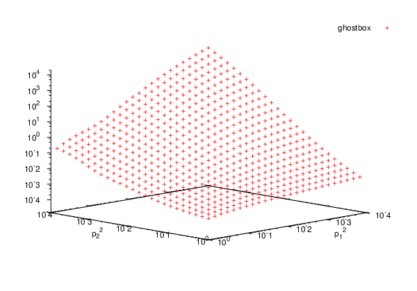
V The running coupling

The running coupling from the four-gluon vertex has already been given in eq.(3) and is repeated here for the convenience of the reader:

\displaystyle\alpha^{4g}(p^{2})

\displaystyle=

\displaystyle\frac{g^{2}}{4\pi}\,[\Gamma^{4g}(p^{2})]\,Z^{2}(p^{2})\,.

(63)

Here $\Gamma^{4g}(p^{2})$ denotes the dressing of the tree-level vertex structure $V_{1}$ and $Z(p^{2})$ denotes the dressing function of the gluon propagator. The value $\frac{g^{2}}{4\pi}=\alpha(\mu^{2})=0.97$ has also been given before. The resulting momentum dependence of the coupling is shown in Fig. 3 along with the running coupling from the ghost-gluon vertex. In the ultraviolet momentum region we observe that both couplings run like the usual inverse logarithm as well known from perturbation theory. Here we have universal behavior as dictated from gauge invariance. In the mid-momentum region we observe a steep rise of both couplings up to values of order $\alpha\sim 1$ . The coupling from the ghost-gluon vertex then keeps rising before freezing to an infrared fixed point, whereas the coupling from the four-gluon vertex decreases dramatically until it reaches a very small but nonzero fixed point in the deep infrared.

Before we discuss the implications of this behavior further, we wish to verify this numerical result from our analytical calculations in section III.3. There we found that

	${}^{IR}\Gamma_{gh}\left(p^{2}\right)$	$\displaystyle\approx$	$\displaystyle 1.045\cdot 10^{-4}\cdot\alpha(\mu^{2})\cdot N_{c}\cdot B^{4}\cdot(p^{2})^{-4\kappa}$		(64)
		$\displaystyle=$	$\displaystyle C_{gh}\cdot\alpha(\mu^{2})\cdot N_{c}\cdot B^{4}\cdot\left(p^{2}\right)^{-4\kappa}.$		(64)

In the infrared the gluon dressing function obeys the power-law

Z\left(p^{2}\right)=A\,\left(p^{2}\right)^{2\kappa}.

(65)

We then obtain

	$\displaystyle\alpha_{4g}\left(p^{2}\rightarrow 0\right)$	$\displaystyle=$	$\displaystyle\alpha\left(\mu^{2}\right)\cdot C_{gh}\cdot\alpha(\mu^{2})\cdot N_{c}\cdot B^{4}\cdot\left(p^{2}\right)^{-4\kappa}\cdot\left[A\left(p^{2}\right)^{2\kappa}\right]^{2}$		(66)
		$\displaystyle=$	$\displaystyle\left[\alpha\left(\mu^{2}\right)\cdot A\cdot B^{2}\right]^{2}\cdot N_{c}\cdot C_{gh},$		(66)

This expression is manifestly RG-invariant, since we know from the coupling of the ghost-gluon vertex that $\alpha(\mu^{2})AB^{2}$ is an RG-invariant. Also, since $\alpha(\mu^{2})=g^{2}/(4\pi)\sim 1/N_{c}$ and $A$ and $B$ are separately independent of $N_{c}$ [13, 22] as is $C_{gh}$ , the coupling is proportional to $1/N_{c}$ in agreement with the large $N_{c}$ counting rules.

Note that the combination $\alpha(\mu^{2})\,A\,B^{2}$ is equivalent to the running coupling from the ghost-gluon vertex at zero momentum [14]. Thus we can rewrite eq. (66) as

\displaystyle\alpha_{4g}\left(p^{2}\rightarrow 0\right)

\displaystyle=

\displaystyle[\alpha_{gh-gl}\left(p^{2}\rightarrow 0\right)]^{2}\cdot C_{gh}\cdot N_{c}

(67)

With $\alpha^{gh-gl}(0)\approx 8.92/N_{c}$ [14] and $C_{gh}=1.045\cdot 10^{-4}$ we then obtain

\displaystyle\alpha_{4g}\left(p^{2}\rightarrow 0\right)\approx\frac{0.0083}{N_{c}}.

(68)

This value agrees well with our numerical result.

In order to assess the implications of our findings it is worth noting that the corresponding coupling from the three-gluon vertex has a very similar behavior than the one of the four-gluon vertex shown in figure 3. In particular it also has an extremely small fixed point in the infrared, a maximum at intermediate momenta and a perturbative logarithmic tail in the ultraviolet [42]. We therefore find universality in the ultraviolet momentum region, as required from gauge invariance. In the infrared, all three couplings are qualitatively similar in the sense that they all go to an infrared fixed point (as already emphasized in [15]). However, there are huge qualitative differences between the coupling involving ghosts, $\alpha_{gh-gl}$ , and the other two couplings, $\alpha_{3g}$ and $\alpha_{4g}$ , that only involve gluonic correlators.

In this respect it is important to note, that the smallness of the infrared fixed point of the four-gluon vertex is rooted in the structure of the vertex-DSE. In section (III.3.1) we found, that the diagram involving ghosts is the one that gives the leading infrared behavior and determines the coefficient of the infrared power law $C_{gh}(p^{2})^{-4\kappa}$ of the four-gluon vertex. One reason why the coefficient $C_{gh}$ is small is a factor $1/216$ stemming from the projection on the tree-level tensor structure. The four propagators in the loop generate further suppression. Therefore the smallness of this coefficient can be attributed entirely to the structure of the DSE and does not depend on our choice for the ghost-gluon and three-gluon vertices.

Of course, the ghost box is only the first term in the skeleton expansion of the original ghost related diagram in the full DSE, eq. (12). It is known from ref. [15] that all terms in this expansion share the same infrared power law behavior and will therefore contribute to the coefficient $C_{gh}$ . Certainly, we cannot exclude that a summation of these terms will result in large changes compared to our value of $C_{gh}$ .

However, there is a systematic argument that indicates this may indeed be not the case. Consider once again the Dyson-Schwinger equation for the gluon propagator. In Fig. 4 we compare this equation with the corresponding flow equation in the functional renormalization group framework. From a systematic point of view, the DSE can be viewed as an integrated flow equation, so the physical content of the two equations is the same. However, there is an important structural difference between the two equations: In every diagram of the DSE we have one bare vertex, whereas in the flow equation, all vertices are dressed. As has been noted in [12] this leads to an interesting situation for small momenta: In the DSE the ghost-loop $(a)$ is the only diagram responsible for the leading contributions in the infrared, all other diagrams are suppressed by powers of momenta. In the flow equation, however, all diagrams share the same infrared exponent and therefore contribute to the coefficient of the resulting power law for the gluon dressing functions. Now, both equations are exact as they stand, so they should give the same results in the infrared. We also know that the ghost-gluon vertex is almost bare in the small momentum region. For this reasons we expect that the ghost-loop diagrams in the flow equations (first line) should be roughly similar in effect to the ghost-loop (a) in the gluon-DSE [43, 44]. Thus the infrared coefficients of all other diagrams in the flow equations have to either cancel, or should be much smaller than the coefficient of the ghost diagrams. Our result for the coupling from the four-gluon vertex together with the tentative result for the three-gluon vertex [42] indicates exactly this: since all these diagrams are roughly proportional to their corresponding coupling the gluonic diagrams in the flow equation are parametrically suppressed compared to the ghost-diagrams due to the smallness of the gluonic couplings in the infrared. This offers a natural explanation how the DSE and the renormalization group framework can agree in the infrared. In turn, this point suggests that the smallness of the four-gluon coupling may indeed be an effect which is robust beyond the leading order in the skeleton expansion.

In fact there is a further argument supporting this scenario. In [24] Zwanziger gave good arguments for an infrared effective theory dominated by the Faddeev-Popov determinant. He argued that all purely gluonic interactions switch off in the infrared and it is the geometry of the gauge group which then controls the infrared dynamics via the ghost content of the theory. This is exactly what we found here.

VI Summary

In this work we investigated the nonperturbative structure of the four-gluon vertex from (a truncated version of) its Dyson-Schwinger equation. We identified analytically the leading infrared and ultraviolet terms of this equation and found good agreement of this analysis with our numerical solution. We investigated the behavior of the three Bose symmetric tensor structures that can be constructed from a subset of the complete tensor basis of the vertex. The dressing functions of these three structures all show an infrared singular behavior with power laws in agreement with the results from naive power counting [15]. In the ultraviolet momentum region our solutions reproduce resummed perturbation theory.

The central result of our work concerns the running coupling from the four-gluon vertex, built from a combination of vertex dressing and the dressing function of the gluon propagator. Although in the ultraviolet momentum region the coupling agrees nicely with the one from the ghost-gluon vertex (as it should, according to gauge invariance), in the infrared we observe strong deviations. Whereas the coupling from the ghost-gluon vertex develops an infrared fixed point at around $\alpha_{gh-gl}(0)\approx 9/N_{c}$ , we find a much smaller fixed point at around $\alpha_{3g}(0)\approx 9\cdot 10^{-3}/N_{c}$ for the coupling from the four-gluon vertex.

Certainly, the stability of this finding has to be checked wrt further improvements of our truncation scheme. These have to include a study of the two-loop diagrams in the skeleton expansion of the ghost-part of the vertex DSE, since (only) these terms have the potential to change the infrared coefficients of the vertex and therefore the value of the infrared fixed point. However, on general grounds we are confident that the smallness of the running coupling from the four-gluon vertex is an important property which is stable wrt these improvements. As discussed in the last section, the reason is that this fact explains why the Dyson-Schwinger and the functional renormalization group equations for the two point functions of Yang-Mills theory agree in the infrared, although their structure is quite different. With small couplings from the three- and four-gluon vertices gluonic contributions to the infrared behaviour of the ghost and gluon FRGs are parametrically suppressed, leading to ghost dominance in agreement with the results from the DSEs. This finding also supports the notion of an infrared effective theory dominated from the Faddeev-Popov determinant proposed in [24].

Acknowledgments
We are grateful to Jan Pawlowski for discussions on the comparison between Dyson-Schwinger equations and the functional renormalization group equations. We also thank Reinhard Alkofer, Markus Huber and Kai Schwenzer for discussions and communicating preliminary results of ref. [42] to us. This work has been supported by the Helmholtz-University Young Investigator Grant VH-NG-332.

Appendix A The tensor basis

The tensor basis is constructed on the following building blocks of Lorentz- and color-tensors.
Color-tensors:

$C^{(1)}_{abcd}=\delta_{ab}\delta_{cd},$	$C^{(2)}_{abcd}=\delta_{ac}\delta_{bd},$	$C^{(3)}_{abcd}=\delta_{ad}\delta_{bc},$	$C^{(4)}_{abcd}=f_{abn}f_{cdn},$
$C^{(5)}_{abcd}=f_{acn}f_{dbn}$

Lorentz-tensors:

L^{\kappa\lambda\mu\nu}_{(1)}=\delta^{\kappa\lambda}\delta^{\mu\nu}

L^{\kappa\lambda\mu\nu}_{(2)}=\delta^{\kappa\mu}\delta^{\lambda\nu}

L^{\kappa\lambda\mu\nu}_{(3)}=\delta^{\kappa\nu}\delta^{\lambda\mu}

From these, a preliminary generator system of the tensor space can be constructed

$B_{1}=L^{(1)}C_{(1)}$	$B_{2}=L^{(1)}C_{(2)}$	$B_{3}=L^{(1)}C_{(3)}$	$B_{4}=L^{(1)}C_{(4)}$
$B_{5}=L^{(1)}C_{(5)}$	$B_{6}=L^{(2)}C_{(1)}$	$B_{7}=L^{(2)}C_{(2)}$	$B_{8}=L^{(2)}C_{(3)}$
$B_{9}=L^{(2)}C_{(4)}$	$B_{10}=L^{(2)}C_{(5)}$	$B_{11}=L^{(3)}C_{(1)}$	$B_{12}=L^{(3)}C_{(2)}$
$B_{13}=L^{(3)}C_{(3)}$	$B_{14}=L^{(3)}C_{(4)}$	$B_{15}=L^{(3)}C_{(5)},$

with the Lorentz/color-indices left implicit. The tree-level tensor-structure of the four-gluon vertex

$\displaystyle V^{(0)}$	$\displaystyle\propto$	$\displaystyle f_{abn}f_{cdn}(\delta^{\kappa\mu}\delta^{\lambda\nu}-\delta^{\kappa\nu}\delta^{\lambda\mu})$
		$\displaystyle+f_{acn}f_{bdn}(\delta^{\kappa\lambda}\delta^{\mu\nu}-\delta^{\kappa\nu}\delta^{\lambda\mu})$
		$\displaystyle+f_{adn}f_{bcn}(\delta^{\kappa\lambda}\delta^{\mu\nu}-\delta^{\kappa\mu}\delta^{\lambda\nu}),$

is not a member of the preliminary system. To construct a system containing the tree-level structure a Gram-Schmidt-algorithm is applied. It yields an orthogonal system of basis-tensors ${}^{(j)}T_{abcd}^{\kappa\lambda\mu\nu}$ . For projection purposes it is also useful to define normalised quantities ${(j)}U_{abcd}^{\kappa\lambda\mu\nu}$ such that

	$\displaystyle\left(c\cdot\,^{(j)}T_{abbcd}^{\kappa\lambda\mu\nu}\right)\cdot\,^{(k)}T_{abcd}^{\kappa\lambda\mu\nu}$	$\displaystyle\equiv$	${}^{(j)}U_{abcd}^{\kappa\lambda\mu\nu}\cdot\,^{(k)}T_{abcd}^{\kappa\lambda\mu\nu}$		(69)
		$\displaystyle=$	$\displaystyle\delta_{jk}.$		(69)

The basis system constructed this way is given by:

U_{(1)}=\frac{1}{108N_{c}^{2}(N_{c}^{2}-1)}\,(-B_{4}+2B_{5}+2B_{9}-B_{10}-B_{14}-B_{15})

U_{(2)}=\frac{1}{468N_{c}^{2}(N_{c}^{2}-1)}\,(-B_{4}+2B_{5}+2B_{9}-B_{10}+5B_{14}-B_{15})

U_{(3)}=\frac{1}{3510N_{c}^{2}(N_{c}^{2}-1)+\frac{123201}{4}(N_{c}^{2}-1)^{2}-21060N_{c}(N_{c}^{2}-1)}

\qquad\qquad\cdot(B_{4}-2B_{5}-2B_{9}+B_{10}+\frac{351}{8}B_{13}+\frac{29}{2}B_{14}+B_{15})

U_{(4)}=\frac{1}{\frac{276246}{25}N_{c}^{2}(N_{c}^{2}-1)+\frac{6472953}{100}(N_{c}^{2}-1)^{2}-\frac{1657476}{25}N_{c}(N_{c}^{2}-1)-\frac{848232}{25}(N_{c}^{2}-1)}

\qquad\qquad\cdot(B_{4}-2B_{5}-2B_{9}+B_{10}+\frac{306}{5}B_{12}-\frac{693}{40}B_{13}-\frac{263}{10}B_{14}+B_{15})

U_{(5)}=\frac{1}{5616N_{c}^{2}(N_{c}^{2}-1)+\frac{10138203}{25}(N_{c}^{2}-1)^{2}-33696N_{c}(N_{c}^{2}-1)-\frac{4363794}{25}(N_{c}^{2}-1)}

\qquad\qquad\cdot(-8B_{4}+16B_{5}+16B_{9}-8B_{10}+\frac{3141}{20}B_{11}-\frac{369}{20}B_{12}-\frac{369}{20}B_{13}+B_{14}-8B_{15})

U_{(6)}=\frac{1}{13816N_{c}^{2}(N_{c}^{2}-1)+294(N_{c}^{2}-1)^{2}-1372N_{c}(N_{c}^{2}-1)-294(N_{c}^{2}-1)}

\qquad\qquad\cdot(B_{4}-2B_{5}-2B_{9}+\frac{92}{3}B_{10}-\frac{7}{2}B_{11}+\frac{7}{4}B_{12}+\frac{7}{4}B_{13}-\frac{23}{6}B_{14}+B_{15})

U_{(7)}=\frac{1}{\frac{345536}{15}N_{c}^{2}(N_{c}^{2}-1)+96(N_{c}^{2}-1)^{2}-448N_{c}(N_{c}^{2}-1)-96(N_{c}^{2}-1)}

\qquad\qquad\cdot(\frac{136}{9}B_{4}-\frac{272}{9}B_{5}+\frac{2776}{90}B_{9}-\frac{104}{9}B_{10}-2B_{11}+B_{12}+B_{13}-\frac{1244}{90}B_{14}+\frac{136}{9}B_{15})

U_{(8)}=\frac{1}{\frac{1591288}{25}N_{c}^{2}(N_{c}^{2}-1)+\frac{10743516}{25}(N_{c}^{2}-1)^{2}-\frac{9486288}{25}N_{c}(N_{c}^{2}-1)-\frac{7776}{25}(N_{c}^{2}-1)}

\qquad\qquad\cdot(-B_{4}+2B_{5}+\frac{846}{5}B_{8}+\frac{193}{5}B_{9}+\frac{178}{5}B_{10}-\frac{18}{5}B_{11}+\frac{9}{5}B_{12}-\frac{81}{2}B_{13}-\frac{68}{5}B_{14}+B_{15})

U_{(9)}=\frac{1}{\frac{18614232}{125}N_{c}^{2}(N_{c}^{2}-1)+\frac{101940444}{125}(N_{c}^{2}-1)^{2}-\frac{111685392}{125}N_{c}(N_{c}^{2}-1)-\frac{48261744}{125}(N_{c}^{2}-1)}

\qquad\qquad\cdot(-B_{4}+2B_{5}+\frac{11304}{50}B_{7}-\frac{2844}{50}B_{8}-\frac{5606}{50}B_{9}+\frac{178}{5}B_{10}

\qquad\qquad\quad-\frac{18}{5}B_{11}-\frac{2736}{50}B_{12}+\frac{801}{50}B_{13}+\frac{1204}{50}B_{14}-B_{15})

U_{(10)}=\frac{1}{\frac{48940416}{625}N_{c}^{2}(N_{c}^{2}-1)+\frac{1828870727}{5625}(N_{c}^{2}-1)^{2}-\frac{46543936}{125}N_{c}(N_{c}^{2}-1)-\frac{48261744}{125}(N_{c}^{2}-1)}

\qquad\qquad\cdot(2B_{4}-4B_{5}+\frac{7074}{50}B_{6}-\frac{1386}{50}B_{7}-\frac{1386}{50}B_{8}+\frac{178}{50}B_{9}-\frac{356}{5}B_{10}

\qquad\qquad\quad-\frac{2817}{100}B_{11}+\frac{4}{3}B_{12}+\frac{4}{3}B_{13}-B_{14}+2B_{15})

U_{(11)}=\frac{1}{\frac{49098}{5}N_{c}^{2}(N_{c}^{2}-1)+1440(N_{c}^{2}-1)^{2}-6720N_{c}(N_{c}^{2}-1)-1440(N_{c}^{2}-1)}

\qquad\qquad\cdot(\frac{107}{6}B_{4}+\frac{25}{6}B_{5}+2B_{6}-B_{7}-B_{8}-\frac{37}{30}B_{9}-\frac{11}{2}B_{10}

\qquad\qquad\quad-8B_{11}+4B_{12}+4B_{13}-\frac{129}{10}B_{14}+\frac{107}{6}B_{15})

U_{(12)}=\frac{1}{5670N_{c}^{2}(N_{c}^{2}-1)+1440(N_{c}^{2}-1)^{2}-6720N_{c}(N_{c}^{2}-1)-1440(N_{c}^{2}-1)}

\qquad\qquad\cdot(\frac{25}{2}B_{4}-\frac{25}{6}B_{5}-2B_{6}+B_{7}+B_{8}-\frac{29}{6}B_{9}+\frac{11}{2}B_{10}

\qquad\qquad\quad+8B_{11}-4B_{12}-4B_{13}-\frac{41}{6}B_{14}-\frac{107}{6}B_{15})

U_{(13)}=\frac{1}{1080N_{c}^{2}(N_{c}^{2}-1)+7290(N_{c}^{2}-1)^{2}-6480N_{c}(N_{c}^{2}-1)}

\qquad\qquad\cdot(\frac{45}{2}B_{3}+5B_{4}+5B_{5}-\frac{9}{2}B_{8}-B_{9}-B_{10}-\frac{9}{2}B_{13}-B_{14}-B_{15})

U_{(14)}=\frac{1}{2520N_{c}^{2}(N_{c}^{2}-1)+13666(N_{c}^{2}-1)^{2}-14976N_{c}(N_{c}^{2}-1)-6048(N_{c}^{2}-1)}

\qquad\qquad\cdot(30B_{2}-\frac{14}{2}B_{3}-15B_{4}+5B_{5}-6B_{7}+\frac{3}{2}B_{8}+3B_{9}-B_{10}

\qquad\qquad\quad-6B_{12}+\frac{3}{2}B_{13}+3B_{14}-B_{15})

U_{(15)}=\frac{1}{1920N_{c}^{2}(N_{c}^{2}-1)+9720(N_{c}^{2}-1)^{2}-11520N_{c}(N_{c}^{2}-1)-6480(N_{c}^{2}-1)}

\qquad\qquad\cdot(25B_{1}-5B_{2}-5B_{3}+\frac{20}{3}B_{4}-\frac{40}{3}B_{5}-5B_{6}+B_{7}+B_{8}-\frac{4}{3}B_{9}+\frac{8}{3}B_{10}

\qquad\qquad\quad-5B_{11}+B_{12}+B_{13}-\frac{4}{3}B_{14}+\frac{8}{3}B_{15})

Appendix B The construction of the Bose symmetric tensor basis

To construct a basis of Bose-symmetric tensor-structures out of the structures given in appendix A, one first has to construct a matrix representation of the permutation group with respect to the tensor structures. A general tensor in the linear space ${\cal V}$ given by the tensor-basis from appendix A is represented by a vector

	$\displaystyle T$	$\displaystyle=$	$\displaystyle\sum_{i=1}^{15}a_{i}\cdot\,^{(i)}U_{\kappa\lambda\mu\nu}^{abcd}$		(70)
		$\displaystyle\equiv$	$\displaystyle(a_{1},a_{2},\dots,a_{15})$		(70)

An important feature of this tensor-basis, is that the tensor-structures constructed from it are closed under permutations of the external momenta. I.e. no tensor-structures not included from the very beginning are created by such permutations. This also means that permutations of the external momenta map the tensor space onto itself. Let $\cal P$ be a permutation of the external momenta, then

v\in{\cal V}\,:\quad{\cal P}v\in{\cal V}.

This means that there is a matrix-representation of the permutation. For the four-gluon vertex, there are $4!$ permutations. Let $M_{(j)}$ be the matrix-representation for the $j$ -th permutation. What one is interested in are the vectors $v\in{\cal V}$ that are invariant under all permutations. To find them one first has to find the eigenvectors with respect to the eigenvalue one for each member of the matrix-representation of the permutations. The eigenvalue one in general can have different geometrical multiplicities for each of these matrices. This restricts the dimension of the Bose symmetric tensor space. The maximum number of linear independent vectors in the Bose symmetric space is the difference of the lowest and the second lowest geometrical multiplicity of the eigenvalue one in the set of matrices of the representation of the permutations.

For the four-gluon vertex tensor-structures the lowest geometrical multiplicity of the eigenvalue one is five, while the second lowest is eight. Thus one ends up with an upper limit of three dimensions for the Bose symmetric tensor space. Having calculated the eigenvectors of the representation matrices, one can construct the full Bose symmetric linear tensor space. Let $e_{k,l}$ be the $l$ -th eigenvector with respect to eigenvalue one of the $k$ -permutation matrix.

M_{(j)}e_{k,l}=e_{k,l}.

Consider two permutations ${\cal P}_{1}$ and ${\cal P}_{2}$ , with matrix representations $M_{1}$ and $M_{2}$ . Denote the eigenvectors with respect to the eigenvalue one of these permutations as $v_{i}$ and $w_{i}$ respectively. Let the geometrical multiplicities of the eigenvalue one be $\mu_{1}$ and $\mu_{2}$ . The vectors, that are simultaneously included in the eigenspaces of two permutations, are found as the solution of the equation

\sum_{i=1}^{\mu_{1}}\xi_{i}\cdot v_{i}=\sum_{j=1}^{\mu_{2}}\bar{\xi}_{j}\cdot w_{j}.

(71)

If this coupled system of algebraic equations is determined it can easily be solved by standard methods. This is the case, when there is only one eigenvector that is invariant under all permutations. The case of an under-determined system also is not problematic. The overdetermined system (which occurs in the case of the four-gluon tensors) is more complicated. It is then useful to reformulate the problem. Let $A$ be the matrix, that is constructed from the column eigenvectors of both permutations in the following way

A=\Bigg(\Bigg(v_{1}^{T}\Bigg)\,\Bigg(v_{2}^{T}\Bigg)\,\dots\,\Bigg(v_{\mu_{1}}^{T}\Bigg)\,\Bigg(-w_{1}^{T}\Bigg)\,\Bigg(-w_{2}^{T}\Bigg)\,\dots\,\Bigg(-w_{\mu_{2}}^{T}\Bigg)\Bigg).

(72)

With this definition

A\cdot(\xi_{1},\dots,\xi_{\mu_{1}},\bar{\xi}_{1},\dots,\bar{\xi}_{\mu_{2}})^{T}=0

(73)

is equivalent to eq. (71). The non-trivial kernel of the matrix $A$ consists of $\mu_{1}+\mu_{2}$ -dimensional vectors, whose first $\mu_{1}$ components are the solution for the $\xi_{1}$ and the others are the solutions for the $\bar{\xi}_{j}$ . The kernel of the matrix can then be evaluated using standard methods. For the four-gluon vertex the result is given in the main body of this work, eq. (10).

Appendix C Decompositions of higher Green’s functions

In the following the decompositions of the reducible vertices in eq. (12) into one-particle irreducible vertices will be given [30, 29]. The reducible functions are denoted as $T$ and the irreducible as $\Gamma$ .

The decomposition of the four gluon reducible Green’s function:

\parbox{85.35826pt}{\begin{picture}{\put(0.0,0.0){\includegraphics[width=85.35826pt,keepaspectratio]{4GlueAmp1.eps}}\put(38.0,38.0){\hbox{\pagecolor{mygray}\scriptsize$T$}}}\end{picture}}=\parbox{85.35826pt}{\begin{picture}{\put(0.0,0.0){\includegraphics[width=85.35826pt,keepaspectratio]{4GlueAmp1.eps}}\put(38.0,38.0){\hbox{\pagecolor{mygray}\scriptsize$\Gamma$}}}\end{picture}}+\parbox{85.35826pt}{\begin{picture}{\put(0.0,0.0){\includegraphics[width=85.35826pt,keepaspectratio]{4GlueAmp2.eps}}\put(38.0,57.0){\hbox{\pagecolor{mygray}\scriptsize$\Gamma$}}\put(38.0,16.0){\hbox{\pagecolor{mygray}\scriptsize$\Gamma$}}}\end{picture}}+\parbox{85.35826pt}{\begin{picture}{\put(0.0,0.0){\includegraphics[width=85.35826pt,keepaspectratio]{4GlueAmp3.eps}}\put(39.0,57.0){\hbox{\pagecolor{mygray}\scriptsize$\Gamma$}}\put(39.0,16.0){\hbox{\pagecolor{mygray}\scriptsize$\Gamma$}}}\end{picture}}

(74)

The decomposition of the five gluon reducible function:

$\displaystyle=$	$\displaystyle\parbox{71.13188pt}{\begin{picture}{\put(0.0,0.0){\includegraphics[width=71.13188pt,keepaspectratio]{5GlueAmp1.eps}}\put(30.0,30.0){\hbox{\pagecolor{mygray}\scriptsize$\Gamma$}}}\end{picture}}+\parbox{85.35826pt}{\begin{picture}{\put(0.0,0.0){\includegraphics[width=85.35826pt,keepaspectratio]{5GlueAmp2.eps}}\put(38.0,57.0){\hbox{\pagecolor{mygray}\scriptsize$\Gamma$}}\put(38.0,16.0){\hbox{\pagecolor{mygray}\scriptsize$\Gamma$}}}\end{picture}}+\parbox{85.35826pt}{\begin{picture}{\put(0.0,0.0){\includegraphics[width=85.35826pt,keepaspectratio]{5GlueAmp3.eps}}\put(38.0,57.0){\hbox{\pagecolor{mygray}\scriptsize$\Gamma$}}\put(38.0,16.0){\hbox{\pagecolor{mygray}\scriptsize$\Gamma$}}}\end{picture}}$	(75)
	$\displaystyle\qquad\qquad+\parbox{85.35826pt}{\begin{picture}{\put(0.0,0.0){\includegraphics[width=85.35826pt,keepaspectratio]{5GlueAmp4.eps}}\put(38.0,57.0){\hbox{\pagecolor{mygray}\scriptsize$\Gamma$}}\put(38.0,16.0){\hbox{\pagecolor{mygray}\scriptsize$\Gamma$}}}\end{picture}}+\parbox{85.35826pt}{\begin{picture}{\put(0.0,0.0){\includegraphics[width=85.35826pt,keepaspectratio]{5GlueAmp5.eps}}\put(38.0,57.0){\hbox{\pagecolor{mygray}\scriptsize$\Gamma$}}\put(38.0,16.0){\hbox{\pagecolor{mygray}\scriptsize$T$}}}\end{picture}}$
	$\displaystyle\qquad\qquad+\parbox{85.35826pt}{\begin{picture}{\put(0.0,0.0){\includegraphics[width=85.35826pt,keepaspectratio]{5GlueAmp6.eps}}\put(38.0,57.0){\hbox{\pagecolor{mygray}\scriptsize$\Gamma$}}\put(38.0,16.0){\hbox{\pagecolor{mygray}\scriptsize$T$}}}\end{picture}}+\parbox{85.35826pt}{\begin{picture}{\put(0.0,0.0){\includegraphics[width=85.35826pt,keepaspectratio]{5GlueAmp7.eps}}\put(38.0,57.0){\hbox{\pagecolor{mygray}\scriptsize$\Gamma$}}\put(38.0,16.0){\hbox{\pagecolor{mygray}\scriptsize$T$}}}\end{picture}}$

Appendix D Analytical integration methods

D.1 Collected integrals

From ref.[45] we use:

(a)

	$\displaystyle\int_{0}^{\pi}\frac{\sin^{2\mu-1}x\,dx}{\left(1+2a\cos x+a^{2}\right)^{\nu}}$	$\displaystyle=$	$\displaystyle B\left(\mu,\frac{1}{2}\right)F\left(\nu,\nu-\mu+\frac{1}{2};\mu+\frac{1}{2};a^{2}\right)$
	$\displaystyle\left[\text{Re}\,\mu>0,\|a\|<1\right]\hskip 42.67912pt$

(76)

(b)

	$\displaystyle\int_{0}^{1}(1-x)^{\mu-1}x^{\nu-1}\,_{p}F_{q}(a_{1},\dots,a_{p};b_{1},\dots,b_{q};ax)dx=\hskip 142.26378pt$
	$\displaystyle=\frac{\Gamma(\mu)\Gamma(\nu)}{\Gamma(\mu+\nu)}\,_{p+1}F_{q+1}(\nu,a_{1},\dots,a_{p};\mu+\nu,b_{1},\dots,b_{q};a)\hskip 56.9055pt$

	$\displaystyle\left[\text{Re}\,\mu>0,\text{Re}\,\nu>0,p\leq q+1,\text{if}\,p=q+1,\text{then}\,\|a\|<1\right]\hskip 142.26378pt$

(77)

By partial integration, it can be seen:

$\displaystyle\int_{0}^{\pi}d\theta\cos\theta\times\frac{\sin^{2\mu-1}\theta}{\left(1+2a\cos\theta+a^{2}\right)^{\nu}}$	$\displaystyle=$	$\displaystyle-\frac{a\nu}{\mu}\int_{0}^{\pi}d\theta\frac{\sin^{2\mu+1}}{\left(1+2a\cos\theta+a^{2}\right)^{\nu+1}}$
	$\displaystyle=$	$\displaystyle-\frac{a\nu}{\mu}B\left(\mu+1,\frac{1}{2}\right)F\left(\nu+1,\nu-\mu+\frac{1}{2};\mu+\frac{3}{2};a^{2}\right)$
$\displaystyle\left[\text{Re}\,\mu>-1,\|a\|<1\right]\hskip 56.9055pt$

(78)

D.2 Integrating with the Chebyshev-expansion

A continuous function can be expanded in a series of polynomials. Most commonly one expands the function in a Taylor-series. But the convergence properties of a Taylor-series can fail to be sufficiently good, since the error of the approximation can be concentrated in a special region of the considered integration interval. When dealing with integrals on finite intervals, the Chebyshev-expansion can be an alternative. It has the advantage that the approximation error is smeared out over the interval. The integral of the original function is reduced to integrals over Chebyshev-polynomials.

The Chebyshev-polynomials are

T_{n}(x)=\cos(n\arccos(x)).

(79)

A function $f(x)$ can be expanded over these polynomials

f(x)\approx\sum_{j=1}^{N-1}c_{j}T_{j}(x)-\frac{c_{0}}{2},

(80)

with the coefficients

c_{j}=\frac{2}{N}\sum_{k=1}^{N}\cos\left(\frac{j(k-1/2)\pi}{N}\right)f\left[\cos\left(\frac{(k-1/2)\pi}{N}\right)\right],

(81)

where $N$ is the order of the expansion. The abscissas $\cos\left(\frac{(k-1/2)\pi}{N}\right)$ are the zeros of the n-th Chebyshev polynomial. For a more detailed discussion see [46].
To integrate a function using its Chebyshev-expansion, one transforms the variable, so that the integral is on the interval [-1,1].

	$\displaystyle\int_{a}^{b}dx\,f(x)$	$\displaystyle\stackrel{{\scriptstyle x=\tau(y)}}{{=}}$	$\displaystyle\frac{d\tau}{dy}\int_{-1}^{1}dy\sum_{j=0}^{N-1}c_{j}T_{j}(y)-\frac{c_{0}}{2}$		(82)
		$\displaystyle=$	$\displaystyle\frac{d\tau}{dy}\left(-c_{0}+\sum_{j=0}^{N-1}c_{j}\int_{-1}^{1}dy\,T_{j}(y)\right).$		(82)

Thus the integration has been reduced to an integration over Chebyshev-polynomials. The integral over the 0-th Chebyshev-polynomial yields $2$ , while the integral over the 1st vanishes.
The integral over the j-th Chebyshev polynomial yields

\int_{-1}^{1}dx\,T_{j}(x)=\frac{\cos(j\pi)+1}{1-j^{2}}.

(83)

Thus one obtains

\int_{a}^{b}dx\,f(x)\approx\frac{d\tau}{dy}\left(c_{0}+\sum_{j=2}^{N-1}c_{j}\frac{\cos(j\pi)+1}{1-j^{2}}\right).

(84)

Plugging in eq. (D.6) and denoting $y_{k}=\cos\left(\frac{(k-1/2)\pi}{N}\right)$ one finally gets

\displaystyle\int_{a}^{b}dx\,f(x)\approx\frac{2}{N}\frac{d\tau}{dy}\left(\sum_{k=1}^{N}f(y_{k})+\sum_{j=2}^{N-1}\sum_{k=1}^{N}\cos\left(\frac{j(k-1/2)\pi}{N}\right)f(y_{k})\frac{\cos(j\pi)+1}{1-j^{2}}\right).

(85)

D.3 The UV Integral

In the UV analysis of the Ghost- and the Gluon-Box integral of the form

I\equiv\int_{x}^{\infty}dy\frac{\left(\omega\log\left(\frac{y}{s}\right)+1\right)^{a}}{y^{n}}

(86)

occur. To evaluate them, one substitutes $z=\omega\log\left(\frac{y}{s}\right)+1$ yielding

I=\frac{e^{\frac{n-1}{\omega}}}{\omega s^{n-1}}\int_{z(x)}^{\infty}dz\,e^{-\frac{(n-1)z}{\omega}}z^{a}

(87)

and then $\xi=\frac{(n-1)z}{\omega}$ . One gets

	$\displaystyle I$	$\displaystyle=$	$\displaystyle\frac{e^{\frac{n-1}{\omega}}\omega^{a}}{s^{n-1}(n-1)^{a+1}}\int_{\xi(z(x))}^{\infty}d\xi\,e^{-\xi}\xi^{a}$		(88)
		$\displaystyle=$	$\displaystyle\frac{e^{\frac{n-1}{\omega}}\omega^{a}}{s^{n-1}(n-1)^{a+1}}\Gamma\left(a+1,(n-1)\left(\log\left(\frac{x}{s}\right)+\frac{1}{\omega}\right)\right).$		(88)

Since $x$ is large in the region of interest, one can employ the asymptotic expansion

\Gamma(a,x)=x^{a-1}\,e^{-x}\left[\sum_{m=0}^{M-1}\frac{(1-a)_{m}}{(-x)^{m}}+O(|x|^{-M})\right],

(89)

with the Pochhammer-symbol $(a)_{m}$

(a)_{0}=1,\quad(a)_{n}=\frac{\Gamma(a+n)}{\Gamma(a)}=a(a+1)\ldots(a+n-1).

(90)

Keeping only the first order of the series, one results in

\int_{x}^{\infty}dy\,\frac{\left(\omega\log\ \left(\frac{y}{s}\right)+1\right)^{a}}{y^{n}}\approx\frac{\left(\omega\log\left(\frac{x}{s}\right)+1\right)^{a}}{(n-1)x^{n-1}}.

(91)

References

[1] G. M. Prosperi, M. Raciti and C. Simolo, Prog. Part. Nucl. Phys. 58 (2007) 387 [arXiv:hep-ph/0607209].
[2] P. Boucaud, J. P. Leroy, J. Micheli, O. Pene and C. Roiesnel, JHEP 9810 (1998) 017 [arXiv:hep-ph/9810322].
[3] M. Della Morte, R. Frezzotti, J. Heitger, J. Rolf, R. Sommer and U. Wolff [ALPHA Collaboration], Nucl. Phys. B 713 (2005) 378 [arXiv:hep-lat/0411025].
[4] O. Kaczmarek and F. Zantow, Phys. Rev. D 71 (2005) 114510 [arXiv:hep-lat/0503017].
[5] A. Cucchieri and T. Mendes, Braz. J. Phys. 37 (2007) 484 [arXiv:hep-ph/0605224].
[6] E. M. Ilgenfritz, M. Muller-Preussker, A. Sternbeck and A. Schiller, arXiv:hep-lat/0601027. A. Sternbeck, K. Maltman, L. von Smekal, A. G. Williams, E. M. Ilgenfritz and M. Muller-Preussker, arXiv:0710.2965 [hep-lat].
[7] C. Allton, A. Trivini, M. Teper and A. Trivini, arXiv:0710.1138 [hep-lat].
[8] D. V. Shirkov and I. L. Solovtsov, Phys. Rev. Lett. 79 (1997) 1209 [arXiv:hep-ph/9704333].
[9] D. V. Shirkov and I. L. Solovtsov, Theor. Math. Phys. 150 (2007) 132 [arXiv:hep-ph/0611229].
[10] H. Gies, Phys. Rev. D 66, 025006 (2002) [arXiv:hep-th/0202207].
[11] J. Braun and H. Gies, Phys. Lett. B 645 (2007) 53 [arXiv:hep-ph/0512085].
[12] C. S. Fischer and J. M. Pawlowski, Phys. Rev. D 75, 025012 (2007) [arXiv:hep-th/0609009].
[13] L. von Smekal, R. Alkofer and A. Hauck, Phys. Rev. Lett. 79 (1997) 3591 [arXiv:hep-ph/9705242].
[14] C. Lerche and L. von Smekal, Phys. Rev. D 65, 125006 (2002) [arXiv:hep-ph/0202194].
[15] R. Alkofer, C. S. Fischer and F. J. Llanes-Estrada, Phys. Lett. B 611, 279 (2005) [arXiv:hep-th/0412330]. arXiv:hep-ph/0607293.
[16] S. J. Brodsky, S. Menke, C. Merino and J. Rathsman, Phys. Rev. D 67, 055008 (2003) [arXiv:hep-ph/0212078].
[17] M. Baldicchi, A. V. Nesterenko, G. M. Prosperi, D. V. Shirkov and C. Simolo, arXiv:0705.1695 [hep-ph].
[18] R. Alkofer and L. von Smekal, Phys. Rept. 353, 281 (2001) [arXiv:hep-ph/0007355].
[19] J. M. Pawlowski, Annals Phys. 322 (2007) 2831 [arXiv:hep-th/0512261].
[20] C. S. Fischer, J. Phys. G 32 (2006) R253 [arXiv:hep-ph/0605173].
[21] W. Celmaster and R. J. Gonsalves, Phys. Rev. D 20 (1979) 1420.
[22] C. S. Fischer and R. Alkofer, Phys. Lett. B 536 (2002) 177 [arXiv:hep-ph/0202202].
[23] D. Zwanziger, Phys. Rev. D 65, 094039 (2002) [arXiv:hep-th/0109224].
[24] D. Zwanziger, Phys. Rev. D 67 (2003) 105001 [arXiv:hep-th/0206053]; Phys. Rev. D 69 (2004) 016002 [arXiv:hep-ph/0303028].
[25] M. Baker and C. k. Lee, Phys. Rev. D 15 (1977) 2201 [Erratum-ibid. D 17 (1978) 2182].
[26] F. T. Brandt and J. Frenkel, Phys. Rev. D 33 (1986) 464.
[27] J. Papavassiliou, Phys. Rev. D 47, 4728 (1993).
[28] M. Stingl, Z. Phys. A 353, 423 (1996) [arXiv:hep-th/9502157].
[29] L. Driesen, J. Fromm, J. Kuhrs and M. Stingl, Eur. Phys. J. A 4, 381 (1999) [arXiv:hep-th/9808152].
[30] L. Driesen and M. Stingl, Eur. Phys. J. A 4, 401 (1999) [arXiv:hep-th/9808155].
[31] J. A. M. Vermaseren, arXiv:math-ph/0010025.
[32] F. D. R. Bonnet, P. O. Bowman, D. B. Leinweber, A. G. Williams and J. M. Zanotti, Phys. Rev. D 64 (2001) 034501 [arXiv:hep-lat/0101013].
[33] A. Sternbeck, E. M. Ilgenfritz, M. Mueller-Preussker and A. Schiller, Phys. Rev. D 72 (2005) 014507 [arXiv:hep-lat/0506007].
[34] J. C. Taylor, Nucl. Phys. B 33 (1971) 436.
[35] W. Schleifenbaum, A. Maas, J. Wambach and R. Alkofer, Phys. Rev. D 72, 014017 (2005) [arXiv:hep-ph/0411052].
[36] A. Sternbeck, E. M. Ilgenfritz, M. Muller-Preussker, A. Schiller and I. L. Bogolubsky, PoS LAT2006, 076 (2006) [arXiv:hep-lat/0610053].
[37] A. Cucchieri, A. Maas and T. Mendes, Phys. Rev. D 74, 014503 (2006) [arXiv:hep-lat/0605011]; arXiv:0803.1798 [hep-lat].
[38] P. Watson and R. Alkofer, Phys. Rev. Lett. 86 (2001) 5239 [arXiv:hep-ph/0102332].
[39] N. Nakanishi and I. Ojima, World Sci. Lect. Notes Phys. 27, 1 (1990).
[40] A. Cucchieri and T. Mendes, arXiv:0710.0412 [hep-lat].
[41] A. Sternbeck, L. von Smekal, D. B. Leinweber and A. G. Williams, arXiv:0710.1982 [hep-lat].
[42] R. Alkofer, M. Huber and K. Schwenzer, in preparation.
[43] J. M. Pawlowski, D. F. Litim, S. Nedelko and L. von Smekal, Phys. Rev. Lett. 93 (2004) 152002 [arXiv:hep-th/0312324].
[44] C. S. Fischer and H. Gies, JHEP 0410, 048 (2004) [arXiv:hep-ph/0408089].
[45] I.Gradshteyn and I.W. Ryzhik, Tables of Integrals, Series and Products. Academic Press, New York, 1965.,
[46] J. C. R. Bloch, arXiv:hep-ph/0208074.