On the Evolution of Differentiated Multicellularity

Martin Willensdorfer

Program for Evolutionary Dynamics
Department of Molecular and Cellular Biology
Harvard University, Cambridge, MA 02138, USA.
E-mail: willensd@fas.harvard.edu

Keywords: differentiation, soma, specialized cells, reproductive cells, fitness,
Running Title: Evolution of Multicellularity

Abstract

Most conspicuous organisms are multicellular and most multicellular organisms develop somatic cells to perform specific, non-reproductive tasks. The ubiquity of this division of labor suggests that it is highly advantageous. In this paper, I present a model to study the evolution of specialized cells. The model allows for unicellular and multicellular organisms that may contain somatic (terminally differentiated) cells. Cells contribute additively to a quantitative trait. The fitness of the organism depends on this quantitative trait (via a benefit function), the size of the organism, and the number of somatic cells. This model allows one to determine when somatic cells are advantageous and to calculate the optimum number (or fraction) of reproductive cells. I show that the fraction of reproductive cells is always surprisingly high. If somatic cells are very small, they can outnumber reproductive cells but their biomass is still less than the biomass of reproductive cells. Only for non-concave benefit functions can the biomass of somatic cell exceed the biomass of reproductive cells. I discuss the biology of primitive multicellular organisms with respect to the model predictions. I find good agreement and outline how this work can be used to guide further quantitative studies of multicellularity.

1 Introduction

Every organism is exposed to mutations that cause variation in inherited traits. Competition between slightly different organisms leads to the proliferation of variants that increase fitness. Most adaptations will fine-tune existing systems but some adaptations lead to new features. The evolution of multicellularity was clearly such an adaptation. It opened a door to a whole new world of possibilities (Bonner, 1965; Buss, 1988; Maynard-Smith & Szathmary, 1997; Bonner, 2001; Knoll, 2003; Nowak, 2006).

In their simplest form multicellular organisms are just clusters of identical cells. Such undifferentiated multicellular organisms can evolve fairly quickly through mutations of surface proteins (Boraas et al., 1998; Rainey & Travisano, 1998; Velicer & Yu, 2003). Cells in such clonal aggregates do not have to compete against each other for reproduction since they are genetically identical (Buss, 1988). This alleviation of reproductive competition has a profound effect. It allows for a division of labor. Cells can specialize on non-reproductive (somatic) tasks and peacefully die since their genes are passed on by genetically identical reproductive cells which benefited from the somatic function. This division of labor turns multicellular organisms into more than just lumps of cells. They contain cells that are different in function and appearance. Today a plethora of differentiated organisms exist, demonstrating the evolutionary success of division of labor.

Most theoretical studies of multicellularity analyze the change in level of selection and the consequences for reproductive competition (Buss, 1988; Maynard-Smith & Szathmary, 1997; Michod, 1997; Michod & Roze, 1997; Michod & Roze, 2001). In this paper I study which conditions make differentiated multicellularity desirable. When does a differentiated multicellular organism have higher fitness than an undifferentiated or unicellular organism? In the model presented here, an organism’s fitness depends on a quantitative trait. The quantitative trait is determined by the number and types of cells in the multicellular organism. The mathematical model allows one to study which kind of benefits multicellularity must convey to compensate for its disadvantages. I calculate how much (compared to a reproductive cell) a somatic cell has to contribute to the quantitative trait to make division of labor advantageous and determine the optimum number/fraction of somatic cells.

The following section describes the model in detail. In the Results, I will first consider the evolution of undifferentiated multicellularity. To study the evolution of differentiated multicellularity I analyze the fitness of organisms of constant size. Thereafter, I study multicellularity in organisms where the size of the organism and the fraction of somatic cells is governed by the same evolutionary forces. In the Discussion, I use the insights from my analysis to discuss a broad spectrum of primitive multicellular organisms.

2 The model

In this work I use the rate of biomass production as a measure of fitness. The rate of biomass production captures an organism’s ability to grow and reproduce. It denotes how much new biomass per unit of existing biomass an organism can generate per unit of time. For organisms of equal size, production rates are equivalent to fitness (number of new organisms produced per organism per unit of time). The model considers how somatic cells, body size, and benefits of multicellularity affect the rate of production. I distinguish between reproductive and somatic cells but allow for only one kind of somatic cell. Somatic cells are different from reproductive cells in that they are terminally differentiated. Their biomass does not contribute to the next generation. Reproductive cells, on the other hand, contribute to the next generation. They can be asexually or sexually reproductive.

To derive how somatic cells affect fitness, let us first assume that multicellularity and organism size have no effect on the rate of production. In this case, as illustrated in Figure 2, a unicellular organism has the same fitness as a four-cell organism because four unicellular organisms produce 16 unicellular descendants (16 cells) after two cell divisions, and one four-cell organism produces four four-cell descendants (16 cells). Indeed, if size and multicellularity have no effect on fitness, then all organisms that are entirely composed of reproductive cells will have the same fitness. Let us use a four-cell organism to derive the cost of somatic cells.

Figure 2: Cost of somatic cells in differentiated organisms. If the rate of production is independent of organism size, then every undifferentiated organism has the same fitness. Four unicellular organisms produce 16 cells after two cell division (first row), as does one four-cell organism (second row). A four-cell organism with two somatic cells (third row) produces half the biomass of an undifferentiated organism, because only half its cells are able to contribute to the next generation. If the two somatic cells are extremely small (fourth row) then nearly all the biomass is concentrated in reproductive cells and fitness is equal to the fitness of an undifferentiated organism. In general the fitness of a differentiated organism relative to an undifferentiated is given by the fraction of biomass that is used for reproduction, that is, by

N_{r}/(N_{r}+BN_{s})=1-BN_{s}/(N_{r}+BN_{s})

, where

B

is the size of a somatic cell relative to the size of a reproductive cell.

The cost of somatic cells stems from their inability to contribute directly to the next generation. To quantify this cost, we can compare the rate of production of a four-cell organism that has two somatic cells with the rate of production of a four-cell organism without somatic cells. As shown in Figure 2, the effect of somatic cells depends on their size. If the somatic cells are negligibly small, then the rate of production of a differentiated organism is equal to the rate of production of an undifferentiated organism (forth row in Fig. 2). If somatic cells are as large as reproductive cells, then a differentiated four-cell organism with two somatic cells is able to produce only two new four-cell organisms (8 cells) whereas the undifferentiated organism produces four new organisms (16 cells). Hence the rate of production of the differentiated organism is $1/2$ the rate of production of the undifferentiated organism. In general, the rate of production (fitness) is reduced by the fraction of biomass that does not contribute to the next generation.

In the following we will assign parameters so the biomass and number of somatic and reproductive cells to quantify this fitness reduction. I use the Greek letters $\alpha$ and $\beta$ to denote the biomass of a reproductive and a somatic cell, respectively, in the adult organism, As we will see, it is sufficient to consider the size of a somatic cell relative to the size of a reproductive cell. Let $B=\beta/\alpha$ denote this size ratio. Let $N_{r}$ and $N_{s}$ denote the number of reproductive and somatic cells. An adult organism is composed of $N=N_{r}+N_{s}$ cells and has a body mass of $\alpha N_{r}+\beta N_{s}$ . Of that biomass $\beta N_{s}$ rests in somatic (sterile) cells and $\alpha N_{r}$ in reproductive cells. Hence, $\beta N_{s}/(\alpha N_{r}+\beta N_{s})$ of the organism’s biomass is lost in each generation and constitutes the cost of somatic cells. The fitness of an organism with somatic cells relative to the fitness of an organism without somatic cells is given by

1-\beta N_{s}/(\alpha N_{r}+\beta N_{s})=\alpha N_{r}/(\alpha N_{r}+\beta N_{s})=N_{r}/(N_{r}+BN_{s}),

(1)

for $B=\beta/\alpha$ as defined above.

So far I have assumed that the rate of production is independent of the organism size and that multicellularity does not convey benefits. An overwhelming amount of empirical data shows that the rate of production decreases with the body mass of an organism (Peters, 1986). In particular the annual rate of production per average biomass scales with $W^{-\gamma}$ , where $W$ denotes the average body mass of an adult organism and $\gamma$ is a scaling factor. This relationship holds from unicellular organisms to mammals, with body masses ranging from approximately $10^{-10}$ to $10^{3}$ kg. As summarized by Peters (1986, p. 134), the exponent $\gamma$ might range from $0.23$ to $0.37$ . For small organisms $\gamma$ is close to $1/4$ , the typical allometric exponent of size. I will therefore use $\gamma=1/4$ to discuss quantitative results. From above, we know that the adult body mass of an organism in this model is given by $W=\alpha N_{r}+\beta N_{s}$ . Hence, the rate of production decreases by the factor $(\alpha N_{r}+\beta N_{s})^{-\gamma}$ .

I model the advantages of multicellularity as a function of the number of reproductive and somatic cells. Let $f(N_{r},N_{s})$ denote this benefit function. Therefore, the fitness of a multicellular organism is given by

$\displaystyle F(N_{r},N_{s})$	$\displaystyle=$	$\displaystyle\textnormal{cost of somatic cells}\times\textnormal{cost of size}\times\textnormal{benefit of multicellularity}$	(2)
	$\displaystyle=$	$\displaystyle\frac{\alpha N_{r}}{\alpha N_{r}+\beta N_{s}}\times(\alpha N_{r}+\beta N_{s})^{-\gamma}\times f(N_{r},N_{s})$
	$\displaystyle=$	$\displaystyle\frac{\alpha N_{r}}{(\alpha N_{r}+\beta N_{s})^{1+\gamma}}f(N_{r},N_{s})$
	$\displaystyle\propto$	$\displaystyle\frac{N_{r}}{(N_{r}+BN_{s})^{1+\gamma}}f(N_{r},N_{s}),$

where $B=\beta/\alpha$ is the size of a somatic cell relative to the size of a reproductive cell.

This model confirms common sense. If multicellularity does not affect fitness, that is, $f(N_{r},N_{s})=\textnormal{constant}$ , then a unicellular organism has a higher fitness than a multicellular organism since $F(N_{r},N_{s})<F(N_{r},0)<F(1,0)$ for $N_{r}>1$ and $N_{s}>0$ . For undifferentiated multicellularity the fitness of an organism is given by $N_{r}^{-\gamma}f(N_{r},0)$ and multicellularity is only advantageous if it conveys benefits that compensate for the disadvantages caused by the size increase. In other words, $f(N_{r},0)$ has to increase more steeply than $N_{r}^{-\gamma}$ decreases.

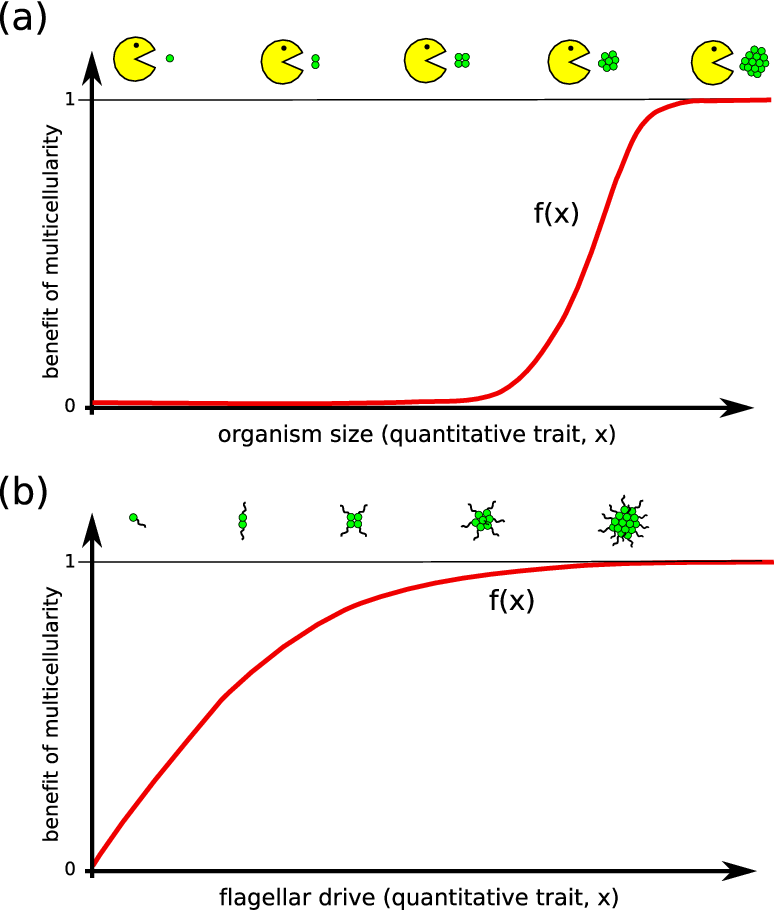
Central to my analysis of multicellularity is the function $f(N_{r},N_{s})$ , which captures the benefit of multicellularity. I will assume that somatic and reproductive cells contribute to a quantitative trait, $x$ , and that the benefit of multicellularity is a function, $f(x)$ , of this trait. For simplicity, I illustrate this approach by formulating predator evasion and flagellation in terms of this model.

For predator evasion, the quantitative trait is given by the size of the organism. It increases with the number of cells. Its value determines to which extent the organism is able to evade predation. If the organism is big enough, the predator is unable to ingest it and the benefit of multicellularity, $f(x)$ , is close to $1$ . For small organisms predation might be severe and $f(x)$ close to $0$ . One can expect a steep increase of $f(x)$ as the organism size surpasses the maximum particle size the predator can ingest. Figure 4a shows a benefit function that could be used to describe predator evasion.

For flagellation, the quantitative trait is given by the flagellar drive that the cells of the organism provide. The more cells, the more flagellar drive, which improves the organism’s ability to maintain its position in a favorable environment. For this example the benefit function can be expected to be concave. An initial increase in flagellar drive might be very beneficial by allowing the organism to maintain its position. At some point, however, the organism has enough flagellar drive to maintain its position for most of the time and a further increase in flagellar drive does not yield a substantial benefit. Figure 4b shows a benefit function that could be used to model benefits from flagellation.

Figure 4: The use of benefit functions to model the benefit of multicellularity. (a) Predator evasion: Multicellularity can be beneficial by allowing the multicellular organism to evade predation. We can model this benefit as a function of the organism size (a quantitative trait). Multicellularity is not beneficial if the size of the organism does not exceed the predators upper prey size limit. Large benefits can be expected for size increases that surpasses this prey size limit. Once this threshold is exceeded and the organism immune against predation, further size increases bring little additional benefits. (b) Flagellation: Multicellularity can also increase the motility of an organism by increasing its flagellar drive (a quantitative trait). Initial increases in motility can bring large benefits because they increase an organism’s ability to reach favorable environments. At some point, however, a further increase in flagellar drive brings little benefits because the organism is already able to access the most favorable environment.

As we will see, my analysis of this model does not require an exact specification of the benefit function. But it is necessary to make assumptions about the contribution of individual cells to the quantitative trait.

I am mainly interested in the evolution of early multicellular organisms composed of few cells for which it is reasonable to assume (at least as an approximation) that cells contribute additively to the quantitative trait. I use the letters $a$ and $b$ to denote the contribution of a reproductive and a somatic cell to the quantitative trait. In an organism with $N_{r}$ reproductive and $N_{s}$ somatic cells, the quantitative trait, $x$ , is given by

x=aN_{r}+bN_{s}.

(3)

Hence, we have

f(N_{r},N_{s})=f(aN_{r}+bN_{s}).

(4)

Let $A=a/b$ denote the contribution of a reproductive cell relative to the contribution of a somatic cell. Since somatic cells are specialized cells and free of reproductive constraints, they will generally contribute more to the trait than reproductive cells ( $b>a$ ), hence, $A=a/b\in[0,1]$ . Furthermore, I consider organisms where somatic cells are usually smaller than reproductive cells ( $\beta\leq\alpha$ ) and, hence, $B=\beta/\alpha\in(0,1]$ .

To simplify the analysis, I scale the argument for $f$ so that $b=1$ , that is, a somatic cell contributes one unit to the quantitative trait. By using $A=a/b$ and rescaling the argument for $f$ , we can rewrite (2) as

\displaystyle F

\displaystyle\propto

\displaystyle\frac{N_{r}}{(N_{r}+BN_{s})^{1+\gamma}}f\left(AN_{r}+N_{s}\right).

(5)

Note that if the contribution of reproductive cells to the quantitative trait is insignificant (i.e., $AN_{r}+N_{s}\approx N_{s}$ ) then the benefit of multicellularity is simply a function of the number of somatic cells.

So far I have not made any assumptions about $f(x)$ . To simplify the analysis I restrict $f(x)$ to monotone increasing and bound functions. Both constraints are reasonable. An increase of the quantitative trait should not lead to a decrease in fitness, and the fitness of an organism cannot be increased infinitely. As mentioned earlier, $f(x)$ is scaled such that $\lim\limits_{x\rightarrow\infty}f(x)=1$ .

Symbol	Interpretation
$N_{r}$	Number of reproductive cells
$N_{s}$	Number of somatic cells (an organism is undifferentiated if $N_{s}=0$ )
$\alpha$	Size of a reproductive cell
$\beta$	Size of a somatic cell
$B=\beta/\alpha$	The size of a somatic cell relative to the size of a reproductive cell; $B$ is bound to $[0,1]$
$a$	Contribution of a reproductive cell to the quantitative trait
$b$	Contribution of a somatic cell to the quantitative trait
$A=a/b$	Contribution of a reproductive cell to the quantitative trait relative to the contribution of a somatic cell; $A$ is bound to $[0,1]$
$x$	The value of the quantitative trait
$f(x)$	The benefit function. It captures the extend to which the organism benefits from the quantitative trait. The benefit function is scaled such that $\lim_{x\rightarrow\infty}f(x)=1$ .
$\gamma$	The allometric exponent which is approximately $1/4$

Table 1: Notation summary

Table 1 summarizes the variables and parameters used in this model.

3 Results

I am interested in the kind of benefit functions, $f(x)$ , that promote the evolution of multicellularity. I am also interested in how much a somatic cell has to contribute to the quantitative trait (relative to reproductive cells) to compensate for the loss in somatic biomass. I calculate the optimum fraction of reproductive cells and the optimum fraction of reproductive biomass. This allows us to determine under which conditions undifferentiated or differentiated multicellularity evolves and to infer on the composition of early differentiated multicellular organisms.

First, I analyze conditions for the evolution of undifferentiated multicellularity. Thereafter I study the evolution of somatic cells in organisms of constant size. I study the unconstrained model last. In the unconstrained model the size of the organism and the fraction of somatic cells is governed by the benefit function $f(x)$ . I show that it is possible to calculate the optimum fraction of reproductive cells and that this fraction is independent of the benefit function $f(x)$ .

3.1 Undifferentiated multicellularity

The evolution of undifferentiated multicellularity corresponds to an evolutionary transition from organisms composed of one (reproductive) cell to organisms composed of several identical (also reproductive) cells. Undifferentiated multicellular organisms have, per definition, no somatic cells ( $N_{s}=0$ ). For $N_{s}=0$ , the fitness (2) simplifies to

F(N_{r})\propto N_{r}^{-\gamma}f(N_{r},0).

(6)

Multicellularity ( $N_{r}>1$ ) is only advantageous if $N_{r}^{-\gamma}f(N_{r},0)>f(1,0)$ . In other words, the benefit function $f(N_{r},0)$ has to increase faster than $N_{r}^{-\gamma}$ decreases.

I employ this simple case to illustrate the method that will be used to analyze the more complex cases. I would like to know for which functions $f(x)$ multicellularity is advantageous and what the optimum number of reproductive cells is. To get a general idea of how $f(x)$ affects fitness, we can determine the functions $f(x)$ for which the fitness is constant with respect to $N_{r}$ . Let $f_{\textnormal{iso}}(x)$ denote these functions. I refer to them as isolines since they join points of equal fitness. They are analogous to the lines on topographic maps that join points of equal altitude. These isolines can be used to illustrate the fitness landscape with respect to benefit functions $f(x)$ . The fitness of an undifferentiated organism is given by $F=N_{r}^{-\gamma}f(aN_{r})$ and constant if $f(aN_{r})\propto N_{r}^{\gamma}$ . Substituting $x=aN_{r}$ , we get

f_{\textnormal{iso}}(x)\propto x^{\gamma}.

(7)

The gray curves in Figure 5 show these isolines. With the knowledge of these isolines it is easy to determine which functions, $f(x)$ , promote the evolution of multicellularity. It is also simple to determine the optimum number of reproductive cells. An organism with $N_{r}$ reproductive cells has $x=aN_{r}$ as value for the quantitative trait. We have an optimum $x_{\textnormal{opt}}=aN_{r,\textnormal{opt}}$ if $f(x)\leq f_{\textnormal{iso}}(x)$ for the isoline with $f(x_{\textnormal{opt}})=f_{\textnormal{iso}}(x_{\textnormal{opt}})$ . In a continuous setting the optimum satisfies $\frac{\partial}{\partial x}f(x_{\textnormal{opt}})=\frac{\partial}{\partial x}f_{\textnormal{iso}}(x_{\textnormal{opt}})$ for the isoline with $f(x_{\textnormal{opt}})=f_{\textnormal{iso}}(x_{\textnormal{opt}})$ .

To interpret isoline plots, it might be useful to keep the analogy with topographic maps in mind. One can think of $x$ as the distance traveled along a particular trail, $f(x)$ , in a mountainous region. The highest point, in our case the optimum, $x_{\textnormal{opt}}$ , is reached if the trail “brushes” the highest contour line along the trail, $f(x_{\textnormal{opt}})=f_{\textnormal{iso}}(x_{\textnormal{opt}})$ . None of the points along the trail will be above this contour line, $f(x)\leq f_{\textnormal{iso}}(x)$ .

Figure 5 shows two linear and one concave benefit function. The black bullets indicate the optimum for each benefit function. As one can see, a linear benefit function will always promote the evolution of multicellularity and will increase $f(x)$ until it reaches a value close to one. A concave benefit function reaches the optimum earlier and results in smaller organisms. Undifferentiated multicellularity would not evolve if $f(x)$ increases slower than the isolines. In particular, multicellularity would not evolve if $f(a)>2^{-\gamma}$ . For $\gamma=1/4$ , we have $2^{-\gamma}=0.84$ and multicellularity would not evolve if unicellular organisms are able to benefit from the quantitative trait more than 84% of its full potential.

3.2 Differentiated multicellularity in organisms of constant size

In the previous section I have shown that undifferentiated multicellularity is advantageous for many benefit functions. In the following I will analyze the evolution of somatic cells (differentiated multicellularity). For simplicity, I will first analyze the evolution of somatic cells in organisms of constant size.

From a biological perspective it is relevant to consider organisms of constant size, since many benefits of undifferentiated multicellularity imply constraints on the size of the organism. Predator evasion, for example, is known to promote the evolution of undifferentiated multicellularity (Boraas et al., 1998). An organism that uses multicellularity to evade predation is obviously constrained with respect to size. It has to be larger than the largest particle that the predator can feed on. Replacing nine large reproductive cells with nine small somatic cells could decrease its size to dangerous levels.

For simplicity, I will first assume that somatic and reproductive cells have the same size ( $B=1$ ) and explore the more general case of $B<1$ thereafter.

3.2.1 Somatic cells are as large as reproductive cells ( $B=1$ )

The size of an organism is given by $S=\alpha N_{r}+\beta N_{s}$ . If somatic and reproductive cells have the same size ( $B=\beta/\alpha=1$ ), then the size of the organism can only be held constant if the number of cells that compose this organism is constant, that is, $N=N_{r}+N_{s}=\textnormal{constant}$ . In this case the fitness, $F(N_{r},N_{s})$ , depends on one variable instead of two. Using $N_{r}$ as this variable we can rewrite (2) as

F\propto N_{r}f\left[N-(1-A)N_{r}\right],

(8)

because the trait value of an organism with $N$ cells is given by $x=N-(1-A)N_{r}$ . Hence, the quantitative trait of an organism of size $N$ has a value of at least $AN$ (if $N_{r}=N$ ) and at most $N-1+A$ (if $N_{r}=1$ ). The fitness of an organism is constant if $f\left[N-(1-A)N_{r}\right]\propto N_{r}^{-1}$ . Expressing the number of reproductive cells, $N_{r}$ , in terms of the quantitative trait, $x$ , we get

f_{\textnormal{iso}}(x)\propto(N-x)^{-1}.

(9)

Since we rescaled $f(x)$ so that a somatic cell contributes one unit to the quantitative trait, we can interpret $N$ in (9) as the value of the quantitative trait of an organism entirely composed of somatic cells. Hence, $N-x$ could be interpreted as the value by which the quantitative trait is reduced due to the existence of reproductive cells, i.e., the cost of reproductive cells in terms of the quantitative trait.

Let us first calculate the optimum number of reproductive cells for a linear benefit function, $f(x)=cx$ . To guarantee that $0\leq f(x)<1$ for all organisms composed of $N$ cells, we constrain $c$ to $0<c<\frac{1}{N-(1-A)}\approx 1/N$ . As mentioned above, the optimum, $x_{\textnormal{opt}}$ , satisfies $\frac{\partial}{\partial x}f(x_{\textnormal{opt}})=\frac{\partial}{\partial x}f_{\textnormal{iso}}(x_{\textnormal{opt}})$ for the isoline with $f_{\textnormal{iso}}(x_{\textnormal{opt}})=f(x_{\textnormal{opt}})$ . Hence, we have to solve the two equations $\frac{\partial}{\partial x}f(x_{\textnormal{opt}})=\frac{\partial}{\partial x}f_{\textnormal{iso}}(x_{\textnormal{opt}})$ and $f_{\textnormal{iso}}(x_{\textnormal{opt}})=f(x_{\textnormal{opt}})$ for $x_{\textnormal{opt}}$ and the (irrelevant) constant $k$ in $f_{\textnormal{iso}}(x)=k(N-x)^{-1}$ . Solving these equations for the benefit function $f(x)=cx$ , we get $x_{\textnormal{opt}}=N/2$ which corresponds to and optimum number of reproductive cells of

N_{r,\textnormal{opt}}=\frac{N}{2(1-A)}.

(10)

As we can see, the optimum value for the quantitative trait is independent of $A$ . The parameter $A$ does, however, determine how many somatic cells are necessary to reach the optimum value $x_{\textnormal{opt}}$ for the quantitative trait, and hence $N_{r,\textnormal{opt}}$ . Remarkably, the optimum number of reproductive cells is independent of the slope, $c$ , of the linear benefit function. We only constrained the slope so that the linear function does not exceed one ( $f(x)<1$ ). Equation (10) also shows that the number of reproductive cells is usually greater than $N/2$ and only equal to $N/2$ if reproductive cells do not contribute to the quantitative trait ( $A=0$ ).

If the optimum number of reproductive cells, $N_{r,\textnormal{opt}}$ , is less than $N$ , then somatic cells are advantageous and differentiated multicellularity is likely to evolve. From (10) we see that this is only the case if $A<1/2$ which means that somatic cells have to contribute twice as much as reproductive cells to the quantitative trait to justify their existence.

Figure 7: Optimum number of reproductive cells in organisms of constant size (

N=32

) with somatic cells that are as large as reproductive cells (

B=1

). (a) The gray curves show isolines with respect to changes in

N_{r}

(see Eq. 9). Isolines are independent of

A

for

B=1

. But, since

x=N-(1-A)N_{r}

, the parameter

A

affects the relation between

N_{r}

and

x

. The top axis illustrates how this relation changes with

A

. (b) Fitness of an organism as a function of

N_{r}

. The curves correspond to the benefit functions from above for

A=0.1

. To keep the figure uncluttered, I do not plot the fitness curves for

A=0.25

0.5

, and

0.75

, but indicate only the maxima.

We can summarize our results for organisms of constant size, uniform cell sizes, and linear benefit functions: (a) such organisms contain many reproductive cells, and (b) somatic cells in such organisms have to contribute substantially more to the quantitative trait than reproductive cells. In the following I analyze isoline plots to illustrate that this result holds for many nonlinear benefit functions.

Figure 7a shows four benefit functions and isolines $f_{\textnormal{iso}}(x)=(N-x)^{-1}$ for $N=32$ . The solid line represents a linear benefit function that satisfies the requirements from above ( $f(x)<1$ ). It is evident that the isolines and the benefit function have the same slope at $x_{\textnormal{opt}}=N/2=16$ . The Figure illustrates that $x_{\textnormal{opt}}$ does not depend on $A$ (the relative contribution of a reproductive cell to the quantitative trait). Even though $x_{\textnormal{opt}}$ is always with respect to $A$ , this parameter determines how many somatic cells, if any, are required to reach this $x_{\textnormal{opt}}$ . The top axis shows how $x$ corresponds to $N_{r}$ for four different values of $A$ . As $A$ increases to one, the range of possible values for $x$ , $AN$ to $N-(1-A)$ , shrinks (to the right). This is no surprise. If the contribution of reproductive and somatic cells to the quantitative trait are about the same, then the total value of the quantitative trait changes little if one substitutes a reproductive cell for a somatic cell. One can see that if $A$ is larger than $1/2$ , then the quantitative trait of an undifferentiated organism already exceeds the optimum value of $x_{\textnormal{opt}}=N/2<AN$ for a linear benefit function. There is no need for the organism to evolve somatic cells.

Figure 7a contains two concave benefit functions (dashed and dash-dotted curves). It is easy to localize $x_{\textnormal{opt}}$ for these functions and obvious that their $x_{\textnormal{opt}}$ is smaller than the $x_{\textnormal{opt}}$ for the linear benefit function. For a concave benefit function, organisms need less somatic cells to optimize fitness and the functional demand on somatic cells to justify their existence increases ( $A$ has to be even smaller, see upper axis in Fig. 7a). Hence, the results from above, that organisms have few somatic cells and that somatic cells have to contribute substantially more to the quantitative trait does also hold for concave functions.

Examining the isolines in Figure 7a we see that only a convex function can lead to organisms with many somatic cells and few reproductive cells. A convex function would describe a situation in which the organism has to obtain a minimum threshold value to benefit from the quantitative trait. In such a situation the functional demand on somatic cells is relaxed and organisms might require many somatic cells to optimize fitness.

3.2.2 Somatic cells that are smaller than reproductive cells ( $B<1$ )

If somatic cells are smaller than reproductive cells, then the total number of cells, $N$ , can change even if the size of the organism remains constant. If, for example, reproductive cells are twice as large as somatic cells ( $B=1/2$ ), then one reproductive cell can be replaced by two somatic cells, which increases the total number of cells by one but keeps the organism size constant.

If somatic cells are half the size of reproductive cells, we can simply apply the results from above by changing the parameter $A$ . Since contributions are additive in my model, somatic cells of size $\beta$ that contribute $b$ to the quantitative trait are equivalent to somatic cells of size $\beta/2$ that contribute $b/2$ to the quantitative trait. In other words, if somatic cells that are as large as reproductive cells are beneficial, then somatic cells that are half as large and contribute half as much to the trait have to be beneficial as well. Hence, to get result for $B<1$ , we only have to consider the results from above and replace $A$ with $AB$ . For example, for a linear benefit function the optimum number of reproductive cells is given by

N_{r,\textnormal{opt}}=\frac{N}{2(1-AB)}

(11)

and somatic cells are advantageous if $AB<1/2$ . For concave benefit functions, we can conclude that more than half of the biomass of the organism will rest in reproductive cells and that somatic cells need to satisfy $AB<1/2$ to justify their existence. Appendix A contains a more technical and detailed analysis of the case $B<1$ . For completeness, I analyze a model in which the number of cells is held constant (as opposed to the size of the organism) in Appendix B.

3.3 The complete (unconstrained) model

Let us now study the unconstrained model. By not restricting the number of cells or the size of the organism, I assume that its size and the optimum fraction of reproductive cells are governed by one evolutionary force. In this case the quantitative trait, $x$ , can no longer be expressed as a function of $N_{r}$ . It depends on $N_{r}$ and $N_{s}$ . This makes the calculation and visualization of isolines unwieldy. Instead, we can actually calculate the maximum of the fitness function. In the following we will realize that If the size and the composition of the organism can change freely, then the optimum fraction of reproductive cells is independent of $f(x)$ and can be calculated.

Using $N_{s}=N-N_{r}$ and $q=N_{r}/N$ we have

x=N(1-(1-A)q)

(12)

and can rewrite (2) as

\displaystyle F

\displaystyle\propto

\displaystyle\frac{q}{N^{\gamma}[(1-B)q+B]^{1+\gamma}}f[N(1-(1-A)q)].

(13)

In the following I assume that there is at least one reproductive cell ( $q>0$ ) and that somatic cells contribute more to the quantitative trait than reproductive cells ( $A<1$ ). Further, I assume that $f(x)$ is differentiable and monotone increasing ( $\frac{\partial f}{\partial x}>0$ ). We can calculate

\frac{\partial f}{\partial N}=\frac{\partial f}{\partial x}\frac{\partial x}{\partial N}=\frac{\partial f}{\partial x}\cdot[1-(1-A)q]

(14)

and

\frac{\partial f}{\partial q}=\frac{\partial f}{\partial x}\frac{\partial x}{\partial q}=-\frac{\partial f}{\partial x}\cdot N(1-A).

(15)

Since none of the factors in (14) and (15) equal zero, we can express $\frac{\partial f}{\partial q}$ in terms of $\frac{\partial f}{\partial N}$ ,

\frac{\partial f}{\partial q}=-\frac{\partial f}{\partial N}\frac{N(1-A)}{1-(1-A)q}.

(16)

Applying the product rule of differentiation to (13) we get

\frac{\partial F}{\partial N}\propto-\frac{\gamma f}{N}+\frac{\partial f}{\partial N}.

(17)

If the number of cells, $N$ , is optimal, then $\frac{\partial F}{\partial N}=0$ and hence $\frac{\partial f}{\partial N}=\frac{\gamma f}{N}$ which can be substituted into (16) to give

\frac{\partial f}{\partial q}=-\frac{(1-A)\gamma}{1-(1-A)q}f.

(18)

Differentiating (13) with respect to $q$ results in

\frac{\partial F}{\partial q}\propto[(1-B)q+B]f-(1+\gamma)q(1-B)f+q[(1-B)q+B]\frac{\partial f}{\partial q}

(19)

Using (18) we can substitute $\frac{\partial f}{\partial q}$ in (19) and get

\frac{\partial F}{\partial q}\propto\left[B+\gamma q(1-B)-\frac{q((1-B)q+B)(1-A)\gamma}{1-(1-A)q}\right]f.

(20)

The fraction of reproductive cells is optimal if $\frac{\partial F}{\partial q}=0$ . Since $f>0$ , the optimum fraction of reproductive cells can be determined by calculating for which $q$ the factor in (20) equals zero. Multiplying this equation by $1-(1-A)q$ shows that terms quadratic in $q$ , i.e., $(1-A)(1-B)q^{2}$ cancel. Hence, this equation is linear in $q$ and can be solved to give

q_{\textnormal{opt}}=\frac{\gamma^{-1}B}{1-\left[1-(1+\gamma^{-1})(1-A)\right]B}.

(21)

Thus, we are able to calculate the optimum fraction of reproductive cells, $q_{\textnormal{opt}}$ . Remarkably, $q_{\textnormal{opt}}$ is independent of the benefit function $f(x)$ . The benefit function will, however, determine the size of the organism.

Figure 8 shows an implicit plot of $q_{\textnormal{opt}}$ as a function of the parameters $A$ and $B$ . The curve for $q_{\textnormal{opt}}=1$ gives the threshold for parameter values that favor the evolution of differentiated multicellularity. This curve is given by $AB=\frac{\gamma}{1+\gamma}$ ( $=1/5$ for $\gamma=1/4$ ). In particular, if somatic cells are as large as reproductive cells ( $B=1$ ), then they are only beneficial if $A<\frac{\gamma}{1+\gamma}$ . For $\gamma=1/4$ , somatic cells have to contribute five times as much to the quantitative trait than the reproductive cell. Similarly, if somatic cells contribute as much to the quantitative trait as reproductive cells ( $A=1$ ), then, to be advantageous, their size has to be a fraction of the size of reproductive cells. In particular, this fraction has to be less than $(1+\gamma)/\gamma$ .

Figure 8 shows that for small somatic cells (small $B$ ), the ability of reproductive cells to contribute to the quantitative trait ( $A$ ) has little effect on $q_{\textnormal{opt}}$ . For small $B$ , the denominator in (21) is approximately 1 and $q_{\textnormal{opt}}\approx\gamma^{-1}B$ . From (13) we also see that $A$ appears in the equation for $F$ only in the term $1-(1-A)q$ . If $q$ is small (because of small $B$ ), then $1-(1-A)q\approx 1$ and $A$ has little effect on the fitness of the organism.

That the effect of $A$ (the ability of reproductive cells to contribute to the quantitative trait) on $F$ and $q_{r,\textnormal{opt}}$ depends on $B$ (the size of somatic cells) is an important result for our understanding of the evolution of somatic cells. Many reproductive cells have to grow to a minimum size before they can initiate cell division. Newly evolved somatic cells are presumably as large as reproductive cells but are instantaneously relieved of reproductive size constraints. The minimum size at which a somatic cell can still function might be much smaller than the minimum size of a reproductive cell. Organisms will have the tendency to evolve somatic cells that are as small as possible (decrease $B$ ). Equation 21 shows that a decrease of $B$ increases the optimum number of somatic cells (decreases $q_{r,\textnormal{opt}}$ ). This will further increase the selective pressure to reduce the size of somatic cells because the organism has now more somatic cells that should not be unnecessarily large. This feedback loop might continue until there are many, small somatic cells. At this point (small $B$ ) the contribution of reproductive cells to the quantitative trait has no major effect on fitness (see Fig. 13b). Hence, reproductive cells can cease to contribute to the somatic function (the quantitative trait in my model) with little effect on fitness. They are free to dedicate their existence fully to reproductive duties. Such an evolutionary feedback loop promotes the evolution of organisms with a strict division of labor between many, small somatic cells and few, large reproductive cells.

It is important to emphasize that we treated $q$ and $N$ as continuous variables. Especially for small multicellular organisms they are, however, discrete. For example, a bicellular organism can have a $q$ of $1/2$ or $1$ . From Figure 8 and (21) we know that somatic cells in such a bicellular organism are (even for $A=0$ ) only advantageous if they are much smaller than reproductive cells ( $B<\gamma$ ). Also, for $B=1$ the optimum fraction of reproductive cells is always larger than $1/(1+\gamma)$ ( $=4/5$ for $\gamma=1/4$ ). Hence, evolutionary transitions to differentiated multicellularity with somatic cells that are as large as reproductive cells can only happen in organisms that are composed of at least six cells.

4 Discussion

I have presented a model for the evolution of undifferentiated and differentiated multicellular organisms. In my model three factors determine an organism’s fitness: (a) its size (or biomass), (b) its investment in somatic (terminally differentiated) cells, and (c) a quantitative trait that is mainly determined by the number and kind of cells that the organism is composed of. The quantitative trait, $x$ , affects the fitness of the organism via a benefit function, $f(x)$ (see Fig. 2). For simplicity I assume that the cells of a multicellular organism contribute additively to the quantitative trait. Since somatic cells are specialized and terminally differentiated, they can contribute more to the quantitative trait than reproductive cells.

I analyze under which conditions (benefit function, contribution to the quantitative trait, size of somatic cells, etc.) the evolution of undifferentiated and differentiated organisms is favored, and calculate the optimum fraction of somatic cells. My analysis shows that undifferentiated multicellularity is favored by many benefit functions. The evolution of undifferentiated multicellularity is, however, unlikely if the unicellular organism is already able to receive large benefits from the quantitative trait. In particular, multicellularity will not evolve if the unicellular organism benefits from the quantitative trait more than $84\%$ ( $=2^{-\gamma}$ for $\gamma{=1/4}$ ) of its full potential.

My model suggests that primitive differentiated organisms will generally have a small fraction of somatic biomass. If somatic cells are as large as reproductive cells and the benefit function linear or concave, then the fraction of somatic cells is always less than or equal to $1/2$ . If somatic cells are smaller than reproductive cells, they might occur in large numbers, but their biomass will still be at most $1/2$ of the total biomass. Somatic cells compose more than $1/2$ of the organism only if the benefit function is convex.

In the following I discuss the biology of primitive multicellular organisms. First I discuss undifferentiated, then differentiated organism. I use experimental data from volvocine algae to demonstrate how experimental observations can be compared with model predictions from this work. At the end I point out the limitations of my model.

Most benefits of undifferentiated multicellularity relate to an organism’s ability to evade predators or its ability to secure a favorable position in the environment. Predator evasion is commonly recognized as a driving force for the evolution of undifferentiated multicellularity (Buss, 1988; King, 2004). Boraas et al. (1998) showed that unicellular algae can evolve multicellularity within few generations after exposure to a phagotrophic predator. Phagotrophic and many other predators face an upper size limit for the particles they can ingest. A simple “sticking together” of cells provides protection by exceeding these size limits. In this case the quantitative trait is the size of the organism. If it exceeds a certain value, the organism benefits substantially from it (see Fig. 4a).

Multicellularity is also known to improve an organism’s ability to obtain a favorable position in the environment. In particular, the flagellation constraint dilemma is believed to play an important role in the evolution of multicellularity (Margulis, 1981). Many eukaryotic cells face the dilemma that they are unable to maintain flagellation during cell division and, hence, lose motility (Bonner, 1965; Margulis, 1981; Buss, 1988; Koufopanou, 1994; Kirk, 1997). In an undifferentiated multicellular organism, motility can be maintained. Multicellularity can also increase the speed of an organism. Many cells can provide more drive than a single one (Sommer & Gliwicz, 1986). For this example, the quantitative trait, flagellar drive, determines the organism’s ability to reach a favorable position in the environment which constitutes a benefit (see Fig. 4b).

Multicellularity can also improve an organism’s ability to float. Many algae lack flagella. They regulate buoyancy through the production of carbohydrate ballast and/or gas inclusions (Graham & Wilcox, 1999). Filamentous growth in combination with the secretion of extracellular polymeric substances allows the formation of mats that provide a stable structure which can be used to regulate buoyancy by trapping bubbles (Phillips, 1958; Graham & Wilcox, 1999). In this case the quantitative trait might be given by the tightness of the mat. Tight mats allow to trap many bubbles and allow the cells in that mat to stay close to the surface water where they receive more light.

Let us now consider differentiated multicellularity. My analysis predicts that primitive differentiated multicellular organisms will generally have many reproductive cells. More precisely, in most cases I would expect more than $1/2$ of an organism’s biomass to rest in reproductive cells. In the following I discuss algae and slime molds, two groups of organisms for which quantitative data exist.

Volvocine algae are an excellent group of organisms to study differentiated multicellularity. Their multicellular complexity ranges from undifferentiated to highly differentiated organisms (Kirk, 1997). The most primitive differentiated forms have somatic cells that maintain flagellation during cell division of reproductive cells. The flagellar beating is also important to provide a constant nutrient supply. It stirs the medium and prevents a nutrient depletion of the organism’s boundary layers which would occur due to the nutrient uptake by the organism itself (Solari et al., 2006). According to the source-and-sink hypothesis (Bell, 1985) somatic cells can also increase the uptake rate of nutrients, but experiments by Solari et al. (2006) suggest that the stirring of the medium plays a more important role in nutrient supply.

The smallest differentiated colonies in volvocine algae have 32 cells and 4, 8, or 16 are somatic (Goldstein, 1967; Bonner, 2003b). This is in nice agreement with the model prediction. Allometric data about soma and germ in volvocine algae shows that there is more germ tissue than somatic tissue in all species (Koufopanou, 1994, Fig. 7). Furthermore, we can use the data collected by Koufopanou (1994) to calculate $q$ and $B$ . In Figure 9, I compare this data with the model predictions (21). The good agreement between the model and the data suggests that the size and fraction of somatic cells in volvocine algae are governed by the same benefit function.

To compare the model predictions with the experimental data, I assumed that reproductive cells do not contribute to the quantitative trait ( $A=0$ ). In this case the benefit of multicellularity is modeled as a (largely arbitrary) function of the number of somatic cells. To calculate the optimum fraction of somatic cells, it was not necessary to specify this function. My model is in this case surprisingly general and should be applicable to a wide range of primitive differentiated multicellular organisms.

Figure 9 suggests that the allometric exponent for volvocine algae, $1/5$ , is smaller than the typical allometric exponent of $1/4$ . It should be possible to determine experimentally the allometric exponent of volvocine algae and compare my prediction with experimental observations. From experiments similar to the ones conducted by Solari et al. (2006), one could also learn something about the shape of the benefit function by manipulating the number of (functional) somatic cells.

Another organism group that is commonly used to study primitive differentiated multicellularity is the slime molds. Slime molds such as Dictyostelium discoideum feed as individual cells until food becomes scarce, at which point they form a multicellular mass that migrates to a suitable spot and differentiates into a fruiting body. The somatic stalk of the fruiting body lifts the spores above the ground to facilitate more efficient dispersal (Bonner, 1967; Bonner, 2003a). In this case, the quantitative trait that conveys the benefit of multicellularity is the height of the stalk. The higher the stalk the more efficient is the dispersal. According to my model, we would expect the biomass of the stalk to be less then $50\%$ of the total biomass of the fruiting body. Farnsworth (1975) measured the percentage (dry weight) of stalk as a function of the temperature during culmination. This percentage changes from about 20% at $18^{\circ}$ C to 13% at $27^{\circ}$ C. Hence, most of the fruiting body is indeed composed of reproductive cells. The data suggest that somatic cells are slightly more advantageous at lower temperatures since the fraction of somatic cells increases. Similarly, in Myxococcus xanthus, a fruiting body forming bacterium, more than $61\%$ of the cells in a fruiting body are spores (O’Connor & Zusman, 1991, Table 2).

It would be interesting to collect data about soma and germ in slime molds that is analogous to the data collected for volvocine algae. A comparison of such data with the presented model would be of particular interest since the quantitative trait is most likely the size of the stalk. This trait is easy to measure and would allow conclusions about the benefit function. The model presented in this paper should guide the researcher in their data collection and presentation. For example, Koufopanou (1994) reported the average and standard deviation of the number and size of somatic and reproductive cells. In the light of my analysis it seems to be of greater biological importance to report the average and standard deviation of the fraction of reproductive cells, $q$ , and the size of somatic cells relative to reproductive cells, $B$ .

For most conspicuous organism such as plants and animals the number and biomass of somatic cells vastly outnumbers that of reproductive cells. Notably, all of these organisms are much more complex than the primitive multicellular organisms that are the focus of this study. They contain many somatic cell types that form organs and interact with each other in complex ways. It is important to keep in mind the kind of organisms that the model is able to describe. I make two key assumptions: (a) The benefit of multicellularity can be modeled as a function of a quantitative trait. In particular, for a given value of the quantitative trait, the benefit does not depend on the number of reproductive cells, and (b) that cells contribute additively to that trait. If one of these two assumptions is not satisfied, the results can be quite different.

In Appendix C I analyze a model in which the fitness of an organism depends on how much of a limiting resource (e.g., Nitrate) each reproductive cell obtains. This resource, after it has been acquired by the (maybe multicellular) organism, has to be divided between reproductive cells. This is in disagreement with assumption (a) since the benefit depends on the number of reproductive cells (the less reproductive cells, the more nutrients each reproductive cell receives). As shown in Appendix C, such a situation does not favor the evolution of undifferentiated multicellularity. Differentiated organisms will tend to be small and are mostly composed of somatic cells.

One might also wonder how my model can be applied to organisms for which the distinction between somatic and reproductive cells is not so clear cut. For primitive differentiated multicellular organisms, “somatic” cells can be characterized by a delayed cell division or a reduced probability of reproduction, rather than no cell division or no reproduction at all. It is straight forward to incorporate this developmental plasticity into my model by modifying the term that captures the cost of somatic cells. This cost is given by the biomass that is lost due to the existence of somatic cells (or more generally the resources that are lost). For terminally differentiated cells this is just given by the biomass of the somatic cells but can be modified to reflect any developmental plasticity. If, for example, “somatic” cells have approximately a $50\%$ chance of reproduction, then the average evolutionary cost of somatic cells is given by $50\%$ of the somatic biomass.

In this work I mathematically described the costs and benefits of differentiated and undifferentiated multicellularity. I showed that multicellularity can evolve readily if cells of a multicellular organism contribute additively to a quantitative trait that benefits the organism in a manner that is independent of the number of reproductive cells. Multicellularity is especially beneficial if a single-cell organism alone cannot benefit from the quantitative trait substantially. Only if the single-cell organism is able to exploit the quantitative trait to $84\%$ ( $=2^{-\gamma}$ for $\gamma{=1/4}$ ) of the quantitative traits full potential will multicellularity not evolve. I showed that evolutionary forces that are based on such quantitative traits will generally evolve multicellular organism with few somatic cells even if somatic cells contribute much more to the quantitative trait than reproductive cells.

In particular, for the complete model (organism size and fraction of somatic cells is determined by the benefit of multicellularity) and for somatic cells that are as large as reproductive cells, the optimum fraction of somatic cells is always less than $\gamma/(1+\gamma)=1/5$ . As a consequence, under such conditions multicellular organisms can only benefit from somatic cells if they are composed of at least five cells. Somatic cells can be numerous if they are very small compared to reproductive cells but their biomass will still be less than that of the reproductive cells. In the presence of many, small somatic cells, the contribution of reproductive cells to the quantitative trait has little effect on the fitness of the organism. This allows reproductive cells to specialize on the reproductive function and paves the way for a strict division of labor between reproductive and somatic cells.

Acknowledgments:

I thank Andrew Knoll and David Hewitt for their biological perspective. I am grateful to Reinhard Bürger and Martin Nowak for comments on the manuscript. I was supported by a Merck-Wiley fellowship. Support from the NSF/NIH joint program in mathematical biology (NIH grant r01gm078986) is gratefully acknowledged. The Program for Evolutionary Dynamics at Harvard University is sponsored by J. Epstein.

Appendix A: Optimum number of reproductive cells in organisms of constant size with small somatic cells.

In this section I derive the results for organisms of constant size $S$ and somatic cell that are smaller than reproductive cells ( $B<1$ ). The unit for $S$ is chosen so that an undifferentiated organism is composed of $S$ reproductive cells. The quantitative trait of such an undifferentiated organism totals $AS$ . A differentiated organism of constant size with one reproductive cell has $(S-1)/B$ somatic cells and its quantitative trait equals $(S-1)/B+A$ . Notably, an organism’s quantitative trait can range from $AS$ to $(S-1)/B+A$ and depends on $A$ and $B$ .

For constant size the fitness (5) is given by

	$\displaystyle F$	$\displaystyle\propto$	$\displaystyle N_{r}f(AN_{r}+N_{S})$		(22)
		$\displaystyle=$	$\displaystyle N_{r}f\left[S/B-\left(1/B-A\right)N_{r}\right],$		(23)

where we used $N_{s}=(S-N_{r})/B$ . Isolines are given by

f_{\textnormal{iso}}(x)\propto(S/B-x)^{-1}

(24)

and are independent of $A$ . The term $S/B$ can be interpreted as value of the quantitative trait that an organism entirely composed of somatic cells would have.

For a linear benefit function $f(x)=cx$ we can calculate the optimum as $x_{\textnormal{opt}}=S/(2B)$ which corresponds to

N_{r,\textnormal{opt}}=\frac{S}{2(1-AB)}.

(25)

Reproductive cells will constitute $1/[2(1-AB)]>1/2$ of the biomass of the organism. As for $B=1$ , most of the organism’s biomass will be reproductive cells. Somatic cells are only beneficial if $AB<1/2$ .

Figure 11: Isolines for organisms of constant size,

S=N_{r}+BN_{s}

. The gray curves in the lower part of the figure show isolines with respect to

N_{r}

(see Eq. 24). The top part of this figure shows the which

x

corresponds to which

N_{r}

. Isolines are independent of

A

and approach

S/B

asymptotically. Decreasing

B

would increase

S/B

, change the position of the isoline-asymptote and the maximum possible value for

x

. An increase in

A

would increase

AS

and steepen the line that maps

x

N_{r}

Figure 11 shows the isoline landscape and three benefit functions. Figure 11b illustrates how the isolines depend on the parameter $A$ and $B$ . Figure 11a shows how the correspondence between $x$ and $N_{r}$ depends on $A$ and $B$ . For example, an increase of $A$ would move the upper left end of the line that maps $x$ on $N_{r}$ to the right and steepen its slope. Increasing $B$ would move the lower right point of this line to the left and also steepen the slope. It would also change the isolines which approach $S/B$ asymptotically. As for constant $N$ most benefit functions and parameter combinations will lead to a fairly large number of reproductive cells or a large fraction of reproductive biomass. Only for convex benefit functions would $N_{r,\textnormal{opt}}$ be small.

Appendix B: Optimum number of reproductive cells in organisms with a constant number of cells.

In this section I analyze the evolution of small somatic cells ( $B<1$ ) in organisms that are composed of a constant number of cells ( $N=$ constant). The fitness (5) is given by

F\propto\frac{N_{r}}{[N_{r}+B(N-N_{r})]^{1+\gamma}}f\left[N-(1-A)N_{r}\right],

(26)

and constant if $f\left[N-(1-A)N_{r}\right]\propto N_{r}^{-1}[1+B(N/N_{r}-1)]^{1+\gamma}$ . Expressing $N_{r}$ in terms of $x$ , we get

f_{\textnormal{iso}}(x)\propto\frac{[N-x+B\left(x-AN\right)]^{1+\gamma}}{N-x}.

(27)

We can interpret $N-x$ as the decrease of the quantitative trait due to the existence of reproductive cells, and $x-AN$ as the increase in the quantitative trait (compared to undifferentiated organisms) due to somatic cells.

Let us now study how a change in the size of somatic cells affects the optimum number of reproductive cells. The isolines are given by $1/(N-x)$ for $B=1$ . For $B<1$ , we can rewrite equation (27) as

f_{\textnormal{iso}}(x)\propto\frac{\left[N\frac{1-BA}{1-B}-x\right]^{1+\gamma}}{N-x},

(28)

and notice that $f_{\textnormal{iso}}(x)$ approaches $(N-x)^{\gamma}$ for $B\rightarrow 0$ . The shape of the isoline is entirely determined by the factor $(1-AB)/(1-B)$ and different combinations of parameters $A$ and $B$ can result in the same isoline. Since $A$ appears only in the term $1-AB$ , it has less influence on the shape of $f_{\textnormal{iso}}(x)$ if $B$ is small. This can be explained intuitively. If somatic cells are very small, they are not very costly and how efficient they are (compared to reproductive cells) is less important.

Figure 13: Optimum number of reproductive cells in organisms with a constant number of cells (

N=32

) that have small somatic cells (

B=0.02

0.1

0.2

0.5

, and

1

). (a) Isolines (see Eq. 28) change with

B

(and

A

) from the purple curve (

B=1

) to the gray curve (

B=0

). I plot isolines for

A=0.1

(solid curves),

0.25

0.5

, and

0.75

(dashed curves). The relation between

x

and

N_{r}

is independent of

B

and shown at the top axis. (b) Fitness of an organism as a function of

N_{r}

. The curves correspond to the benefit functions from above for

A=0.1

. For

A=0.25

0.5

, and

0.75

I mark the maximum for each fitness function. Assuming that cells are spherical, the figure legend shows the size differences between somatic and reproductive cells for the given

B

values. As expected, decreasing

B

decreases

N_{r,\textnormal{opt}}

. The position and spread of the maxima shows that for small somatic cells (small

B

) the ability of reproductive cells to contribute to the quantitative trait (parameter

A

) has little effect on

N_{r,\textnormal{opt}}

and the fitness of the organism.

Figure 13a shows isolines for different parameter combinations. I choose $A=0.1$ , $0.25$ , $0.5$ , and $0.75$ , and $B=0.02$ , $0.1$ , $0.2$ , $0.5$ , and $1$ . It illustrates the analytical results. Isolines change from $(N-x)^{-1}$ (purple line) to $(N-x)^{\gamma}$ (gray line) and different parameter combinations can result in similar isolines. The parameter $A$ has little affect on the isoline if somatic cells are small (small $B$ ). The top axes of Figure 13a show how $x$ corresponds to $N_{r}$ for different values of $A$ . Interestingly, if $B$ is small enough, then isolines can have a negative slope. In other words, even a constant benefit function would promote the evolution of somatic cells. We can calculate that the slope of $f_{\textnormal{iso}}(x)$ is negative at $x_{N_{r}=N}=AN$ if $B<\gamma/(1+\gamma)=1/5$ . For somatic cells of that size the disadvantage of loosing a reproductive cell is compensated for by the size decrease (smaller organisms have higher rates of production). We will encounter this threshold again during our analysis of the complete (unconstrained) model.

Figure 13b shows the fitness, $F$ , as a function of $N_{r}$ . I plot $F$ for $A=0.1$ and indicate the maxima for the other $A$ values. As expected, a decrease in $B$ leads to an increase of $F$ and a decrease of $N_{r,\textnormal{opt}}$ . Also, $F$ and $N_{r,\textnormal{opt}}$ increase with $A$ , but less so if $B$ is small.

Appendix C: Multicellularity in organisms in which the benefit of multicellularity depends on the number of reproductive cells.

In this section I analyze a small but significant variation of my model. To model the benefit of multicellularity, I assumed that this benefit is a function of a quantitative trait to which somatic and reproductive cells contribute additively. In this section I analyze a model in which the benefit of multicellularity (for a given value of the quantitative trait) does also depend on the number of reproductive cells. In this version reproductive and somatic cells contribute (additively) to the acquisition of a resource that is desperately needed by reproductive cells. The more a reproductive cells has of this resource, the faster it can grow and the larger is the probability of survival and, consequently, the fitness of the organism. Let $f(x)$ denote the benefit from this resource if the organism manages to supply each reproductive cell with an amount $x$ of the resource.

If one somatic (reproductive) cell acquires $\beta$ ( $\alpha$ ) of the resource, then a total of $\alpha N_{r}+\beta N_{s}$ can be allocated between the reproductive cells and each cell would receive $\frac{\alpha N_{r}+\beta N_{s}}{N_{r}}$ . The benefit of multicellularity is then given by

f(N_{r},N_{s})=f\left(\frac{aN_{r}+bN_{s}}{N_{r}}\right).

(29)

and the fitness of the organism given by

F(N_{r},N_{s})=\frac{N_{r}}{(N_{r}+BN_{s})^{1+\gamma}}f\left(\frac{aN_{r}+bN_{s}}{N_{r}}\right).

(30)

In the following, I analyze this fitness function. I show that such benefits of multicellularity are (a) an unlikely source for the evolution of undifferentiated multicellularity, (b) differentiated organisms of constant size would have few reproductive cells, and (c) if organism size and the fraction of somatic cells are governed by $f(x)$ then the optimum number of reproductive cells is given by one.

Undifferentiated Multicellularity

It is easy to see that for $N_{s}=0$ , equation (30) simplifies to $F=N_{r}^{-\gamma}f(a)$ . Fitness, $F$ , is strictly monotone decreasing with $N_{r}$ and optimal for $N_{r}=1$ . Obviously, if all cells contributed linearly to the acquisition of a resource and divide that resource equally among each other, then each cell gets as much as it would get if it were on its own. In other words, if cells contribute linearly to the acquisition of a resource that is apportioned among them, then multicellularity conveys no advantages and a unicellular organism has the highest fitness. Limited resources that have to be divided between reproductive cells can only trigger the evolution of multicellularity if cells act synergistically. The multicellular organism has to be more than just the sum of its parts.

Constant size

For constant size $S=\alpha N_{r}+\beta N_{s}$ , the fitness (30) is given by

	$\displaystyle F$	$\displaystyle\propto$	$\displaystyle N_{r}f(A+N_{S}/N_{r})$		(31)
		$\displaystyle=$	$\displaystyle N_{r}f\left[S/(BN_{r})-\left(1/B-A\right)\right].$		(32)

The amount of resources that each reproductive cell receives depends on $A$ and $B$ . It can range from $x_{N_{r}=S}=A$ to $x_{N_{r}=1}=A+(S-1)/B$ . The isolines are given by

f_{\textnormal{iso}}(x)\propto x+1/B-A.

(33)

As one can see, the isolines are linear. For linear benefit functions $f(x)=cx$ with $f(S/B)<1$ the optimum number of reproductive cells equals one if $AB<1$ . For $B=1$ , this simplifies to $A<1$ . More so, once differentiated multicellularity is advantageous the optimum number of reproductive cells is given by one. Figure 15 shows isolines and the non-linear relation between $x$ and $N_{r}$ for $A=0.1$ . I plot three possible benefit functions. It is obvious that only very steeply increasing benefit functions would lead to organisms with many reproductive cells. Most benefit functions would result in few reproductive cells.

Figure 15: Isolines for organisms of constant size,

S=N_{r}+BN_{s}

, that benefit from resources that have to be allocated between reproductive cells. The gray curves in the lower part of the figure show isolines with respect to

N_{r}

for

A=0.1

(see Eq. 33). Isolines change with

A

and

B

since they contain the term

1/B-A

. The top part of this figure shows how

N_{r}

changes as a function of

x

. This function depends on the parameters

A

(position of the curve) and

B

(extension of the curve to the right).

The complete Model

Let us now analyze the unconstrained model. As in the main text, the optimum size of the organism as well as the optimum number of reproductive cells are governed by the benefit function $f(x)$ . As we will see, we can use this to our advantage and calculate the optimum number of reproductive cells analytically. We can even calculate the isolines with respect to size and conclude that benefits from resources that have to be allocated between reproductive cells are an unlikely cause of the evolution of multicellularity.

The fitness is given by

F\propto N_{r}(N_{r}+BN_{s})^{-(1+\gamma)}f\left(A+\frac{N_{s}}{N_{r}}\right).

(34)

If there is an optimum, it has to satisfy $\frac{\partial F}{\partial N_{s}}=0$ . We have

\frac{\partial F}{\partial N_{s}}=N_{r}\left(-(1+\gamma)B(N_{r}+BN_{S})^{-(2+\gamma)}f+(N_{r}+BN_{S})^{-(1+\gamma)}N_{r}^{-1}\frac{\partial f}{\partial x}\right)

(35)

and hence

(N_{r}+BN_{S})^{-(1+\gamma)}N_{r}^{-1}\frac{\partial f}{\partial x}=(1+\gamma)B(N_{r}+BN_{S})^{-(2+\gamma)}f

(36)

at optimum, which can be used to simplify

	$\displaystyle\frac{\partial F}{\partial N_{r}}$	$\displaystyle=$	$\displaystyle(N_{r}+BN_{S})^{-(1+\gamma)}f-N_{r}(1+\gamma)(N_{r}+BN_{S})^{-(2+\gamma)}f$		(37)
			$\displaystyle-N_{s}(N_{r}+BN_{S})^{-(1+\gamma)}N_{r}^{-1}\frac{\partial f}{\partial x}$		(37)

\frac{\partial F}{\partial N_{r}}=-\left[(1+\gamma)(N_{r}+BN_{S})^{2}-1\right](N_{r}+BN_{S})^{-(1+\gamma)}f

(38)

which is always negative. Hence, whenever the fitness is constant with respect to changes in $N_{s}$ , $N_{r}$ will decrease. Since there can never be less than one reproductive cell the optimum number of reproductive cells is given by $N_{r,\textnormal{opt}}=1$ . The fitness of the corresponding organism is given by

F\propto(1+B(N-1))^{-(1+\gamma)}f[N-(1-A)].

(39)

The isolines with respect to $N$ are given by

f_{\textnormal{iso}}(x)=\left[x+1/B-A\right]^{1+\gamma}.

(40)

Hence, multicellularity based on divisible resources is only advantageous for convex benefit functions that grow faster than $\approx x^{1+\gamma}$ . The resulting organism would contain one reproductive cell and would generally be fairly small (contain few cells). This suggests that benefits from resources that have to be allocated between reproductive cells are an unlikely cause of the evolution of multicellularity.

References

Bell (1985) Bell, G., 1985 The Origin and Evolution of Sex, chap. The origin and evolution of germ cells as illustrated by the Volvocales. John Wiley & Sons Inc.
Bonner (1965) Bonner, J. T., 1965 Size and Cycle. Princeton University Press.
Bonner (1967) Bonner, J. T., 1967 The cellular slime molds. Princeton University Press.
Bonner (2001) Bonner, J. T., 2001 First Signals: The Evolution of Multicellular Development. Princeton University Press.
Bonner (2003a) Bonner, J. T., 2003a Evolution of development in the cellular slime molds. Evol Dev 5, 305–13.
Bonner (2003b) Bonner, J. T., 2003b On the origin of differentiation. J Biosci 28, 523–8.
Boraas et al. (1998) Boraas, M., Seale, D. & Boxhorn, J., 1998 Phagotrophy by a flagellate selects for colonial prey: A possible origin of multicellularity. Evol. Ecol. 12, 153–164.
Buss (1988) Buss, L. W., 1988 The Evolution of Individuality. Princeton University Press.
Farnsworth (1975) Farnsworth, P. A., 1975 Proportionality in the pattern of differentiation of the cellular slime mould dictyostelium discoideum and the time of its determination. J Embryol Exp Morphol 33, 869–77.
Goldstein (1967) Goldstein, M., 1967 Colony differentiation in eudorina. Can. J. Botany 45, 1591.
Graham & Wilcox (1999) Graham, L. E. & Wilcox, L. W., 1999 Algae. Prentice Hall, 1st edn.
King (2004) King, N., 2004 The unicellular ancestry of animal development. Dev Cell 7, 313–25.
Kirk (1997) Kirk, D. L., 1997 Volvox : A Search for the Molecular and Genetic Origins of Multicellularity and Cellular Differentiation. Cambridge University Press.
Knoll (2003) Knoll, A. H., 2003 Life on a Young Planet: The First Three Billion Years of Evolution on Earth. Princeton University Press.
Koufopanou (1994) Koufopanou, V., 1994 The evolution of soma in the volvocales. Am. Nat. 143, 907–931.
Margulis (1981) Margulis, L., 1981 Symbiosis in Cell Evolution. W.H. Freeman & Company.
Maynard-Smith & Szathmary (1997) Maynard-Smith, J. & Szathmary, E., 1997 The Major Transitions in Evolution. Oxford University Press, reprint edn.
Michod (1997) Michod, R., 1997 Cooperation and conflict in the evolution of individuality .1. multilevel selection of the organism. Am. Nat. 149, 607–645.
Michod & Roze (1997) Michod, R. E. & Roze, D., 1997 Transitions in individuality. Proc R Soc Lond B Biol Sci 264, 853–7.
Michod & Roze (2001) Michod, R. E. & Roze, D., 2001 Cooperation and conflict in the evolution of multicellularity. Heredity 86, 1–7.
Nowak (2006) Nowak, M. A., 2006 Five rules for the evolution of cooperation. Science 314, 1560–3.
O’Connor & Zusman (1991) O’Connor, K. A. & Zusman, D. R., 1991 Development in myxococcus xanthus involves differentiation into two cell types, peripheral rods and spores. J Bacteriol 173, 3318–33.
Peters (1986) Peters, R. H., 1986 The Ecological Implications of Body Size. Cambridge University Press.
Phillips (1958) Phillips, R., 1958 Floating communities of algae in a north-carolina pond. Ecology 39, 765–766.
Rainey & Travisano (1998) Rainey, P. B. & Travisano, M., 1998 Adaptive radiation in a heterogeneous environment. Nature 394, 69–72.
Solari et al. (2006) Solari, C. A., Ganguly, S., Kessler, J. O., Michod, R. E. & Goldstein, R. E., 2006 Multicellularity and the functional interdependence of motility and molecular transport. Proc Natl Acad Sci U S A 103, 1353–8.
Sommer & Gliwicz (1986) Sommer, U. & Gliwicz, Z., 1986 Long-range vertical migration of volvox in tropical lake cahora bassa (mozambique). Limnol. Oceanogr. 31, 650–653.
Velicer & Yu (2003) Velicer, G. J. & Yu, Y.-T. N., 2003 Evolution of novel cooperative swarming in the bacterium myxococcus xanthus. Nature 425, 75–8.

On the Evolution of Differentiated Multicellularity

1 Introduction

2 The model

3 Results

3.1 Undifferentiated multicellularity

3.2 Differentiated multicellularity in organisms of constant size

3.2.1 Somatic cells are as large as reproductive cells (B=1B=1)

3.2.2 Somatic cells that are smaller than reproductive cells (B<1B<1)

3.3 The complete (unconstrained) model

4 Discussion

Acknowledgments:

Appendix A: Optimum number of reproductive cells in organisms of constant size with small somatic cells.

Appendix B: Optimum number of reproductive cells in organisms with a constant number of cells.

Appendix C: Multicellularity in organisms in which the benefit of multicellularity depends on the number of reproductive cells.

Undifferentiated Multicellularity

Constant size

The complete Model

References

3.2.1 Somatic cells are as large as reproductive cells ( $B=1$ )

3.2.2 Somatic cells that are smaller than reproductive cells ( $B<1$ )