Parameterized Post-Friedmann Signatures of Acceleration in the CMB

For the purposes of constructing a self-consistent covariant parametrization of modified gravity, it is convenient to view the modifications to gravity in terms of an additional “dark energy” stress tensor [23, 6]. Given a metric theory of gravity, we are always free to define the dark energy stress tensor to be

$$T^{\mu\nu}_{e}\equiv{1\over 8\pi G}G^{\mu\nu}-T^{\mu\nu}_{T}\,,$$

(1)

where we use the subscript “$T$” for the total stress energy tensor, which combines all true components, and “$e$” for the effective dark energy here and below. Note that we allow the total stress energy tensor to contain true dark energy components such as a cosmological constant or scalar fields for maximal generality (cf. [11]).

The effective dark energy behaves as a separately conserved system by virtue of the Bianchi identities and the conservation of $T^{\mu\nu}_{T}$ [24]

$$\nabla_{\mu}T_{e}^{\mu\nu}={1\over 8\pi G}\nabla_{\mu}G^{\mu\nu}-\nabla_{\mu}T^{\mu\nu}_{T}=0\,.$$

(2)

However the closure relation for this conservation law, which specifies the relationship between the components of the stress energy tensor, can and will in general depend on the matter content in contrast to minimally coupled dark energy models [25, 11, 24].

As usual, statistical isotropy requires that at the background level the stress tensors can be parametrized by the energy density and pressure

	$\displaystyle{T^{0}_{\hphantom{0}0}}$	$\displaystyle=-\rho\,,$
	$\displaystyle{T_{0}^{\hphantom{i}i}}$	$\displaystyle=0\,,$
	$\displaystyle{T^{i}_{\hphantom{i}j}}$	$\displaystyle={p}\delta^{i}_{\hphantom{i}j}\,,$		(3)

for both the total and the effective stress energy tensor.

The background Einstein tensor is built out of the Friedmann-Robertson-Walker metric

$\displaystyle ds^{2}$

$\displaystyle=g_{\mu\nu}dx^{\mu}dx^{\nu}=a^{2}(-d\eta^{2}+\gamma_{ij}dx^{i}dx^{j})\,,$

(4)

where $\eta=\int dt/a$ is the conformal time. In spherical coordinates $\gamma_{ij}$, the spatial metric with constant curvature $K$, can be represented as

$\displaystyle\gamma_{ij}dx^{i}dx^{j}$

$\displaystyle=dD^{2}+D_{A}^{2}d\Omega\,,$

(5)

where $D_{A}=K^{-1/2}\sin(K^{1/2}D)$ is the angular diameter distance. The Einstein equation (1) becomes the usual Friedmann equation

$$H^{2}+{K\over a^{2}}={8\pi G\over 3}(\rho_{T}+\rho_{e})\,.$$

(6)

The conservation laws

	$\displaystyle\rho_{T}^{\prime}$	$\displaystyle=-3(\rho_{T}+p_{T})\,,$
	$\displaystyle\rho_{e}^{\prime}$	$\displaystyle=-3(\rho_{e}+p_{e})\,,$		(7)

close the system of equations for the background equations. The effective dark energy is thus parametrized in the same way as true dark energy: by the density today in units of critical $\Omega_{e}=8\pi G\rho_{e}(\ln a=0)/3H_{0}^{2}$ and the effective equation of state $w_{e}(\ln a)=p_{e}/\rho_{e}$.

Scalar linear perturbations may be decomposed into the eigenfunctions of the Laplace operator

$\displaystyle\nabla^{2}Y=-k^{2}Y\,,$

(8)

and its covariant derivatives

	$\displaystyle Y_{i}$	$\displaystyle=(-k)\nabla_{i}Y\,,$
	$\displaystyle Y_{ij}$	$\displaystyle=(k^{-2}\nabla_{i}\nabla_{j}+\gamma_{ij}/3)Y\,.$		(9)

The most general scalar linear perturbations to the metric of a wavenumber $k$ can be parametrized by [26, 27]

	$\displaystyle\delta{g_{00}}$	$\displaystyle=-a^{2}(2{{A}}Y)\,,$
	$\displaystyle\delta{g_{0i}}$	$\displaystyle=-a^{2}{{B}}Y_{i}\,,$
	$\displaystyle\delta{g_{ij}}$	$\displaystyle=a^{2}(2{{H}_{L}}Y\gamma_{ij}+2{{H}_{T}Y_{ij}})\,.$		(10)

Likewise the stress energy tensors can be parametrized as

	$\displaystyle\delta{T^{0}_{\hphantom{0}0}}$	$\displaystyle=-{\delta\rho}\,,$
	$\displaystyle\delta{T_{0}^{\hphantom{i}i}}$	$\displaystyle=-(\rho+p){v}Y^{i}\,,$
	$\displaystyle\delta{T^{i}_{\hphantom{i}j}}$	$\displaystyle={\delta p}Y\delta^{i}_{\hphantom{i}j}+p{\Pi Y^{i}_{\hphantom{i}j}}\,.$		(11)

We again describe the modification to gravity with an effective dark energy stress tensor and allow the total stress energy tensor to be composed of multiple components

	$\displaystyle\delta\rho_{T}$	$\displaystyle=\sum_{i}\delta\rho_{i}\,,$
	$\displaystyle(\rho_{T}+p_{T})v_{T}$	$\displaystyle=\sum_{i}(\rho_{i}+p_{i})v_{i}\,,$
	$\displaystyle\delta p_{T}$	$\displaystyle=\sum_{i}\delta p_{i}\,,$
	$\displaystyle p_{T}\Pi_{T}$	$\displaystyle=\sum_{i}p_{i}\Pi_{i}\,.$		(12)

By definition, Eqn. (1) enforces the usual 4 Einstein field equations [28]

		$\displaystyle{H_{L}}+{1\over 3}{H_{T}}+{B\over k_{H}}-{H_{T}^{\prime}\over k_{H}^{2}}$
		$\displaystyle\qquad={4\pi G\over H^{2}c_{K}k_{H}^{2}}\left[{\delta\rho}+3(\rho+p){{v}-{B}\over k_{H}}\right]\,,$
		$\displaystyle{A}+{H_{L}}+{H_{T}\over 3}+{B^{\prime}+2B\over k_{H}}-\left[{H_{T}^{\prime\prime}\over k_{H}^{2}}+\left(3+{H^{\prime}\over H}\right){H_{T}^{\prime}\over k_{H}^{2}}\right]$
		$\displaystyle\qquad=-{8\pi G\over H^{2}k_{H}^{2}}{p\Pi}\,,$
		$\displaystyle{A}-{H_{L}^{\prime}}-{H_{T}^{\prime}\over 3}-{K\over(aH)^{2}}\left({B\over k_{H}}-{H_{T}^{\prime}\over k_{H}^{2}}\right)$
		$\displaystyle\qquad={4\pi G\over H^{2}}(\rho+p){{v}-{B}\over k_{H}}\,,$
		$\displaystyle A^{\prime}+\left(2+2{H^{\prime}\over H}-{k_{H}^{2}\over 3}\right)A-{k_{H}\over 3}(B^{\prime}+B)$
		$\displaystyle\qquad-H_{L}^{\prime\prime}-\left(2+{H^{\prime}\over H}\right)H_{L}^{\prime}={4\pi G\over H^{2}}({\delta p}+{1\over 3}{\delta\rho})\,,$		(13)

where the stress energy components on the rhs combine the total and effective contributions. Here ${}^{\prime}=d/d\ln a$, $k_{H}=(k/aH)$, and $c_{K}=1-3K/k^{2}$. The conservation laws become the continuity and Navier-Stokes equations

		$\displaystyle{\delta\rho_{i}^{\prime}}+3({\delta\rho_{i}}+{\delta p_{i}})=-(\rho_{i}+p_{i})(k_{H}{v}_{i}+3H_{L}^{\prime})\,,$		(14)
		$\displaystyle{[a^{4}(\rho_{i}+p_{i})({{v_{i}}-{B}})]^{\prime}\over a^{4}k_{H}}={\delta p_{i}}-{2\over 3}c_{K}p_{i}{\Pi_{i}}+(\rho_{i}+p_{i}){A}\,,$

for all components separately conserved including the effective dark energy.

The covariant Einstein and conservation equations (13) and (14) apply to any choice of gauge. For the PPF construction it is useful to work with variables that take on certain meanings such as curvature and potential fluctuations in specific gauges. For numerical codes it is useful to have a covariant representation of such variables so that they may be accessed from other gauge choices.

Under a gauge transformation defined by the change in conformal time slicing $T$ and spatial threading $L$ [26, 27]

	$\displaystyle\eta$	$\displaystyle=\tilde{\eta}+{T}\,,$		(15)
	$\displaystyle x^{i}$	$\displaystyle=\tilde{x}^{i}+{L}Y^{i}\,,$

the metric variables transform as

	$\displaystyle A$	$\displaystyle=\tilde{A}-aH(T^{\prime}+T)\,,$
	$\displaystyle B$	$\displaystyle=\tilde{B}+aH(L^{\prime}+k_{H}{T})\,,$
	$\displaystyle H_{L}$	$\displaystyle=\tilde{H}_{L}-aH(T+{1\over 3}k_{H}L)\,,$
	$\displaystyle H_{T}$	$\displaystyle=\tilde{H}_{T}+aHk_{H}{L}\,,$		(16)

and the stress energy components transform as

	$\displaystyle{\delta\rho}$	$\displaystyle=\widetilde{\delta\rho}-\rho^{\prime}aH{T}\,,$
	$\displaystyle{\delta p}$	$\displaystyle=\widetilde{\delta p}-p^{\prime}aH{T}\,,$
	$\displaystyle v$	$\displaystyle=\tilde{v}+aH{L^{\prime}}\,,$
	$\displaystyle\Pi$	$\displaystyle=\tilde{\Pi}\,.$		(17)

A gauge is fully specified if the functions $T$ and $L$ are uniquely defined.

Following [11], we shall construct the PPF description from a combination of (total matter or) comoving and Newtonian gauge quantities. The comoving gauge is specified by the conditions

	$\displaystyle B$	$\displaystyle=v_{T}\,,$
	$\displaystyle H_{T}$	$\displaystyle=0\,.$		(18)

They fully specify the gauge transformation from an alternate gauge choice

	$\displaystyle T$	$\displaystyle=(\tilde{v}_{T}-\tilde{B})/k\,,$
	$\displaystyle L$	$\displaystyle=-\tilde{H}_{T}/k\,.$		(19)

To avoid confusion between fluctuations defined in different gauges, we will assign special variable names to comoving gauge quantities

	$\displaystyle\zeta$	$\displaystyle\equiv$	$\displaystyle H_{L}\,,$
	$\displaystyle\xi$	$\displaystyle\equiv$	$\displaystyle A\,,$
	$\displaystyle\rho\Delta$	$\displaystyle\equiv$	$\displaystyle\delta\rho\,,$
	$\displaystyle\Delta p$	$\displaystyle\equiv$	$\displaystyle\delta p\,,$
	$\displaystyle V$	$\displaystyle\equiv$	$\displaystyle v\,.$		(20)

$\Delta p$ should not be confused with $p\Delta=p(\delta\rho/\rho)$.

Similarly, the Newtonian gauge is defined by the condition $B=H_{T}=0$ and the transformation

	$\displaystyle T$	$\displaystyle=-{\tilde{B}\over k}+{\tilde{H}_{T}^{\prime}\over kk_{H}}\,,$
	$\displaystyle L$	$\displaystyle=-{\tilde{H}_{T}\over k}\,.$		(21)

To avoid confusion we define

	$\displaystyle\Phi$	$\displaystyle\equiv H_{L}\,,$
	$\displaystyle\Psi$	$\displaystyle\equiv A\,.$		(22)

The relationships between the two metric fluctuations are

	$\displaystyle\zeta$	$\displaystyle=\Phi-{V_{T}\over k_{H}}\,,$		(23)
	$\displaystyle\xi$	$\displaystyle=\Psi-{V_{T}^{\prime}+V_{T}\over k_{H}}\,.$		(24)

We refrain from utilizing matter variables in Newtonian gauge but note that velocities in the two gauges are the same. We discuss the synchronous gauge representation in the Appendix.

With the full covariant framework of linear perturbation theory in place, we now generalize the PPF description of the effective dark energy stress tensor [11] for multiple relativistic components and spatial curvature.

Following the original construction, we demand that the additional PPF contribution satisfy two requirements. On superhorizon scales $k_{H}\equiv k/aH\ll 1$, the curvature $\zeta$ in the comoving gauge is only altered by the effective dark energy at second order in $k_{H}$. Conservation of $\zeta$ in the absence of curvature and non-adiabatic stress fluctuations is a consequence of energy-momentum conservation [28] and applies to modified gravity models that satisfy it [29].

The third Einstein equation (13) reads

$\displaystyle\zeta^{\prime}=\xi-{K\over(aH)^{2}}{V_{T}\over k_{H}}-{4\pi G\over H^{2}}(\rho_{e}+p_{e}){V_{e}-V_{T}\over k_{H}}\,,$

(25)

and the Navier-Stokes equation for the total velocity (14) gives

$\displaystyle\xi=-{\Delta p_{T}-{2\over 3}c_{K}p_{T}\Pi_{T}\over\rho_{T}+p_{T}}\,.$

(26)

Without further loss of generality we can parametrize the effective dark energy contribution in this limit by a function $f_{\zeta}(a)$ where

$$\lim_{k_{H}\ll 1}{4\pi G\over H^{2}}(\rho_{e}+p_{e}){V_{e}-V_{T}\over k_{H}}=-{1\over 3}c_{K}f_{\zeta}(a)k_{H}V_{T}$$

(27)

since $V_{T}={\cal O}(k_{H}\zeta)$ for adiabatic fluctuations. The equation of motion for $\zeta$ in this limit now reads

	$\displaystyle\lim_{k_{H}\ll 1}\zeta^{\prime}$	$\displaystyle=-{\Delta p_{T}-{2\over 3}c_{K}p_{T}\Pi_{T}\over\rho_{T}+p_{T}}-{K\over k^{2}}k_{H}V_{T}$
		$\displaystyle\quad+{1\over 3}c_{K}f_{\zeta}k_{H}V_{T}\,.$		(28)

The second condition is that the metric satisfies a Poisson-like equation in the $k_{H}\gg 1$ quasistatic limit

$$\lim_{k_{H}\gg 1}\Phi_{-}={4\pi G\over c_{K}k_{H}^{2}H^{2}}{\Delta_{T}\rho_{T}+c_{K}p_{T}\Pi_{T}\over 1+f_{G}(a)}\,,$$

(29)

where $f_{G}$ depends on time alone and $\Phi_{-}\equiv(\Phi-\Psi)/2$. To make these two limits compatible we introduce a parameter $\Gamma$ such that

$$\Phi_{-}+\Gamma={4\pi G\over c_{K}k_{H}^{2}H^{2}}[\Delta_{T}\rho_{T}+c_{K}p_{T}\Pi_{T}]$$

(30)

on all (linear) scales. Comparison with the first Einstein equation (13) for the Newtonian metric perturbations gives the first closure relation for the effective dark energy

$$\rho_{e}\Delta_{e}+3(\rho_{e}+p_{e}){V_{e}-V_{T}\over k_{H}}+c_{K}p_{e}\Pi_{e}=-{k^{2}c_{K}\over 4\pi Ga^{2}}\Gamma\,.$$

(31)

Given that modified gravity models are most simply parametrized in terms of the relationship between $\Phi$ and $\Psi$ that they induce, we describe the second closure condition through the effective anisotropic stress

$$\Phi_{+}\equiv{\Phi+\Psi\over 2}=g(a,k)\Phi_{-}-{4\pi G\over H^{2}k_{H}^{2}}p_{T}\Pi_{T}\,.$$

(32)

Parametrizing this relation with a free function $g(a,k)$ again loses no further generality (cf. [6]). Without a modification to gravity $g=0$. If the true anisotropic stress is negligible then $g=\Phi_{+}/\Phi_{-}$ and for this reason we will refer to it as the metric ratio parameter. Equation (32) defines the effective anisotropic stress as

$${4\pi G\over H^{2}k_{H}^{2}}p_{e}\Pi_{e}=-g\Phi_{-}\,.$$

(33)

To complete these equations we must determine an equation of motion for $\Gamma$ that is consistent with the two requirements (28) and (29). Taking the derivatives of Eqn. (23) and (30) with the help of the continuity and Navier-Stokes equations, we obtain the condition at $k_{H}\ll 1$

$\displaystyle\lim_{k_{H}\ll 1}\Gamma^{\prime}=S-\Gamma\,,$

(34)

where the source

	$\displaystyle S$	$\displaystyle={g^{\prime}-2g\over g+1}\Phi_{-}+{4\pi G\over(g+1)k_{H}^{2}H^{2}}\Big\{g[(p_{T}\pi_{T})^{\prime}+p_{T}\pi_{T}]$
		$\displaystyle\quad-\left[(g+f_{\zeta}+gf_{\zeta})(\rho_{T}+p_{T})-(\rho_{e}+p_{e})\right]k_{H}V_{T}\Big\}\,.$		(35)

Note that $S=0$ if the modification to gravity vanishes: $g=0$ and $f_{\zeta}=0$.

In the opposite limit a comparison of Eqns. (29) and (30) imply

$$\lim_{k_{H}\gg 1}\Gamma=f_{G}\Phi_{-}\,.$$

(36)

To satisfy both limits, we take the equation of motion for $\Gamma$ to be

$$(1+c_{\Gamma}^{2}k_{H}^{2})[\Gamma^{\prime}+\Gamma+c_{\Gamma}^{2}k_{H}^{2}(\Gamma-f_{G}\Phi_{-})]=S\,.$$

(37)

Substituting this relation into the derivative of the Poisson equation, we obtain

	$\displaystyle\zeta^{\prime}$	$\displaystyle=$	$\displaystyle-{\Delta p_{T}-{2\over 3}c_{K}p_{T}\Pi_{T}\over\rho_{T}+p_{T}}-{K\over k^{2}}k_{H}V_{T}$		(38)
			$\displaystyle+{g+1\over F}\left[S-\Gamma^{\prime}-\Gamma+f_{\zeta}{4\pi G(\rho_{T}+p_{T})\over H^{2}}{V_{T}\over k_{H}}\right]$

where

$$F(a)=1+3(g+1){4\pi Ga^{2}\over k^{2}c_{K}}(\rho_{T}+p_{T})\,.$$

(39)

Comparison with Eqn. (25) implicitly defines the effective dark energy momentum density

	$\displaystyle{V_{e}-V_{T}\over k_{H}}$	$\displaystyle=-{H^{2}\over 4\pi G(\rho_{e}+p_{e})}{g+1\over F}$		(40)
		$\displaystyle\quad\times\left[S-\Gamma^{\prime}-\Gamma+f_{\zeta}{4\pi G(\rho_{T}+p_{T})\over H^{2}}{V_{T}\over k_{H}}\right]\,.$

Likewise the effective pressure can be defined from this relation through the dark energy Navier-Stokes equation

$${[a^{4}(\rho_{e}+p_{e})(V_{e}-V_{T})]^{\prime}\over a^{4}k_{H}}=\Delta p_{e}-{2\over 3}c_{K}p_{e}\Pi_{e}+(\rho_{e}+p_{e})\xi\,.$$

(41)

This completes the multicomponent generalization of the PPF parametrization. It is described by three free functions $f_{\zeta}(\ln a)$, $f_{G}(\ln a)$ and $g(\ln a,k)$ and one parameter $c_{\Gamma}$ in addition to the usual $w_{e}(a)=p_{e}(a)/\rho_{e}(a)$ which determines the background expansion. In the limit that the universe is spatially flat and relativistic matter components are subdominant, this description exactly matches the original treatment of [11].

In our numerical implementation, we evolve the density $\Delta_{i}$ and relative velocity $V_{i}-V_{T}$ components through the comoving gauge conservation equations and the Boltzmann hierarchy for the radiation closure condition and anisotropy using the code of [31, 30]. Specifically we evolve the comoving curvature fluctuation $\zeta$ through Eqn. (38) and $\xi$ from the constraint Eqn. (26). The final metric perturbation is the total velocity $V_{T}(=B)$ which is evolved using the combined Newtonian and comoving Navier-Stokes equations [see also the gauge relation (23)]

$$V_{T}^{\prime}+V_{T}=k_{H}(\Psi-\xi)\,,$$

(42)

where $\Phi$ and $\Psi$ are specified by Eqn. (30) and $g(\ln a,k)$. Finally $\Gamma$ is obtained by evolving Eqn. (37). The second gauge relation of Eqn. (24) between $\zeta$ and $\Phi$ is used as a test of numerical accuracy.

Note that the relationship between $\Gamma$ and $g(\ln a,k)$ and the effective energy density, anisotropic stress, momentum density and pressure fluctuations given by Eqns. (31), (33), (40) and (41) are only implicitly used. Likewise while the effective stress energy obeys the continuity and Navier-Stokes equations, they are not used in the numerical scheme. These relations are however useful for adapting the numerical scheme for the synchronous and other gauges (see Appendix).

We begin by specializing the PPF description for near horizon scale perturbations. The ISW effect is associated with the evolution of the metric potential $\Phi_{-}$ during the acceleration epoch of $z\lesssim 1$ and wavenumbers $k\sim 10^{-3}$ Mpc^-1. Correspondingly, it is important to characterize the PPF metric ratio parameter $g(\ln a,k)$ at such epochs and scales. Since $g(\ln a,k)$ should become independent of scale once $k_{H}\ll 1$ let us take the functional form

$\displaystyle g(\ln a,k)$

$\displaystyle={g_{\rm SH}(\ln a)\over 1+(c_{g}k_{H})^{2}}\,.$

(43)

We shall use the parameter $c_{g}$ to explore the range of scales that the ISW effect tests. We take $g\rightarrow 0$ for $k_{H}\gg 1$ and $f_{G}=0$ so as to restore general relativity on small scales. Such models would evade all current constraints from large-scale structure and are uniquely probed by the CMB. On the other hand, we shall see that if $c_{g}\lesssim 0.01$ our constraints are valid for other choices since the high $k$ behavior of $g$ does not impact the ISW effect. In general, our treatment should be interpreted as constraining the average $g$ during the acceleration epoch and for scales near the horizon regardless of its behavior on small scales.

Next, we assume that deviations in $g$ will only appear when the modification to gravity becomes an important contributor to the expansion rate $H\propto\rho^{1/2}$. We therefore take a baseline functional form of

$\displaystyle g_{\rm SH}(\ln a)=g_{0}\left({\rho_{e}\over\rho_{T}}{\Omega_{T}\over\Omega_{e}}\right)^{1/2}$

(44)

such that $g_{\rm SH}(0)=g_{0}$. In the self-accelerating branch of DGP, $g$ grows to $g_{0}\sim 1$ by the present on scales near the horizon and in the $f(R)$ models $g=-1/3$ on scales below a Compton wavelength that increases with time [11]. In the next section we will explore variations from the baseline functional form of Eqn. (44).

The remaining important parameter is $c_{\Gamma}$ which defines in units of the Hubble scale where the transition to the quasi-static Poisson equation occurs. We begin by choosing $c_{\Gamma}=1$ as motivated by the DGP and $f(R)$ models [11].

Finally for definiteness we take $f_{\zeta}(\ln a)=0.4g_{\rm SH}(\ln a)$ for the relationship between the density $\Delta$ and metric fluctuations $\Phi_{-}$ on superhorizon scales (see [11] for a discussion). The ISW effect is insensitive to variations in this choice if $c_{\Gamma}\approx 1$.

We take $w_{e}=-1$ to illustrate effects that are coming purely from the modification of gravity and not the change in the expansion history. For the other cosmological parameters, we take the maximum likelihood values for WMAP3 [32]: $\Omega_{m}h^{2}=0.128$, $\Omega_{b}h^{2}=0.0223$, $\Omega_{e}=0.76$, $\tau=0.092$ with an initial power spectrum of

$${k^{3}P_{\zeta}\over 2\pi^{2}}=\delta_{\zeta}^{2}\left({k\over 0.05{\rm Mpc}^{-1}}\right)^{n-1}$$

(45)

with $\delta_{\zeta}=4.56\times 10^{-4}$ and $n=0.958$.

We begin by exploring the impact of the amplitude of the metric deviation $g_{0}$ in Fig. 1 with the other parameters set to their fiducial values: $c_{g}=0.01$, $c_{\Gamma}=1$, $w_{e}=-1$. Note that $g_{0}=0$ is exactly equivalent to the $\Lambda$CDM model. For $g_{0}>0$ (solid lines), the ISW contributions increase monotonically since raising $g_{0}$ corresponds to increasing the decay of the potential $\Phi_{-}$. For $g_{0}<0$, the decay is slowed and eventually turns into growth. Correspondingly, the ISW effect is first reduced and then enhanced as $|g_{0}|$ increases.

In Fig. 2, we illustrate the effect of suppresing $g$ at high $k$ through $c_{g}$ in Eqn. (43) for $g_{0}=1$, $c_{\Gamma}=1$ and $w_{e}=-1$. As $c_{g}$ is raised beyond $0.1$, the enhancement to the ISW effect begins to go away. This confirms that the relevant scales at which $g$ is constrained from the effect is near a tenth of the horizon scale or $k\sim 10^{-3}$ Mpc^-1.

Changing the quasistatic transition scale through $c_{\Gamma}$ has a substantial impact on the relationship between the metric ratio $g$ and the ISW effect. As discussed in [11], the superhorizon impact of $g$ implied by the conservation of the comoving curvature $\zeta$ tends to be substantially larger than the quasistatic limit would imply. In Fig. 3 we show the effect of decreasing $c_{\Gamma}$ for $g_{0}=1$, $c_{g}=0.01$ and $w_{e}=-1$. This extends the region where the superhorizon behavior hold. Once $c_{\Gamma}\lesssim 0.1$, wavenumbers relevant to the ISW effect are impacted leading to a substantial enhancement of the effect for the same $g$. The amount of enhancement then depends also on the superhorizon parameter $f_{\zeta}$ and we take $f_{\zeta}=0.4g_{\rm SH}$ throughout as an illustrative example. For the ISW effect $f_{\zeta}$ is largely degenerate with $c_{\Gamma}$ since they both control the interpolation between the superhorizon behavior and quasistatic behavior both of which only depend on $g$ [11].

Finally, in Fig. 4 we show the effect of varying the background expansion history for a fixed $g_{0}=1$, $c_{g}=0.01$ and $c_{\Gamma}=1$. Here $\Omega_{e}$ is adjusted to keep the distance to recombination fixed for the same $\Omega_{m}h^{2}$ and $\Omega_{b}h^{2}$ of the fiducial model. For the relatively small variations allowed by cosmological distance tests, the changes are small compared with cosmic variance and detectable variations in $g$.

In the previous section, we have shown that for a given transition scale $c_{\Gamma}$, the ISW effect constrains the metric ratio parameter $g$ at $k\sim 10^{-3}$ Mpc^-1 during the acceleration epoch. We can now assess how well WMAP constrains the amplitude of deviations in $g$. In lieu of a joint analysis of cosmological data sets that determine the distance redshift relation, we have here fixed the expansion history and other cosmological parameters to $\Lambda$CDM. Given how well most parameters are currently fixed, the most important caveat introduced by this assumption is that the initial power spectrum is taken to be of the power law form given by Eqn. (45). We shall return to this point below.

We begin by examining constraints on the amplitude parameter $g_{0}=g(\ln a=0)$ of Eqn. (44). The relative WMAP likelihood is shown in Fig. 5 for several choices of $c_{\Gamma}$ and $c_{g}<0.01$. Constraints tighten as $c_{\Gamma}$ decreases due to the enhancement in the ISW effect shown in Fig. 3. A conservative interpretation of the constraint that is also well-motivated by the DGP and $f(R)$ examples would be to take $c_{\Gamma}=1$. The distributions are all consistent with $g_{0}=0$. The statistically insignificant preference for negative $g_{0}$ is associated with a slight lowering of the low $\ell$ multipoles favored by the data as we discuss in the next section.

Even taking the conservative $c_{\Gamma}=1$ limit, there is a problem in interpreting the constraint in a general context. The parameter $g_{0}$ represents the metric ratio today and is not directly constrained by the data. We have furthermore assumed an ad hoc evolution of $g$ in Eqn. (44) motivated only by a rough scaling with the impact on the expansion rate.

In order to place more general constraints on the metric ratio $g$, we use a principal components construction to determine the temporal weights that the ISW effect actually constrain. The principal component construction begins with the calculation of the Fisher matrix

$\displaystyle F_{ij}=\sum_{\ell}(\ell+1/2){\partial\ln C_{\ell}\over\partial p_{i}}{\partial\ln C_{\ell}\over\partial p_{j}}\,,$

(46)

where $p_{i}$ are a set of $N_{p}$ parameters that represent the values of a spline interpolated function $p(\ln a)$

$\displaystyle g_{\rm SH}(\ln a)=p(\ln a)\left({\rho_{e}\over\rho_{T}}{\Omega_{T}\over\Omega_{e}}\right)^{1/2}\,,$

(47)

evaluated at equally spaced intervals in $\ln a$. The derivatives are evaluated at the $\Lambda$CDM model of $p_{i}=0$. We further take $c_{g}<0.01$ and $c_{\Gamma}=1$ here.

We then decompose the Fisher matrix into principal components indexed by $\mu$

$$F_{ij}=\sum_{\mu}S_{i\mu}\sigma_{\mu}^{-2}S_{j\mu}\,,$$

(48)

where $\sigma_{\mu}^{2}$ is the Fisher estimate of the variance of mode associated with the linear combination $\sum_{i}S_{i\mu}p_{i}$. Rank ordered in increasing variance, we find that the second mode has 5 times the variance of the first mode and so we shall use only the first mode in the following analysis.

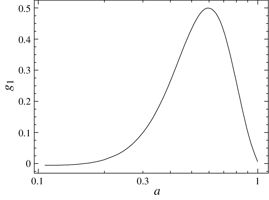
More specifically, let us define a continuous function $V_{1}$ which is the high $N_{p}$ limit of the discrete eigenmode

$$V_{1}(\ln a_{i})\propto S_{i1}\,,$$

(49)

normalized so that

$$\int d\ln aV_{1}^{2}=1\,.$$

(50)

The metric ratio $g$ that this mode represents is given by

$$g_{1}(\ln a)=\left({\rho_{e}\over\rho_{T}}{\Omega_{T}\over\Omega_{e}}\right)^{1/2}V_{1}(\ln a)$$

(51)

and is shown in Fig. 6. Note that the maximum value attained in this function is $g_{\rm max}=0.5$ at a redshift of $z_{\rm max}=0.68$. The ISW effect thus constrains a weighted average of $g$ around $z_{\rm max}$. The falloff in sensitivity near the present epoch is due to projection effects.

We now use this functional form of $g$ to evaluate the WMAP constraint on the amplitude $g_{\rm eff}$

$$g_{\rm SH}(\ln a)={g_{\rm eff}{g_{1}(\ln a)\over g_{\rm max}}}\,.$$

(52)

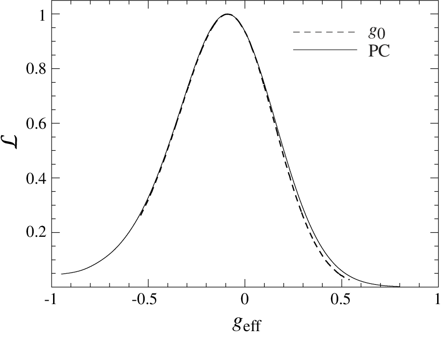
Fig. 7 shows that the posterior probability distribution of $g_{\rm eff}$ is nearly Gaussian and that

$$g_{\rm eff}=-0.12\pm 0.27\,.$$

(53)

Note that $g_{\rm eff}$ is the value of $g_{\rm SH}$ at the $z_{\rm max}$.

Given a specific model for $g$, this constraint should be interpreted as one on a given weighted average of $g$ around $z_{\rm max}$; specifically

$$g_{\rm eff}=g_{\rm max}\int d\ln ap(\ln a)V_{1}(\ln a)\,.$$

(54)

For example, employing the model of Eqn. (44) we obtain $g_{\rm eff}=0.54g_{0}$. In Fig. 7 we show that the direct constraints on $g_{0}$ compare well with those inferred from $g_{\rm eff}$.

The constraints obtained in the previous section are fairly general in that a model that violates them while maintaining the underlying assumptions of a smooth initial power spectrum and an expansion history close to $\Lambda$CDM will be disfavored by the data. However there remains a wide range of interesting phenomenology associated with acceptable models and a weakening of the underlying assumptions.

As an example of phenomenology that PPF models can produce that is not possible in $\Lambda$CDM, consider the statistical curiosity of the low quadrupole power in the CMB. Figure 8 shows that in the maximum likelihood $\Lambda$CDM model, the observed quadrupole is near the $95\%$ cosmic variance limit. A quadrupole realization as extreme as the WMAP data only occurs in $\sim 5.5$% of the time. Of course in the first say 100 multipoles one expects and finds a few such events. The quadrupole is only special because it represents the largest observable scale and may hint at new physics beyond the standard cosmological model.

Construction of a model that sharply lowers the power in the quadrupole but not the octopole is hindered by the fact that in $\Lambda$CDM it gets nearly equal contributions from the ISW effect and the Sachs-Wolfe effect. These contributions are separated by a decade in physical scale making it difficult to invoke initial conditions as an explanation of the low quadrupole [33]. Furthermore for dynamical dark energy models based on scalar fields, it is difficult to reduce the ISW effect while maintaining an expansion history close to $\Lambda$CDM [35, 34].

As we have seen, a modified gravity model can alter the evolution of the metric even for an expansion history that is indistinguishable from $\Lambda$CDM. Let us then construct a model which nearly eliminates the ISW effect at low multipoles while leaving the spectrum at $\ell\gtrsim 10$ unchanged. To enhance the impact on the low multipoles let us take $c_{\Gamma}=0.1$, $c_{g}<0.01$ and take a very steep evolution of $g$ such that deviations appear only recently

$\displaystyle g_{\rm SH}(\ln a)=A\left({\rho_{e}\over\rho_{T}}{\Omega_{T}\over\Omega_{e}}\right)^{2}\,.$

(55)

We find that $A=-0.7$ causes a growth at late times that nearly offsets the earlier decay leaving the ISW effect nearly absent in the quadrupole. Because of the steep evolution, this model evades the constraints from the previous section. We show the spectrum of this model in Fig. 8 (dashed line). This model is a better fit to the WMAP data with a $\Delta 2\ln L=-1.5$. Of course given the number of parameters and ad hoc assumptions of this model, such an improvement is not statistically significant. On the other hand, explorations of this sort can suggest what types of modified gravity models would be fruitful to study: in this case, models with $g<0$ on the horizon scale near the present.

With the ISW effect nearly eliminated the quadrupole can be further lowered by a change in the initial power spectrum of Eqn. (45). Placing a cutoff of $k_{\rm min}=2.4\times 10^{-4}$ Mpc^-1 produces the spectrum shown in Fig. 8 and an improved likelihood of $\Delta 2\ln L=-2.8$.

This example also highlights the primary caveat of applying the constraint on $g_{\rm eff}$ in the previous section. That constraint assumes a featureless initial power spectrum where the constraints at high $\ell$ nearly fix the initial power at the horizon scale today. While this is reasonable given the expectation that gravity is only modified at late times, it remains an assumption nonetheless.

We have generalized the parametrized post-Friedmann (PPF) description of cosmic acceleration from modified gravity to include multiple relativistic matter species and spatial curvature. This generalization facilitates the adaptation of Einstein-Boltzmann codes for modified gravity. We have adapted a comoving gauge code to study constraints on deviations from general relativity on the largest scales through the CMB.

The integrated Sachs-Wolfe (ISW) effect probes the evolution of the metric $\Phi_{-}$ on scales near the horizon during the acceleration epoch. Under the PPF parametrization, modifications to gravity can change the amplitude and shape of the ISW contributions to the low multipole CMB temperature power spectrum even if the expansion history is indistinguishable from that of a cosmological constant. For example in some regions of parameter space, the ISW effect can be nearly eliminated at the quadrupole bringing the predicted ensemble average quadrupole nearer to its observed value on our sky.

We use the WMAP data to constrain such modifications and find that deviations in the metric ratio parameter $g$ are constrained at the level of $g_{\rm eff}=-0.12\pm 0.27$ at $z\sim 0.7$ and $k\sim 10^{-3}$ Mpc^-1. Correspondingly, specific models such as the DGP and some $f(R)$ models are constrained by the data at levels consistent with the findings of previous work (e.g. [18, 20]). By phrasing these and other constraints in the model-independent PPF description, we gain a more general understanding of what aspects of general relativity are tested by the observations.

The modified gravity framework studied here should also enable future studies of other cosmological observables on large scales that are beyond the scope of this work such as the lensing of the CMB and faint galaxies as well as CMB-galaxy correlations.

References

- [1] M. Ishak, A. Upadhye, and D. N. Spergel, Phys. Rev. D74, 043513 (2006), eprint astro-ph/0507184.
- [2] L. Knox, Y.-S. Song, and J. A. Tyson, Phys. Rev. D74, 023512 (2006).
- [3] S. Wang, L. Hui, M. May, and Z. Haiman (2007), eprint arXiv:0705.0165 [astro-ph].
- [4] Y.-S. Song (2006), eprint astro-ph/0602598.
- [5] D. Huterer and E. V. Linder, Phys. Rev. D75, 023519 (2007), eprint astro-ph/0608681.
- [6] R. Caldwell, A. Cooray, and A. Melchiorri, Phys. Rev. D76, 023507 (2007), eprint astro-ph/0703375.
- [7] L. Amendola, M. Kunz, and D. Sapone (2007), eprint arXiv:0704.2421 [astro-ph].
- [8] P. Zhang, M. Liguori, R. Bean, and S. Dodelson, ArXiv e-prints 704 (2007), eprint 0704.1932.
- [9] M. A. Amin, R. V. Wagoner, and R. D. Blandford (2007), eprint arXiv:0708.1793 [astro-ph].
- [10] B. Jain and P. Zhang (2007), eprint arXiv:0709.2375 [astro-ph].
- [11] W. Hu and I. Sawicki, Phys. Rev. D76, 104043 (2007), eprint arXiv:0708.1190 [astro-ph].
- [12] G. R. Dvali, G. Gabadadze, and M. Porrati, Phys. Lett. B485, 208 (2000), eprint hep-th/0005016.
- [13] S. M. Carroll, V. Duvvuri, M. Trodden, and M. S. Turner, Phys. Rev. D70, 043528 (2004), eprint astro-ph/0306438.
- [14] S. Nojiri and S. D. Odintsov, Phys. Rev. D68, 123512 (2003), eprint hep-th/0307288.
- [15] S. Capozziello, S. Carloni, and A. Troisi (2003), eprint astro-ph/0303041.
- [16] U. Seljak and M. Zaldarriaga, Astrophys. J. 469, 437 (1996), eprint astro-ph/9603033.
- [17] A. Lewis, A. Challinor, and A. Lasenby, Astrophys. J. 538, 473 (2000), eprint astro-ph/9911177.
- [18] Y. Song, I. Sawicki, and W. Hu, Phys. Rev. D 75, 064003 (2006), eprint astro-ph/0606286.
- [19] A. Lue, R. Scoccimarro, and G. D. Starkman, Phys. Rev. D69, 124015 (2004), eprint astro-ph/0401515.
- [20] Y. Song, H. Peiris, and W. Hu, Phys. Rev. D 76, 063517 (2007), eprint 0706.2399 [astro-ph].
- [21] F. Schmidt, M. Liguori, and S. Dodelson, Phys. Rev. D76, 083518 (2007), eprint arXiv:0706.1775 [astro-ph].
- [22] L. Pogosian and A. Silvestri, Phys. Rev. D77, 023503 (2008), eprint 0709.0296.
- [23] M. Kunz and D. Sapone, Phys. Rev. Lett. 98, 121301 (2007), eprint astro-ph/0612452.
- [24] S. Bashinsky (2007), eprint arXiv:0707.0692 [astro-ph].
- [25] W. Hu, Astrophys. J. 506, 485 (1998), eprint astro-ph/9801234.
- [26] J. M. Bardeen, Phys. Rev. D 22, 1882 (1980).
- [27] H. Kodama and M. Sasaki, Prog. Theor. Phys. Suppl. 78, 1 (1984).
- [28] W. Hu and D. J. Eisenstein, Phys. Rev. D 59, 083509 (1999), eprint astro-ph/9809368.
- [29] E. Bertschinger, Astrophys. J. 648, 797 (2006), eprint astro-ph/0604485.
- [30] W. Hu and T. Okamoto, Phys. Rev. D 69, 043004 (2003), eprint astro-ph/0308049.
- [31] W. Hu, U. Seljak, M. White, and M. Zaldarriaga, Phys. Rev. D 57, 3290 (1998), eprint astro-ph/9709066.
- [32] D. N. Spergel et al. (WMAP), Astrophys. J. Suppl. 170, 377 (2007), eprint astro-ph/0603449.
- [33] C. Contaldi, M. Peloso, L. Kofman, and A. Linde, JCAP 0307, 002 (2003), eprint astro-ph/0303636.
- [34] C. Gordon and W. Hu, Phys. Rev. D 70, 083003 (2004), eprint astro-ph/0406496.
- [35] R. Bean and O. Dore, Phys. Rev. D 69, 083503 (2004), eprint astro-ph/0307100.