The Keldysh action of a multi-terminal time-dependent scatterer.

I. Snyman Affiliation: Instituut-Lorentz, Universiteit Leiden, P.O. Box 9506, 2300 RA Leiden, The Netherlands Y.V. Nazarov Affiliation: Kavli Institute of Nanoscience, Delft University of Technology, 2628 CJ Delft, The Netherlands

August 24, 2026

Abstract

We present a derivation of the Keldysh action of a general multi-channel time-dependent scatterer in the context of the Landauer-Büttiker approach. The action is a convenient building block in the theory of quantum transport. This action is shown to take a compact form that only involves the scattering matrix and reservoir Green functions. We derive two special cases of the general result, one valid when reservoirs are characterized by well-defined filling factors, the other when the scatterer connects two reservoirs. We illustrate its use by considering Full Counting Statistics and the Fermi Edge Singularity.

pacs

73.23.-b, 73.50.Td, 05.40.-a

I Introduction

The pioneering work of Landauer[1, 2] and Büttiker[3, 4] lay the foundations for what is now known as the scattering approach to electron transport. The basic tenet is that a coherent conductor is characterized by its scattering matrix. More precisely the transmission matrix defines a set of transparencies for the various channels or modes in which the electrons propagate through the conductor. As a consequence, conductance is the sum over transmission probabilities. Subsequently, it was discovered that the same transmission probabilities fully determine the current noise, also outside equilibrium, where the fluctuation-dissipation theorem does not hold[5].

Indeed, as the theory of Full Counting Statistics [6, 7, 8] later revealed, the complete probability distribution for outcomes of a current measurement is entirely characterized by the transmission probabilities of the conductor. The fact that the scattering formalism gives such an elegant and complete description inspired some to revisit established results. Thus for instance interacting problems such as the Fermi Edge Singularity [9, 10] was recast in the language of the scattering approach[11, 12, 13, 14]. The scattering approach has further been employed successfully in problems where a coherent conductor interacts with other elements, including, but not restricted to, measuring devices and an electromagnetic environment [15, 16, 17, 18]. It is also widely applied to study transport in mesoscopic superconductors [19].

Many of these more advanced applications are unified through a method developed by Feynman and Vernon for characterizing the effect of one quantum system on another when they are coupled [20]. The work of Feynman and Vernon dealt with the effect of a bath of oscillators coupled to a quantum system. It introduced the concept of a time-contour describing propagation first forwards then backwards in time. By using the path-integral formalism, it was possible to characterize the bath by an “influence functional” that did not depend on the system that the bath was coupled to. This functional was treated non-perturbatively. A related development was due to Keldysh [21]. While being a perturbative diagrammatic technique, it allowed for the treatment of general systems and shared the idea of a forward and backward time-contour with Feynman and Vernon. Applications involving the scattering approach require both the notion of the non-perturbative influence functional and the generality of Keldysh’s formalism. Until now, the combination of the Feynman-Vernon method with the scattering approach was done on an case-specific basis. Only those elements relevant to the particular application under consideration were developed. In this paper we unify previous developments by deriving general formulas for the influence functional, or equivalently the Keldysh action of a general scatterer connected to charge reservoirs.

The Keldysh action of a general scatterer can be considered as a building block. Its “interface” is the set of fields $\chi_{\pm}(t)$ . Through this interface, the actions of many conductors can be combined into quantum circuits. As in the case of classical electronics, a simple set of rules, applied at the nodes of such a circuit, suffice to describe the behavior of the whole network [23, 24].

The influence functional $\mathcal{Z}[\chi_{\pm}]$ and the Keldysh action $\mathcal{A}[\chi_{\pm}]=\ln\mathcal{Z}[\chi_{\pm}]$ depend on two sets of time-dependent fields $\chi_{+}(t)$ and $\chi_{-}(t)$ corresponding to forward and backward evolution in time with different Hamiltonians. Recently, the situation was considered where $\chi_{\pm}$ are time-independent but the scatterer was allowed to fluctuate in time [22]. We consider the case where also the fields $\chi_{\pm}$ are time-dependent. Functional derivatives with respect to these fields generate cumulants of the distribution of outcomes for the measurement of the degrees of freedom coupled to $\chi_{\pm}$ . Since these fields enter the Hamiltonian of the scatterer as a time-dependent potential energy term, their effect is captured by the scattering matrix. Since the fields differ for forward and backward evolution, the scattering matrices for forward and backward evolution differ.

Our main result is summarized by a formula for this Keldysh action.

\mathcal{A}[\hat{s}]={\rm Tr\;ln}\left[\frac{1+\hat{G}}{2}+\hat{s}\frac{1-\hat{G}}{2}\right]-{\rm Tr\;ln}\;\hat{s}_{-}.

(1)

In this formula, $\hat{G}$ is the Keldysh Green function characterizing the reservoirs connected to the scatterer [25]. It is to be viewed as an operator with kernel $G(\alpha,\alpha^{\prime};c;t,t^{\prime})\delta_{c,c^{\prime}}$ where the Keldysh indices $\alpha,\,\alpha^{\prime}\in\{+,-\}$ refer to time-contour ordering, $c,\,c^{\prime}\in Z$ refer to channel space, and $t,\,t^{\prime}\in R$ are continuous time indices. The dependence on the fields $\chi_{\pm}$ is carried by the time-dependent scattering matrix $\hat{s}$ , that also has Keldysh structure, owing to forward and backward time-evolution with different Hamiltonians. Explicitly, it is to be viewed as an operator with kernel $s(\alpha;c,c^{\prime};t)\delta_{\alpha,\alpha^{\prime}}\delta(t-t^{\prime})$ where indices carry the same meaning as in the kernel of $\hat{G}$ . This formula is completely general.

1.

It holds for multi-terminal devices with more than two reservoirs.
2.

It holds for devices such as Hall bars where particles in a single chiral channel enter and leave the conductor at different reservoirs.
3.

It holds when reservoirs cannot be characterized by stationary filling factors. Reservoirs may be superconducting, or contain “counting fields” coupling them to a dynamical electromagnetic environment or a measuring device.

When the reservoirs can indeed be characterized by filling factors $\hat{f}(\varepsilon)$ , the Keldysh structure can explicitly be traced out to yield

\mathcal{A}[\hat{s}_{+},\hat{s}_{-}]={\rm Tr\;ln}\left[\hat{s}_{-}(1-\hat{f})+\hat{s}_{+}\hat{f}\right]-{\rm Tr\;ln}\;\hat{s}_{-}.

(2)

In this expression operators retain channel structure and time structure. The time-dependent scattering matrices $\hat{s}_{\pm}$ have kernels $s_{\pm}(c,c^{\prime};t)\delta(t-t^{\prime})$ that depend on the field $\chi_{\pm}(t)$ . In “time” representation, $\hat{f}$ is the Fourier transform to time of the reservoir filling factors, and as such has a kernel $f(c;t,t^{\prime})\delta_{c,c^{\prime}}$ diagonal in channel space and depending on two times. This formula is of the same type as the Levitov-Lesovik formula for zero frequency Full Counting Statistics (FCS) [8], but contains information about finite frequencies due to the arbitrary time-dependence of $\hat{s}_{\pm}$ .

Another formula may be derived from Eq. (1), valid for two terminal devices. Each terminal may still be connected to the scatterer by an arbitrary number of channels. We denote the two terminals left (L) and right (R). In this case the reservoir Green function has the form

\hat{G}=\left(\begin{array}[]{cc}\check{G}_{L}&0\\ 0&\check{G}_{R}\end{array}\right)_{\rm channel\,space}

(3)

where $\check{G}_{L(R)}$ have no further channel space structure. Matrix structure in Keldysh and time indices (indicated by a check sign) is now retained in the trace, but the channel structure is traced out. Thus is obtained

\mathcal{A}[\chi_{\pm}]=\frac{1}{2}\sum_{n}{\rm Tr}\,{\rm ln}\left[1+T_{n}\frac{\left\{\check{G}_{L}[\chi_{\pm}],\check{G}_{R}[\chi_{\pm}]\right\}-2}{4}\right].

(4)

In this expression, the field dependence $\chi_{\pm}$ is shifted to the Keldysh Green functions $\check{G}_{L}$ and $\check{G}_{R}$ of the left and right reservoirs. This formula makes it explicit that the conductor is completely characterized by its transmission eigenvalues $T_{n}$ .

The plan of the text is as follows. After making the necessary definitions, we derive Eq. (1) from a model Hamiltonian. The derivation makes use of contour ordered Green functions and the Keldysh technique. Subsequently, we derive the special cases of Eq. (2) and Eq. (4). While the formulas (2) and (4) have appeared in the literature before, as far as we know, there has not yet appeared a formal derivation.

We conclude by applying the formulas to several generic set-ups, and verify that results agree with the existing literature. Particularly, we explain in detail how the present work is connected to the theory of Full Counting Statistics and to the scattering theory of the Fermi Edge Singularity.

II Derivation

Refer to caption — Figure 1: We consider a general scatterer connected to reservoirs. The top figure is a diagram of one possible physical realization of a scatterer. Channels carry electrons towards and away from a scattering region (shaded dark gray) where inter-channel scattering takes place. Reservoirs are characterized by Keldysh Green functions $G_{\rm in\,(out)}$ . These Green functions also carry a channel index, in order to account for, among other things, voltage biasing. In setups such as the the Quantum Hall experiment where there is a Hall voltage, $G_{\rm in}$ will differ from $G_{\rm out}$ , while in an ordinary QPC, the two will be identical. The bottom figure shows how the physical setup is represented in our model. Channels are unfolded so that all electrons enter at $z^{-}$ and leave at $z^{+}$ .

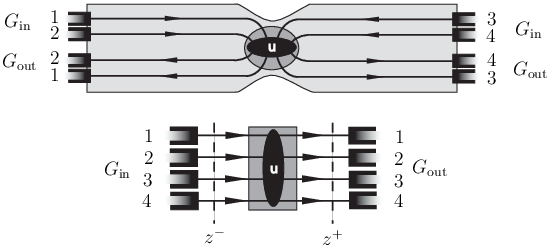
We consider a general scatterer connecting a set of charge reservoirs. We allow the scatterer to be time-dependent. A sufficient theoretical description is provided by set of transport channels interrupted by a potential that causes inter-channel scattering. We consider the regime where the scattering matrix is energy-independent in the transport energy window. Since transport is purely determined by the scattering matrix, all models that produce the same scattering matrix give identical results. Regardless of actual microscopic detail, we may therefore conveniently take the Hamiltonian of the scatterer to be

	$\displaystyle\mathcal{H}=$	$\displaystyle v_{F}\sum_{m,n}\int dz\;\psi^{\dagger}_{m}(z)\left\{-i\delta_{m,n}\partial_{z}+u_{m,n}(z)\right\}\psi_{n}(z)$
		$\displaystyle+\mathcal{H}_{\rm res}+\mathcal{H}_{\rm T},$		(5)

where $\mathcal{H}_{\rm res}$ represents the reservoirs, and $\mathcal{H}_{\rm T}$ takes account of tunneling between the conductor and the reservoirs. The scattering region and the reservoirs are spatially separated. This means that the scattering potential $u_{mn}(z)$ is non-zero only in a region $z^{-}<z<z^{+}$ while tunneling between the reservoirs and the conductor only takes place outside this region. Note that in our model, scattering channels have been “unfolded”, so that in stead of working with a channel that confines particles in the interval $(-\infty,0]$ and allowing for propagation both in the positive and negative directions, we equivalently work with channels in which particles propagate along $(-\infty,\infty)$ , but only in the positive direction. Hence, to make contact with most physical setups, we consider $-z$ and $z$ to refer to the same physical position in a channel, but opposite propagation directions.

We consider the generating functional

\mathcal{Z}=e^{\mathcal{A}}={\rm Tr}\left[\mathcal{T}^{+}\exp\left\{-i\int_{t_{0}}^{t_{1}}dt\;\mathcal{H}^{+}(t)\right\}\rho_{0}\mathcal{T}^{-}\exp\left\{i\int_{t_{0}}^{t_{1}}dt\;\mathcal{H}^{-}(t)\right\}\right]

(6)

in which $\mathcal{H}^{\pm}$ is obtained from $\mathcal{H}$ by replacing $u_{mn}(z)$ with arbitrary time-dependent functions $u^{\pm}_{mn}(z,t)$ . In this expressions $\mathcal{T}^{+}\exp$ and $\mathcal{T}^{-}\exp$ respectively refer to time-ordered (i.e. largest time to the left) and anti-time-ordered (i.e. largest time to the right) exponentials. In the language of Feynman end Vernon [20] this is known as the influence functional. It gives a complete characterization of the effect that the electrons in the scatterer have on any quantum system that interact with. Furthermore, the functional $\mathcal{Z}$ generates expectation values of time-ordered products of operators as follows. Let $Q$ be an operator

Q=\sum_{mn}\int_{z^{-}}^{z^{+}}dz\,\psi_{m}^{\dagger}(z)q_{mn}(z)\psi_{n}(z).

(7)

Choose $u^{\pm}_{mn}(z,t)=u_{mn}(z)+\chi_{\pm}(t)q_{mn}(z)$ . Then

		$\displaystyle\left<\mathcal{T}^{-}\left(\prod_{j=1}^{M}Q(t_{j})\right)\mathcal{T}^{+}\left(\prod_{k=1}^{N}Q(t_{k}^{\prime})\right)\right>$
		$\displaystyle=\prod_{j=1}^{M}\left(-i\frac{\delta}{\delta\chi^{-}(t_{j})}\right)\prod_{k=1}^{N}\left(i\frac{\delta}{\delta\chi^{+}(t_{k}^{\prime})}\right)\left.\mathcal{Z}[\chi]\right\|_{\chi=0}$		(8)

By merging the power of the Keldysh formalism of contour-ordered Green functions with that of the Landauer scattering formalism for quantum transport, we obtain an expression for $\mathcal{Z}$ in terms of the Keldysh Green functions in the reservoirs and the time dependent scattering matrices associated with $\hat{u}^{\pm}(z,t)$ .

The argument will proceed in the following steps:

1.

Firstly we introduce the key object that enables a systematic analysis of $\mathcal{Z}$ , namely the single particle Green function $g$ of the conductor. We state the equations of motion that $g$ obeys.
2.

We define the Keldysh action $\mathcal{A}=\ln\mathcal{Z}$ , and consider its variation $\delta\mathcal{A}$ . We discover that $\delta\mathcal{A}$ can be expressed in terms of $g$ .
3.

We therefore determine $g$ inside the scattering region in terms of the scattering matrix of the conductor and its value at the edges of the scattering region, where the reservoirs impose boundary conditions.
4.

This allows us to express the variation of the action in terms of the reservoir Green functions $G_{\rm in\,(out)}$ and the scattering matrix $s$ of the conductor.
5.

The variation $\delta\mathcal{A}$ is then integrated to find the action $\mathcal{A}$ and the generating functional $\mathcal{Z}$ .

II.1 Preliminaries: Definition of the Green function

The first step is to move from the Schrödinger picture to the Heisenberg picture. To shorten notation we define two time-evolution operators:

\mathcal{U}_{\pm}(t_{f},t_{i})=\mathcal{T}^{+}\exp\left\{-i\int_{t_{i}}^{t_{f}}dt^{\prime}\;\mathcal{H}^{\pm}(t^{\prime})\right\}.

(9)

Associated with every Schrödinger picture operator we define two Heisenberg operators, one corresponding to evolution with each of the two Hamiltonians $\mathcal{H}^{\pm}$ .

Q_{\pm}(t)=\mathcal{U}_{\pm}(t_{f},t_{i})^{\dagger}\,Q\,\mathcal{U}_{\pm}(t_{f},t_{i}).

(10)

In order to have the tools of the Keldysh formalism at our disposal, we need to define four Green functions

$\displaystyle g_{m,n}^{++}(z,t;z^{\prime},t^{\prime})$	$\displaystyle=$	$\displaystyle-e^{\mathcal{A}}{\rm Tr}\left[\mathcal{U}^{+}(t_{1},t_{0})\mathcal{T}^{+}\left(\psi_{n+}^{\dagger}(z^{\prime},t^{\prime})\psi_{m+}(z,t)\right)\rho_{0}\left(\mathcal{U}^{-}(t_{1},t_{0})\right)^{\dagger}\right]$
$\displaystyle g_{m,n}^{+-}(z,t;z^{\prime},t^{\prime})$	$\displaystyle=$	$\displaystyle e^{\mathcal{A}}{\rm Tr}\left[\mathcal{U}^{+}(t_{1},t_{0})\psi_{m+}(z,t)\rho_{0}\psi^{\dagger}_{n-}(z^{\prime},t^{\prime})\left(\mathcal{U}^{-}(t_{1},t_{0})\right)^{\dagger}\right]$
$\displaystyle g_{m,n}^{-+}(z,t;z^{\prime},t^{\prime})$	$\displaystyle=$	$\displaystyle e^{\mathcal{A}}{\rm Tr}\left[\mathcal{U}^{+}(t_{1},t_{0})\psi_{n+}^{\dagger}(z^{\prime},t^{\prime})\rho_{0}\psi_{m-}(z,t)\left(\mathcal{U}^{-}(t_{1},t_{0})\right)^{\dagger}\right]$
$\displaystyle g_{m,n}^{--}(z,t;z^{\prime},t^{\prime})$	$\displaystyle=$	$\displaystyle e^{\mathcal{A}}{\rm Tr}\left[\mathcal{U}^{+}(t_{1},t_{0})\rho_{0}\mathcal{T}^{-}\left(\psi_{n-}^{\dagger}(z^{\prime},t^{\prime})\psi_{m-}(z,t)\right)\left(\mathcal{U}^{-}(t_{1},t_{0})\right)^{\dagger}\right].$	(11)

Here the symbol $\mathcal{T}^{+}$ orders operators with larger time arguments to the left. If permutation is required to obtain the time-ordered form, the product is multiplied with $(-1)^{n}$ where $n$ is the parity of the permutation. Similarly, $\mathcal{T}^{-}$ anti-time-orders with the same permutation parity convention.

The Green functions can be grouped into a matrix in Keldysh space

g_{m,n}(z,t;z^{\prime},t^{\prime})=\left(\begin{array}[]{cc}g^{++}_{m,n}(z,t;z^{\prime},t^{\prime})&g^{+-}_{m,n}(z,t;z^{\prime},t^{\prime})\\ g^{-+}_{m,n}(z,t;z^{\prime},t^{\prime})&g^{--}_{m,n}(z,t;z^{\prime},t^{\prime})\end{array}\right).

(12)

Notation can be further shortened by incorporating channel-indices into the matrix structure of the Green function, thereby defining an object $\bar{g}(z,t;z^{\prime},t^{\prime})$ . The element of $\bar{g}$ that is located on row $m$ and column $n$ , is the $2\times 2$ matrix $g_{m,n}$ .

The Green function satisfies the equation of motion

		$\displaystyle\left\{i\partial_{t}+v_{F}i\partial_{z}-v_{F}\bar{u}(z,t)\right\}\bar{g}(z,t;z^{\prime},t^{\prime})$
		$\displaystyle-\int dt^{\prime\prime}\Sigma(z;t-t^{\prime\prime})\bar{g}(z,t^{\prime\prime};z^{\prime}t^{\prime})=\delta(t-t^{\prime})\delta(z-z^{\prime})\bar{1}.$		(13)

The delta-functions on the right of Eq. (13) encode the fact that due to time-ordering $g_{mn}^{++}$ and $g_{mn}^{--}$ have a step-structure

\frac{1}{v_{F}}\theta(z-z^{\prime})\delta(t-t^{\prime}-\frac{z-z^{\prime}}{v_{F}})\delta_{mn}+f(z,t;z^{\prime}t^{\prime})

(14)

where $f$ is continuous in all its arguments. The self-energy

\Sigma(z;\tau)=-i\frac{\bar{G}_{\rm in}(\tau)}{2\tau_{c}}\theta(z^{-}-z)-i\frac{\bar{G}_{\rm out}(\tau)}{2\tau_{c}}\theta(z-z^{+})

(15)

results from the reservoirs and determines how the scattering channels are filled. It is a matrix in Keldysh space. The time $\tau_{c}$ is the characteristic time correlations survive in the region of the conductor that is connected to the reservoirs, before the reservoirs scramble them. $\bar{G}_{\rm in\,(out)}(\tau)$ is the reservoir Green functions where electrons enter (leave) the scattering region, summed over reservoir levels and normalized to be dimensionless. This form of the self-energy can be derived from the following model for the reservoirs: We imagine every point $z$ in a channel $m$ outside $(z^{-},z^{+})$ to exchange electrons with an independent Fermion bath with a constant density of states $\nu$ . The terms $\mathcal{H}_{\rm res}$ and $\mathcal{H}_{\rm T}$ are explicitly

$\displaystyle\mathcal{H}_{\rm res}$	$\displaystyle=$	$\displaystyle\sum_{m}\int dE\,\nu\,\int_{z\not\in(z^{-},z^{+})}dz\,E\,a_{m}^{\dagger}(E,z)a_{m}(E,z)$
$\displaystyle\mathcal{H}_{\rm T}$	$\displaystyle=$	$\displaystyle\sum_{m}\,c_{m}\int dE\,\nu\,\int_{z\not\in(z^{-},z^{+})}dz\,\psi^{\dagger}_{m}(z)a_{m}(E,z)$	(16)
		$\displaystyle\hskip 14.22636pt+a^{\dagger}_{m}(E,z)\psi_{m}(z),$	(16)

where the tunneling amplitude $c_{m}$ characterizes the coupling between the reservoir and channel $m$ . More general reservoir models need not be considered, since, as we shall see shortly, the effect of the reservoirs is contained entirely in a boundary conditions on the Green function $\bar{g}$ inside the scatterer. This boundary condition does not depend on microscopic detail, but only on the reservoir Green functions $\bar{G}_{\rm in\,(out)}$ .

We do not need to know the explicit form of the reservoir Green functions yet. Rather the argument below relies exclusively on the property of $\bar{G}_{\rm in\,(out)}$ that it squares to unity [25]:

\int dt^{\prime\prime}\,\bar{G}(t-t^{\prime\prime})_{\rm in\,(out)}\bar{G}(t^{\prime\prime}-t^{\prime})_{\rm in\,(out)}=\delta(t-t^{\prime})\bar{1}.

(17)

A differential equation similar to Eq. (13) holds for $\bar{g}^{\dagger}$ .

II.2 Varying the action $\mathcal{A}$ .

We are now ready to attack the generating functional $\mathcal{Z}$ . For our purposes, it is most convenient to consider $\mathcal{A}=\rm ln\,\mathcal{Z}$ . We will call this object the action. Our strategy is as follows: We will obtain an expression for the variation $\delta\mathcal{A}$ resulting from a variation $\hat{u}(z,t)\to\hat{u}(z,t)+\delta\hat{u}(z,t)$ of the scattering potentials. This expression will be in terms of the reservoir filling factors $\hat{f}$ and the scattering matrices associated with $\hat{u}(z,t)$ . We then integrate to find $\mathcal{A}$ .

We start by writing

\delta\mathcal{A}=-iv_{F}e^{\mathcal{A}}\sum_{m,n}\int_{t_{0}}^{t_{1}}dt\int dz\;\left(\delta u^{+}_{n,m}(z,t)\left<\psi_{m}^{\dagger}(z)\psi_{n}(z)\right>_{+}(t)-\delta u^{-}_{n,m}(z,t)\left<\psi_{m}^{\dagger}(z)\psi_{n}(z)\right>_{-}(t)\right)

(18)

where

$\displaystyle\left<\psi_{m}^{\dagger}(z)\psi_{n}(z)\right>_{+}(t)$
	$\displaystyle=$	$\displaystyle{\rm Tr}\left[\mathcal{T}^{+}\exp\left\{-i\int_{t}^{t_{1}}dt^{\prime}\;\mathcal{H}^{+}(t^{\prime})\right\}\psi_{m}^{\dagger}(z)\psi_{n}(z)\mathcal{T}^{+}\exp\left\{-i\int_{t_{0}}^{t}dt^{\prime}\;\mathcal{H}^{+}(t^{\prime})\right\}\rho_{0}\mathcal{T}^{-}\exp\left\{i\int_{t_{0}}^{t_{1}}dt^{\prime}\;\mathcal{H}^{-}(t^{\prime})\right\}\right]$
$\displaystyle\left<\psi_{m}^{\dagger}(z)\psi_{n}(z)\right>_{-}(t)$
	$\displaystyle=$	$\displaystyle{\rm Tr}\left[\mathcal{T}^{+}\exp\left\{-i\int_{t_{0}}^{t_{1}}dt^{\prime}\;\mathcal{H}^{+}(t^{\prime})\right\}\rho_{0}\mathcal{T}^{-}\exp\left\{i\int_{t_{0}}^{t}dt^{\prime}\;\mathcal{H}^{-}(t^{\prime})\right\}\psi_{m}^{\dagger}(z)\psi_{n}(z)\mathcal{T}^{-}\exp\left\{-i\int_{t}^{t_{1}}dt^{\prime}\;\mathcal{H}^{-}(t^{\prime})\right\}\right].$

II.3 Expressing $\delta\mathcal{A}$ in terms of the Green function $g$ .

In terms of the defined Green functions, the variation $\delta\mathcal{A}$ becomes

$\displaystyle\delta\mathcal{A}$	$\displaystyle=$	$\displaystyle iv_{F}\sum_{m,n}\int_{t_{0}}^{t_{1}}dt\int dz\ \;\Big(\delta u^{+}_{n,m}(z,t)$
		$\displaystyle\hskip 42.67912pt\times g_{m,n}^{++}(z,t-0^{+};z,t)$
		$\displaystyle\hskip 28.45274pt+\delta u^{-}_{n,m}(z,t)g_{m,n}^{--}(z,t+0^{+};z,t)\Big)$
	$\displaystyle=$	$\displaystyle iv_{F}\int_{t_{0}}^{t_{1}}dt\int dz\;{\rm Tr}\left[\delta\bar{u}(z,t)\bar{g}(z,t+0^{k};z,t)\right].$

The object $\delta\bar{u}$ is constructed by combining the channel and Keldysh indices of the variation of the potential. The trace is over both Keldysh and channel indices. The symbol $0^{k}$ refers to the regularization explicitly indicated in the first line, i.e. the first time argument of $g^{++}(z,t-0^{+};z,t)$ is evaluated an infinitesimal time $0^{+}>0$ before the second argument, while in $g^{--}(z,t+0^{-};z,t)$ , the first time argument is evaluated an infinitesimal time $0^{+}$ after the second. This is done so that the time ordering (anti-time ordering) operations give the order of creation and annihilation operators required in Eq. (18).

It proves very inconvenient to deal with the $0^{k}$ regularization of Eq. (). It is preferable to have the first time arguments of both $g^{++}$ and $g^{--}$ evaluated an infinitesimal time $0^{+}$ before the second. Taking into account the step-structure of $\hat{g}^{++}$ we have

		$\displaystyle\bar{g}(z,t+0^{k};z^{\prime}t^{\prime})=\bar{g}(z,t-0^{+};z^{\prime},t^{\prime})$
		$\displaystyle\hskip 14.22636pt+\frac{1}{v_{F}}\delta(t-t^{\prime}-\frac{z-z^{\prime}}{v_{F}})\hat{1}\left(\frac{1-\check{\tau}_{3}}{2}\right).$		(21)

Here $\check{\tau}_{3}$ is the third Pauli matrix $\left(\begin{array}[]{cc}1&0\\ 0&-1\end{array}\right)$ acting in Keldysh space. The equations of motion allow us to relate $\bar{g}(z,t-0^{+};z^{\prime},t^{\prime})$ for points $z$ and $z^{\prime}$ inside the scattering region where $\bar{u}$ is non-zero, to the value of $\bar{g}$ at $z^{-}$ where electrons enter the scatterer. For $z\leq z^{\prime}$ and $t\leq t^{\prime}$ , the equations of motion give

		$\displaystyle\bar{g}(z,t+\frac{z-z^{-}}{v_{F}}-0^{;}z^{\prime},t+\frac{z^{\prime}-z^{-}}{v_{F}})$
		$\displaystyle=\bar{s}(z,t)\bar{g}(z^{-},t-0^{+};z^{\prime-},t^{\prime})\bar{s}^{\dagger}(z^{\prime},t^{\prime}),$		(22)

where

\bar{s}(z,t)=\mathcal{Z}\exp\left\{-i\int_{z^{-}}^{z}dz^{\prime\prime}\bar{u}(z^{\prime\prime},t+\frac{z^{\prime\prime}-z^{-}}{v_{F}})\right\}.

(23)

The symbol $\mathcal{Z}$ indicates that the exponent is ordered along the $z$ -axis, with the largest co-ordinate in the integrand to the left. Note that the potential $\bar{u}$ at position $z$ is evaluated at the time instant $t+(z-z^{-})/v_{F}$ that an electron entering the scattering region at time $t$ reaches $z$ . Often the time-dependence of the potential is slow on the time-scale $(z^{+}-z^{-})/v_{F}$ representing the time a transported electron spends in the scattering region and $\bar{u}(z,t+\frac{z-z^{-}}{v_{F}})$ can be replaced with $\bar{u}(z,t)$ . This is however not required for the analysis that follows to be valid.

Substitution into Eq. (24) yields

	$\displaystyle\delta A=$	$\displaystyle v_{F}\int dt\;{\rm Tr}\left[\bar{w}(t)g(z^{-},t-0^{+};z^{-},t)\right]$
		$\displaystyle-\int dt\;\lim_{t^{\prime}\rightarrow t}\delta(t-t^{\prime}){\rm Tr}\;\left[\bar{w}(t)\hat{1}\left(\frac{1-\check{\tau}_{3}}{2}\right)\right].$		(24)

with

	$\displaystyle\bar{w}(t)$	$\displaystyle=$	$\displaystyle-i\int_{z^{-}}^{z^{+}}dz\bar{s}^{\dagger}(z,t)\delta\bar{u}(z,t+\frac{z-z^{-}}{v_{F}})\bar{s}(z,t)$		(25)
		$\displaystyle=$	$\displaystyle\bar{s}^{\dagger}(t)\delta\bar{s}(t).$		(25)

In this equation $z^{+}$ is located where electrons leave the scatterer. Importantly, here $\rm Tr$ still denotes a trace over channel and Keldysh indices. We will later on redefine the symbol to include also a trace over the (continuous) time index, at which point the second term in Eq. (24) will (perhaps deceptively) look less offensive, but not yet. In the last line of Eq. (25), $\bar{s}(t)=\bar{s}(z^{+},t)$ is the (time-dependent) scattering matrix. We sent the boundaries $t_{0}$ and $t_{1}$ over which we integrate in the definition of the action, to $-\infty$ and $\infty$ respectively, which will allow us to Fourier transform to frequency in a moment. The action remains well-defined as long as the potentials $u^{+}$ and $u^{-}$ only differ for a finite time.

II.4 Relating $g$ inside the scattering region to $g$ at reservoirs. Imposing boundary conditions implied by reservoirs.

Our task is now to find $\bar{g}(z^{-},t-0^{+};z^{-},t)$ . Because of the $t-t^{\prime}$ dependence of the self-energy, it is convenient to transform to Fourier space, where

	$\displaystyle\bar{g}(z,\varepsilon;z^{-},\varepsilon^{\prime})$	$\displaystyle=$	$\displaystyle\int dt\,dt^{\prime}\,e^{i\varepsilon t}\bar{g}(z,t;z^{-},t^{\prime})e^{-i\varepsilon^{\prime}t^{\prime}}$
	$\displaystyle\bar{G}_{\rm in\,(out)}(\varepsilon)$	$\displaystyle=$	$\displaystyle\int dt\;e^{i\varepsilon t}\bar{G}(t)_{\rm in\,(out)}.$		(26)

In frequency domain, the property that $\bar{G}_{\rm in\,(out)}$ squares to unity is expressed as $\bar{G}_{\rm in\,(out)}(\varepsilon)^{2}=\bar{1}$ . (Due to the standard conventions for Fourier transforms, the matrix elements of the identity operator in energy domain is $2\pi\delta(\varepsilon-\varepsilon^{\prime})$ .) The equation of motion for $z<z^{-}$ reads

\left\{-i\varepsilon+v_{F}\partial_{z}+\frac{\bar{G}_{\rm in}(\varepsilon)}{2\tau_{c}}\right\}\bar{g}(z,\varepsilon;z^{-},\varepsilon^{\prime})=0.

(27)

There is no inhomogeneous term on the right-hand side, because we restrict $z$ to be less than $z^{-}$ . We thus find

		$\displaystyle\bar{g}(z^{-}-0^{+},\varepsilon;z^{-},\varepsilon^{\prime})$
		$\displaystyle=e^{i\varepsilon\Delta z/v_{F}}\exp\left[-\frac{\bar{G}_{\rm in}(\varepsilon)}{2l_{c}}\Delta z\right]\bar{g}(z^{-}-\Delta z,\varepsilon;z^{-},\varepsilon^{\prime}).$		(28)

Here the correlation length $l_{c}$ is the correlation time $\tau_{c}$ multiplied by the Fermi velocity $v_{F}$ . Using the fact that $\bar{G}(\varepsilon)_{\rm in}$ squares to unity, it is easy to verify that

		$\displaystyle\exp\left\{-\frac{\bar{G}_{\rm in}(\varepsilon)}{2l_{c}}\Delta z\right\}$
		$\displaystyle=\frac{1+\bar{G}_{\rm in}(\varepsilon)}{2}\exp\left(-\frac{\Delta z}{2l_{c}}\right)+\frac{1-\bar{G}_{\rm in}(\varepsilon)}{2}\exp\left(\frac{\Delta z}{2l_{c}}\right).$		(29)

Since spacial correlations decay beyond $z^{-}$ , $\bar{g}(z^{-}-\Delta z,\varepsilon;z^{-},\varepsilon^{\prime})$ does not blow up as we make $\Delta z$ larger. From this we derive the condition

\left[1+\bar{G}_{\rm in}(\varepsilon)\right]\bar{g}(z^{-}-0^{+},\varepsilon;z^{-},\varepsilon^{\prime})=0.

(30)

Transformed back to the time-domain this reads

\int dt^{\prime\prime}\;\left[\delta(t-t^{\prime\prime})+\bar{G}_{\rm in}(t-t^{\prime\prime})\right]\bar{g}(z^{-}-0^{+},t^{\prime\prime};z^{-},t^{\prime})=0.

(31)

We can play the same game at $z^{+}$ where particles leave the scatterer. The equation of motion reads

\left\{-i\varepsilon+v_{F}\partial_{z}+\theta(z-z^{+})\frac{\bar{G}_{\rm out}(\varepsilon)}{2\tau_{c}}\right\}\bar{g}(z,\varepsilon;z^{+},\varepsilon^{\prime})=2\pi\delta(z-z^{\prime})\delta(\varepsilon-\varepsilon^{\prime}).

(32)

This has the general solution

	$\displaystyle\bar{g}(z,\varepsilon;z^{\prime},\varepsilon^{\prime})$	$\displaystyle=$	$\displaystyle\exp\left\{i\varepsilon\frac{z-z^{\prime}}{v_{F}}-\left[(z-z^{+})\theta(z-z^{+})-(z^{\prime}-z^{+})\theta(z^{\prime}-z^{+})\right]\frac{\bar{G}_{\rm out}(\varepsilon)}{2l_{c}}\right\}$		(33)
			$\displaystyle\hskip 28.45274pt\times\left[\bar{g}(z^{\prime}-0^{+},\varepsilon^{\prime};z^{\prime},\varepsilon^{\prime})+\frac{2\pi}{v_{F}}\theta(z-z^{\prime})\delta(\varepsilon-\varepsilon^{\prime})\right].$		(33)

We will need to relate the Green function evaluated at $z<z^{+}$ to the Green function evaluated at $z>z^{+}$ , and so we explicitly show the inhomogeneous term. The same kind of argument employed at $z^{-}$ then yields the condition

\left[1-\bar{G}_{\rm out}(\varepsilon)\right]\left[\bar{g}(z^{+}-0^{+},\varepsilon;z^{+},\varepsilon^{\prime})+\frac{2\pi}{v_{F}}\delta(\varepsilon-\varepsilon^{\prime})\right]=0,

(34)

where the inhomogeneous term in the equation of motion is responsible for the delta-function. In time-domain this reads

\int dt^{\prime\prime}\;\left[\delta(t-t^{\prime\prime})-\bar{G}_{\rm out}(t-t^{\prime\prime})\right]\left[\bar{g}(z^{+}-0^{+},t^{\prime\prime};z^{+},t^{\prime})+\frac{1}{v_{F}}\delta(t^{\prime\prime}-t^{\prime})\right]=0.

(35)

It remains for us to relate $\bar{g}(z^{+}-0^{+},t+\frac{z^{+}-z^{-}}{v_{F}};z^{+},t^{\prime}+\frac{z^{+}-z^{-}}{v_{F}})$ to $\bar{g}(z^{-}-0^{+},t;z^{-},t^{\prime})$ . This is done with the help of Eq. (22), from which follows

\bar{g}(z^{+}-0^{+},t+\frac{z^{+}-z^{-}}{v_{F}};z^{+},t^{\prime}+\frac{z^{+}-z^{-}}{v_{F}})=\bar{s}(t)\bar{g}(z^{-}-0^{+},t;z^{-},t^{\prime})\bar{s}^{\dagger}(t^{\prime}).

(36)

We substitute this into Eq. (35), multiply from the right with $\bar{s}(t^{\prime})$ and from the left with $\bar{s}^{\dagger}(t)$ . If we define $\bar{G}^{\prime}_{\rm out}(t,t^{\prime})=\bar{s}^{\dagger}(t)\bar{G}_{\rm out}(t-t^{\prime})\bar{s}(t^{\prime})$ the resulting boundary condition is

\int dt^{\prime\prime}\;\left[\delta(t-t^{\prime\prime})-\bar{G}^{\prime}_{\rm out}(t-t^{\prime\prime})\right]\left[\bar{g}(z^{-}-0^{+},t^{\prime\prime};z^{-},t^{\prime})+\frac{1}{v_{F}}\delta(t^{\prime\prime}-t^{\prime})\right]=0.

(37)

II.5 Finding the variation of the action in terms of the reservoir Green functions and the scattering matrix.

At this point, it is convenient to incorporate time into the matrix-structure of the objects $\bar{G}_{\rm in}$ , $\bar{G}^{\prime}_{\rm out}$ and $\bar{g}$ . The resulting matrices will be written without overbars. Thus for instance $s$ will denote a matrix diagonal in time-indices, whose entry $(t,t^{\prime})$ is $\delta(t-t^{\prime})\bar{s}(t)$ . Similarly the $(t,t^{\prime})$ entry of $G_{\rm in\,(out)}$ is $\bar{G}_{\rm in\,(out)}(t-t^{\prime})$ . Also let $g^{-}$ be the matrix whose $(t,t^{\prime})$ entry is $\bar{g}(z^{-}-0^{+},t;z^{-},t^{\prime})$ . In this notation $G_{\rm in}^{2}=\left.G^{\prime}_{\rm out}\right.^{2}=I$ and Eq. (31) and Eq. (37) read

	$\displaystyle\left(I+G_{\rm in}\right)g^{-}$	$\displaystyle=$	$\displaystyle 0$
	$\displaystyle\left(I-G^{\prime}_{\rm out}\right)\left(g^{-}+1/v_{F}\right)$	$\displaystyle=$	$\displaystyle 0.$		(38)

These two equations determine $g^{-}$ uniquely as follows: From the first of the two equations we have

	$\displaystyle 0$	$\displaystyle=$	$\displaystyle G^{\prime}_{\rm out}(I+G_{\rm in})g^{-}$		(39)
		$\displaystyle=$	$\displaystyle-(I-G^{\prime}_{\rm out})g^{-}+(I+G^{\prime}_{\rm out}G_{\rm in})g^{-}$		(39)

In the first term we can make the substitution $-(I-G^{\prime}_{\rm out})g^{-}=(I-G^{\prime}_{\rm out})/v_{F}$ which follows from Eq. (38). Thus we find

	$\displaystyle g^{-}$	$\displaystyle=$	$\displaystyle-\frac{1}{v_{F}}\frac{1}{I+G^{\prime}_{\rm out}G_{\rm in}}(I-G^{\prime}_{\rm out})$		(40)
		$\displaystyle=$	$\displaystyle\frac{1}{v_{F}}(1-G_{\rm in})\frac{1}{G^{\prime}_{\rm out}+G_{\rm in}}$		(40)

and the last line follows from the fact that $G_{\rm in}^{2}=\left.G^{\prime}_{\rm out}\right.^{2}=I$ . We have taken special care here to allow for different reservoir Green functions at $z^{-}$ where particles enter the conductor and $z^{+}$ where they leave the conductor. In order to proceed we must now absorb the difference between the two Green functions in the scattering matrix. We define $\Lambda$ through the equation

\bar{G}_{\rm out}=\Lambda^{-1}G_{\rm in}\Lambda

(41)

and drop subscripts on the Green functions by setting $G\equiv G_{\rm in}$ . Substituted back into Eq. (24) for the variation of the action yields

\delta\mathcal{A}={\rm Tr}\left[\delta s^{\prime}(1-G)\frac{1}{Gs^{\prime}+s^{\prime}G}\right]-{\rm Tr}\left[\delta\hat{s}_{-}(\hat{s}_{-})^{\dagger}\right],

(42)

where the trace is over time, channel and, in the first term, Keldysh indices. The operator $s^{\prime}$ is related to the scattering matrix $s$ through $s^{\prime}=\Lambda s$ .

II.6 Integrating the variation to find the action $\mathcal{A}$ .

We now have to integrate $\delta\mathcal{A}$ to find $\mathcal{A}$ . This is most conveniently done by working in a basis where $G$ is diagonal. Since $G^{2}=1$ , every eigenvalue of $G$ is $\pm 1$ . Therefore, there is a basis in which

G=\left(\begin{array}[]{cc}I&0\\ 0&-I\end{array}\right).

(43)

In this representation $s^{\prime}$ can be written as

s^{\prime}=\left(\begin{array}[]{cc}s_{11}^{\prime}&s_{12}^{\prime}\\ s_{21}^{\prime}&s_{22}^{\prime}\end{array}\right).

(44)

Here the two indices of the subscript has the following meaning: The first refers to a left eigenspace of $G$ , the second to a right eigenspace. A subscript $1$ denotes the subspace of eigenstates of $G$ with eigenvalue $1$ . A subscript $2$ refers to the subspace of eigenstates of $G$ with eigenvalue $-1$ . In this representation,

(1-G)\frac{1}{Gs^{\prime}+s^{\prime}G}=\left(\begin{array}[]{cc}0&0\\ 0&(s^{\prime}_{22})^{-1}\end{array}\right),

(45)

so that

\delta\mathcal{A}={\rm Tr}\left[\delta s_{22}^{\prime}\;(s_{22}^{-1})^{\prime}\right]-{\rm Tr}\left[\delta\hat{s}_{-}(\hat{s}_{-})^{\dagger}\right],

(46)

and thus

	$\displaystyle\mathcal{A}$	$\displaystyle=$	$\displaystyle{\rm Tr\;ln}\;s_{22}^{\prime}-{\rm Tr\;ln}\;s_{-}$
	$\displaystyle e^{\mathcal{A}}$	$\displaystyle=$	$\displaystyle\left({\rm Det}\;s_{-}\right)^{-1}{\rm Det}\;s_{22}^{\prime}$		(47)

In these equations, $s_{-}$ is the scattering matrix associated with $\mathcal{H}^{-}$ as defined previously. Its time structure is to be included in the operations of taking the trace and determinant.

Note that in the representation where $G$ is diagonal, it holds that

\frac{1+G}{2}+s^{\prime}\frac{1-G}{2}=\left(\begin{array}[]{cc}I&s_{12}^{\prime}\\ 0&s_{22}^{\prime}\end{array}\right).

(48)

Due to the upper-(block)-triangular structure it holds that ${\rm Det}\;s_{22}^{\prime}={\rm Det}\left[\frac{1+G}{2}+s^{\prime}\frac{1-G}{2}\right]$ leading to our main result

\mathcal{A}={\rm Tr\;ln}\left[\frac{1+G}{2}+s^{\prime}\frac{1-G}{2}\right]-{\rm Tr\;ln}\;s_{-}.

(49)

where it has to be noted that many matrices have the same determinant as the above. Some obvious examples include

	$\displaystyle\left(\begin{array}[]{cc}I&0\\ 0&s_{22}^{\prime}\end{array}\right)$	$\displaystyle=$	$\displaystyle(1+G)/2+(1-G)s^{\prime}(1-G)/4$
	$\displaystyle\left(\begin{array}[]{cc}I&0\\ s_{21}^{\prime}&s_{22}^{\prime}\end{array}\right)$	$\displaystyle=$	$\displaystyle(1+G)/2+(1-G)s^{\prime}/2.$

III Tracing out the Keldysh structure

Up to this point the only property of $G$ that we relied on was the fact that it squares to identity. Hence the result (Eq. 49) holds in a setting that is more general than that of a scatterer connected to reservoirs characterized by filling factors. (The reservoirs may for instance be superconducting). In the specific case of reservoirs characterized by filling factors it holds that

\bar{G}(\tau)=\int\frac{d\varepsilon}{2\pi}e^{-i\varepsilon\tau}\left(\begin{array}[]{ll}1-2\hat{f}(\varepsilon)&2\hat{f}(\varepsilon)\\ 2-2\hat{f}(\varepsilon)&-1+2\hat{f}(\varepsilon)\end{array}\right).

(56)

Here $\hat{f}(\epsilon)$ is diagonal in channel indices, and $f_{m}(\epsilon)$ is the filling factor in the reservoir connected to channel $m$ . We will also assume that electrons enter and leave a channel from the same reservoir, so that $G_{\rm in}=G_{\rm out}$ and hence $s^{\prime}=s$ . We recall as well as that the Keldysh structure of the scattering matrix is

s=\left(\begin{array}[]{cc}\hat{s}_{+}&0\\ 0&\hat{s}_{-}\end{array}\right).

(57)

Here $\hat{s}_{\pm}$ have channel and time (or equivalently energy) indices. $\hat{s}_{\pm}$ is diagonal in time-indices, with the entries on the time- diagonal the time-dependent scattering matrices corresponding to evolution with the Hamiltonians $\mathcal{H}_{\pm}$ .

With this structure in Keldysh space, we find

	$\displaystyle e^{\mathcal{A}}=$	$\displaystyle{\rm Det}\left(\begin{array}[]{ll}1+(\hat{s}_{+}-1)\hat{f}&-(\hat{s}_{+}-1)\hat{f}\\ (\hat{s}_{-}-1)(\hat{f}-1)&\hat{s}_{-}(1-\hat{f})+\hat{f}\end{array}\right)$
		$\displaystyle\times{\rm Det}\left(\begin{array}[]{ll}1&\\ &\hat{s}_{-}^{-1}\end{array}\right).$

We can remove the Keldysh structure from the determinant with the aid of the general formula

	$\displaystyle{\rm Det}\left(\begin{array}[]{cc}A&B\\ C&D\end{array}\right)$	$\displaystyle=$	$\displaystyle{\rm Det}(AD-ACA^{-1}B)$		(65)
		$\displaystyle=$	$\displaystyle{\rm Det}(DA-CA^{-1}BA).$		(65)

Noting that in our case the matrices $B$ and $A$ commute, so that $CA^{-1}BA=CB$ , we have

	$\displaystyle e^{\mathcal{A}}$	$\displaystyle=$	$\displaystyle{\rm Det}\left[\left(\hat{s}_{-}(1-\hat{f})+\hat{f}\right)\left(1+(\hat{s}-1)\hat{f}\right)-\left(\hat{s}_{-}(1-\hat{f})+\hat{f}-1\right)(\hat{s}_{+}-1)\hat{f}\right]\,{\rm Det}\left(\hat{s}_{-}^{-1}\right)$		(66)
		$\displaystyle=$	$\displaystyle{\rm Det}\left[\hat{s}_{-}(1-\hat{f})+\hat{s}_{+}\hat{f}\right]{\rm Det}\left(\hat{s}_{-}^{-1}\right).$		(66)

IV An example: Full Counting Statistics of transported charge.

A determinant formula of this type appears in the literature of Full Counting Statistics [8] of transported charge. This formula can be stated as follows: the generating function for transported charge through a conductor characterized by a scattering matrix $\hat{s}$ is

\mathcal{Z}[\chi]={\rm Det}\left[1+(\hat{s}^{\dagger}_{-\chi}\hat{s}_{\chi}-1)\hat{f}\right]

(67)

where $\hat{s}_{\chi}$ is a scattering matrix, modified to depend on the counting field $\chi$ that, in this case, is time-independent. (The precise definition may be found below.)

As a consistency check of our results, we apply our analysis to re-derive this formula. We will consider the most general setup, where every scattering channel is connected to a distinct voltage-biased terminal. To address the situation where leads connect several channels to the same terminal, the voltages and “counting fields” associated with channels in the same lead, are set equal.

Let us start by defining number operators

\mathcal{N}_{k}=\int dz\;\left[\theta(-z_{0}-z)+\theta(z-z_{0})\right]\psi_{k}^{\dagger}(z)\psi_{k}(z)

(68)

The operator $\mathcal{N}_{k}$ counts the number of particles in channel $k$ that are located outside the interval $[-z_{0},z_{0}]$ . The coordinate $z_{0}$ is chosen to lie between the reservoirs the scattering region. With the full counting statistics of transported charge, we mean the generating functional (a la Levitov)

		$\displaystyle\mathcal{Z}(\chi_{1},\ldots,\chi_{N},t)$
		$\displaystyle=\left<e^{i\sum_{k}\chi_{k}\mathcal{N}_{k}(0)/2}e^{-i\sum_{k}\chi_{k}\mathcal{N}_{k}(t)}e^{i\sum_{k}\chi_{k}\mathcal{N}_{k}(0)/2}\right>$		(69)

The function $\mathcal{Z}(\chi,t)$ generates all moments of the joint distribution function for $(n_{1},n_{2},\ldots,n_{N})$ charges to be transported into terminal $(1,2,\ldots,N)$ in the time interval $(0,t)$ . Formally $t$ is sent to infinity, and this causes a singularity in all irreducable moments of the distribution of thransported charge. Dealing with this singularity is a subtle issue, which we will not concern ourselves with. The interested reader is referred to the literature [26, 27].

The dynamics of the the operators $\mathcal{N}_{k}(t)$ are determined by the Hamiltonian

\mathcal{H}=v_{f}\sum_{m,n}\int dz\;\psi_{m}^{\dagger}(z)\left\{-i\partial_{z}\delta_{m,n}+u_{m,n}(z)\right\}\psi_{n}(z).

(70)

As already mentioned, we choose to count charges outside the scattering potential region, so that every $\mathcal{N}_{k}$ commutes with the potential energy term in the Hamiltonian. Using the short-hand notation $\sum_{m}\chi_{m}\mathcal{N}_{m}=\chi.\mathcal{N}$ , we manipulate the definition of $\mathcal{Z}(\chi,t)$ to find

	$\displaystyle\mathcal{Z}(\chi,t)$	$\displaystyle=$	$\displaystyle\left<e^{i\chi.\mathcal{N}/2}e^{i\mathcal{H}t}e^{-i\chi.\mathcal{N}}e^{-i\mathcal{H}t}e^{-i\chi.\mathcal{N}/2}\right>$		(71)
		$\displaystyle=$	$\displaystyle\left<e^{i\mathcal{H}_{\chi}t}e^{-i\mathcal{H}_{-\chi}t}\right>.$		(71)

In this equation, the Hamiltonian $\mathcal{H}_{\chi}$ is defined as

		$\displaystyle\mathcal{H}_{\chi}=e^{i\chi.\mathcal{N}/2}\mathcal{H}e^{-i\chi.\mathcal{N}/2}$
		$\displaystyle=v_{f}\sum_{m,n}\int dz\;\psi_{m}^{\dagger}(z)\left\{-i\partial_{z}\delta_{m,n}+u^{(\chi)}_{m,n}(z)\right\}\psi_{n}(z)$

The transformed potential is $u_{m,n}^{(\chi)}(z)=u_{m,n}(z)+\delta_{m,n}\frac{\chi_{m}}{2}(\delta(z-z_{0})-\delta(z+z_{0}))$ . One way to verify this is to note that formally $\mathcal{H}_{\chi}$ is related to $\mathcal{H}$ through a gauge transformation where the gauge field in each channel is proportional to $\theta(z-z_{0})+\theta(-z-z_{0})$ . The delta-functions in $u^{(\chi)}$ arise as a gradient of the gauge field that appear in the transformation of the kinetic term in $\mathcal{H}$ .

The calculation of the full counting statistics has now been cast into the form of the trace of a density matrix after forward and backward time evolution controlled by different scattering potentials. Our result, Eq. (66), is therefore applicable, with

	$\displaystyle\hat{s}_{\pm}$	$\displaystyle=$	$\displaystyle\mathcal{Z}{\rm exp}\left(-i\int_{z_{-}}^{z_{+}}dz\;\hat{u}^{(\pm\chi)}(z)\right)$		(73)
		$\displaystyle=$	$\displaystyle e^{\mp i\hat{\chi}/2}s_{0}e^{\pm i\hat{\chi}/2}=s_{\pm\chi}.$		(73)

In this equation, $\hat{\chi}$ is a diagonal matrix in channel space, with entries $\delta_{m,n}\chi_{m}$ . Substitution into Eq. (66) gives

\mathcal{Z}(\chi)={\rm Det}\left[1+(\hat{s}_{-\chi}^{\dagger}\hat{s}_{\chi}-1)\hat{f}\right],

(74)

in agreement with the existing literature[8].

V Tracing out the channel structure.

A large class of experiments and devices in the field of quantum transport is based on two terminal setups. In such a setup the channel space of the scatterer is naturally partitioned into a left and right set, each connected to its own reservoir. We are generally interested in transport between left and right as opposed to internal dynamics on the left- or right-hand sides. The scattering matrices have the general structure

\hat{s}_{\pm}=X\left(\begin{array}[]{cc}r&t^{\prime}\\ t&r^{\prime}\end{array}\right)X^{-1},\hskip 14.22636ptX=\left(\begin{array}[]{cc}X_{L}^{\pm}&\\ &X_{R}^{\pm}\end{array}\right).

(75)

Here $r\,(r^{\prime})$ describes left (right) to left (right) reflection, while $t\,(t^{\prime})$ describes left (right) to right (left) transmission ( $t$ is not to be confused with time). These matrices have no time or Keldysh structure but still have matrix structure in the space of left or right channel indices. The operators $X_{L}^{\pm}(\tau)$ and $X_{R}^{\pm}(\tau)$ have diagonal Keldysh structure (denoted by the superscript $\pm$ ) and diagonal time structure (here indicated by $\tau$ to avoid confusion with the transmission matrix $t$ ). They do not have internal channel structure and as a result the Keldysh action is insensitive to the internal dynamics on the left- or right-hand sides. Our shorthand for the Keldysh scattering matrix will be $XsX^{-1}$ where we remember that $s$ has no Keldysh structure.

We now consider the square of the generating functional $\mathcal{Z}$ and employ the first expression we obtained for it (Eq. 49) which retains Keldysh structure in the determinant.

\mathcal{Z}^{2}={\rm Det}\left[\frac{1+G}{2}+XsX^{-1}\frac{1-G}{2}\right]^{2}{\rm Det}s^{\dagger}

(76)

Here we exploited the fact that $\hat{s}_{-}$ acts on half of Keldysh space together with the fact that $\hat{s}_{+}=\hat{s}_{-}$ , i.e. $s$ has no Keldysh structure, to write $\exp 2{\rm Tr}\,\ln\hat{s}_{-}={\rm Det}\,s$ . We now shift $X$ to act on $G$ and define

\check{G}=X^{-1}GX\hskip 14.22636ptP=\frac{1+\check{G}}{2}\hskip 14.22636ptQ=\frac{1-\check{G}}{2}

(77)

The operators $P$ and $Q$ are complementary projection operators i.e. $P^{2}=P$ , $Q^{2}=Q$ , $PQ=QP=0$ and $P+Q=I$ . Because of this, it holds that ${\rm Det}(P+sQ)={\rm Det}(P+Qs)$ . Thus we find

\mathcal{Z}^{2}=e^{2\mathcal{A}}={\rm Det}(Ps^{\dagger}+sQ)

(78)

The left channels are all connected to a single reservoir while the right channels are all connected to a different reservoir. This means that the reservoir Green function has channel space structure

\check{G}=\left(\begin{array}[]{cc}\check{G}_{L}&\\ &\check{G}_{R}\end{array}\right)

(79)

where $G_{L}$ and $G_{R}$ have no further channel space structure. At this point it is worth explicitly stating the structure of operators carefully. In general, an operator carries Keldysh indices, indices corresponding to left and right, channel indices within the left or right sets of channels, and time indices. However $P$ , $Q$ and $s$ are diagonal or even structureless, i.e. proportional to identity in some of these indices. Let us denote Keldysh indices with $k,k^{\prime}\in\{+,-\}$ , left and right with $\alpha,\alpha^{\prime}\in\{L,R\}$ , channel indices within the left or right sets with $c,c^{\prime}\in Z$ and time $t,t^{\prime}\in R$ . Then $P$ has the explicit form

P(k,k^{\prime};\alpha,\alpha^{\prime};c,c^{\prime};t,t^{\prime})=P(k,k^{\prime};\alpha;t,t^{\prime})\delta_{\alpha,\alpha^{\prime}}\delta_{c,c^{\prime}}.

(80)

The projection operator $Q$ has the same structure. The scattering matrix $s$ has the structure

s(k,k^{\prime};\alpha,\alpha^{\prime};c,c^{\prime};t,t^{\prime})=s(\alpha,\alpha^{\prime};c,c^{\prime})\delta_{k,k^{\prime}}\delta(t-t^{\prime}).

(81)

We now use the formula ${\rm Det}\left(\begin{array}[]{cc}A&B\\ C&D\end{array}\right)={\rm Det}(A){\rm Det}(D-CA^{-1}B)$ to eliminate left-right structure from the determinant.

$\displaystyle\mathcal{Z}^{2}$	$\displaystyle=$	$\displaystyle\left(\begin{array}[]{ll}P_{L}r^{\dagger}+Q_{L}r&P_{L}t^{\dagger}+Q_{R}t^{\prime}\\ P_{R}\left.t^{\prime}\right.^{\dagger}+Q_{L}t&P_{R}\left.r^{\prime}\right.^{\dagger}+Q_{R}r^{\prime}\end{array}\right)$	(85)
	$\displaystyle=$	$\displaystyle{\rm Det}\left(P_{L}r^{\dagger}+Q_{L}r\right){\rm Det}\left[P_{R}\left.r^{\prime}\right.^{\dagger}+Q_{R}r^{\prime}-\left(P_{R}\left.t^{\prime}\right.^{\dagger}+Q_{L}t\right)\left(P_{L}\left.r^{\dagger}\right.^{-1}+Q_{L}r^{-1}\right)\left(P_{L}t^{\dagger}+Q_{r}t^{\prime}\right)\right]$
	$\displaystyle=$	$\displaystyle\underbrace{{\rm Det}(P_{L}r^{\dagger}+Q_{L}r)}_{a}$
		$\displaystyle\times\underbrace{{\rm Det}\left[P_{R}(\left.r^{\prime}\right.^{\dagger}-P_{L}\left.t^{\prime}\right.^{\dagger}\left.r^{\dagger}\right.^{-1}t^{\dagger})+(r^{\prime}-Q_{L}tr^{-1}t^{\prime})Q_{R}-P_{R}(P_{L}\left.t^{\prime}\right.^{\dagger}\left.r^{\dagger}\right.^{-1}t^{\prime}+Q_{L}\left.t^{\prime}\right.^{\dagger}r^{-1}t^{\prime})Q_{R}\right]}_{b}$

Here it is important to recognize that the reflection and transmission matrices commute with the projection operators $P_{L,R}$ and $Q_{L,R}$ . Furthermore, notice that, in term $b$ , the projection operator $P_{R}$ always appears on the left of any product involving other projectors, while $Q_{R}$ always appears on the right. This means that in the basis where

P_{R}=\left(\begin{array}[]{cc}I&0\\ 0&0\end{array}\right)\hskip 8.53581ptQ_{R}=\left(\begin{array}[]{cc}0&0\\ 0&I\end{array}\right)

(86)

term $b$ is the determinant of an upper block-diagonal matrix. As such, it only depends on the diagonal blocks, so that the term $P_{R}(\ldots)Q_{R}$ may be omitted. Hence

	$\displaystyle b={\rm Det}\Big[P_{R}(\left.r^{\prime}\right.^{\dagger}$	$\displaystyle-P_{L}\left.t^{\prime}\right.^{\dagger}\left.r^{\dagger}\right.^{-1}t^{\dagger})$
		$\displaystyle+(r^{\prime}-Q_{L}tr^{-1}t^{\prime})Q_{R}\Big].$		(87)

Now we invoke the so-called polar decomposition of the scattering matrix [28]

\begin{array}[]{ll}r=u\sqrt{1-T}u^{\prime}&\hskip 8.53581ptt^{\prime}=iu\sqrt{T}v\\ t=iv^{\prime}\sqrt{T}u^{\prime}&\hskip 8.53581ptr^{\prime}=v^{\prime}\sqrt{1-T}v\end{array}

(88)

where $u$ , $u^{\prime}$ , $v$ and $v^{\prime}$ are unitary matrices and $T$ is a diagonal matrix with the transmission probabilities $T_{n}$ on the diagonal. We evaluate term $a$ in the basis where $P_{L}$ and $Q_{L}$ are diagonal to find

	$\displaystyle a$	$\displaystyle=$	$\displaystyle{\rm Det}\left(\begin{array}[]{cc}\left.u^{\prime}\right.^{\dagger}\sqrt{1-T}u^{\dagger}&0\\ 0&u\sqrt{1-T}u^{\prime}\end{array}\right)$		(92)
		$\displaystyle=$	$\displaystyle{\rm Det}\left(I\sqrt{1-T}\right),$		(92)

Where $I=P_{L}+Q_{L}=P_{R}+Q_{L}$ is the identity operator $I(k,k^{\prime};c,c^{\prime};t,t^{\prime})=\delta_{k,k^{\prime}}\delta_{c,c^{\prime}}\delta(t-t^{\prime})$ in Keldysh, channel and time indices. For term $b$ we find

	$\displaystyle b={\rm Det}\Big[P_{R}$	$\displaystyle\left(\sqrt{1-T}+P_{L}\frac{T}{\sqrt{1-T}}\right)$
		$\displaystyle+\left(\sqrt{1-T}+Q_{L}\frac{T}{\sqrt{1-T}}\right)Q_{R}\Big]$		(93)

Combining the expressions for $a$ and $b$ we find

\mathcal{Z}^{2}=e^{2\mathcal{A}}={\rm Det}\left[1-T(P_{R}Q_{L}+P_{L}Q_{R})\right].

(94)

Using the fact that $P_{L(R)}=(1+\check{G}_{L(R)})/2$ and $Q_{L(R)}=(1-\check{G}_{L(R)})/2$ and taking the logarithm we finally obtain the remarkable result

\mathcal{A}=\frac{1}{2}\sum_{n}{\rm Tr}\,{\rm ln}\left[1+\frac{T_{n}}{4}\left(\left\{\check{G}_{L},\check{G}_{R}\right\}-2\right)\right]

(95)

This formula was used in [15] to study the effects on transport of electromagnetic interactions among electrons. In [17] the same formula was employed to study the output of a two-level measuring device coupled to the radiation emitted by a QPC.

VI Fermi Edge Singularity

In this section we show how our formulas apply to a phenomenon known as the Fermi Edge Singularity. The system under consideration is one of the most elementary examples of an interacting electron system. The initial analysis [9, 10] relied on diagrammatic techniques rather than the scattering approach or the Keldysh technique, and was confined to equilibrium situations. Several decades later the problem was revisited in the context of the scattering approach[13, 14]. An intuitive derivation of a determinant formula was given. Here we apply our approach to confirm the validity of this previous work. We find exact agreement. This highlights the fact that the determinant formulation of the FES problem is also valid for multi-channel devices out of equilibrium, an issue not explicitly addressed in the existing literature.

The original problem [9, 10] was formulated for conduction electrons with a small effective mass and valence electrons with a large effective mass, bombarded by x-rays. The x-rays knock one electron out of the valence band leaving behind an essentially stationary hole. Until the hole is refilled, it interacts through the coulomb interaction with the conduction electrons. The x-ray absorption rate is studied. Abanin and Levitov reformulated the problem in the context of quantum transport where an electron tunnels into or out of a small quantum dot that is side-coupled to a set of transport channels.

We prefer to consider a slightly simpler setup that exhibits the same physics. The setup is illustrated in Fig. (2). A Quantum Point Contact (QPC) interacts with a charge qubit. The shape of the QPC constriction depends on the state of the qubit. The Hamiltonian for the system is

\mathcal{H}=\mathcal{H}_{1}\left|1\right>\left<1\right|+(\mathcal{H}_{2}+\varepsilon)\left|2\right>\left<2\right|+\gamma(\left|1\right>\left<2\right|+\left|2\right>\left<1\right|)

(96)

The operators $\mathcal{H}_{1}$ ( $\mathcal{H}_{2}$ ) describe the QPC electrons when the qubit is in state $\left|1\right>$ , ( $\left|2\right>$ ). They differ by a potential energy term, describing the the pinching off of the QPC constriction depending on the state of the qubit. We may take both Hamiltonians to be of the form (Eq. 5) that we wrote down for a general scatterer. The energy $\varepsilon$ is the qubit level splitting, an experimentally tunable parameter. The QPC may or may not be driven by a voltage bias $V$ .

QPC electrons do not interact directly with each other but rather with the qubit. This interaction is the only qubit relaxation mechanism included in our model. We work in the limit $\gamma\to 0$ where the inelastic transition rates $\Gamma_{12,21}$ between qubit states are small compared to the energies $eV$ and $\varepsilon$ . In this case, the qubit switching events can be regarded as independent and incoherent.

Now consider the qubit transition rate $\Gamma_{21}$ , from state $\left|1\right>$ to $\left|2\right>$ as a function of the qubit level splitting $\varepsilon$ . To lowest order in the tunneling amplitude $\gamma$ it is given by

	$\displaystyle\Gamma_{21}$	$\displaystyle=$	$\displaystyle 2\gamma^{2}{\rm Re}\,\int_{-\infty}^{0}d\tau\,e^{i\varepsilon\tau}\lim_{t_{0}\to-\infty}\exp\mathcal{A}(\tau)$
	$\displaystyle\exp\mathcal{A}(\tau)$	$\displaystyle=$	$\displaystyle{\rm tr}\left[e^{i\hat{H}_{2}\tau}e^{-i\hat{H}_{1}(\tau-t_{0})}\rho_{0}e^{-i\hat{H}_{1}t_{0}}\right].$		(97)

This is the usual Fermi Golden Rule. The time $\tau$ over which we integrate can be interpreted as the time when the qubit switches from $\left|1\right>$ to $\left|2\right>$ . The trace is over QPC states, and $\rho_{0}$ is the initial QPC density matrix. We see that the expression for $\Gamma_{21}$ contains an instance of the Keldysh action $\mathcal{A}$ that we have calculated. The correspondence requires us to set

	$\displaystyle\mathcal{H}^{+}(t)$	$\displaystyle=$	$\displaystyle\mathcal{H}_{1}+(\mathcal{H}_{2}-\mathcal{H}_{1})\theta(t-\tau)\theta(-t)$
	$\displaystyle\mathcal{H}^{-}(t)$	$\displaystyle=$	$\displaystyle\mathcal{H}_{1}.$		(98)

In order to conform to the conventions of the existing literature, we write $\mathcal{Z}$ in the form where the Keldysh structure has been removed (Eq. 4):

\mathcal{A}(\tau)={\rm tr\,ln}\,\left[\hat{s}_{-}(1-\hat{f})+\hat{s}_{+}(\tau)\hat{f}\right]-{\rm tr\,ln}\,\hat{s}_{-}

(99)

In this formula, $\hat{s}_{-}$ is the scattering matrix corresponding to $\mathcal{H}^{-}=\mathcal{H}_{1}$ when the qubit is in state $\left|1\right>$ . It is proportional to identity in time-indices. The scattering matrix $\hat{s}_{+}(\tau)$ corresponds to $\mathcal{H}^{+}$ . It is still diagonal in time-indices but the diagonal elements $\hat{s}_{+}(\tau)_{t}$ are time-dependent. If we take the time it takes an electron to traverse the conductor to be much shorter than other time-scales such as the attempt rate of charge transfers, then

\hat{s}_{+}(\tau)_{t}=\hat{s}_{1}+(\hat{s}_{2}-\hat{s}_{1})\theta(t-\tau)\theta(-t)

(100)

where $\hat{s}_{2}$ is the scattering matrix associated with $\mathcal{H}_{2}$ when the qubit is in state $\left|2\right>$ . This expression first appeared in [13]. In the language of the original diagrammatic treatment of the FES problem [9, 10], it represents the total closed loop contribution.

We may also write this closed loop contribution as

e^{\mathcal{A}(\tau)}={\rm Det}\left[1+(\hat{s}_{1}^{\dagger}\hat{s}_{2}-1)\hat{\Pi}(\tau)\hat{f}\right]

(101)

where $\hat{\Pi}$ is a diagonal operator in time-domain with a kernel that is a double step function

\Pi(\tau)_{t,t^{\prime}}=\theta(-t)\theta(t-\tau).

(102)

and the scattering matrices $\hat{s}_{1}$ and $\hat{s}_{2}$ no longer have time-structure. We may work in the channel space basis where $\hat{s}_{1}^{\dagger}\hat{s}_{2}$ is diagonal. Its eigenvalues are $e^{i\lambda_{k}}$ . Suppose we are in zero-temperature equilibrium, then the filling factor $f$ is the same in every channel. In the fourier transformed energy basis $f$ is simply a step function:

f_{\varepsilon,\varepsilon^{\prime}}=\delta(\varepsilon-\varepsilon^{\prime})\theta(-\varepsilon)

(103)

Thus one finds

e^{\mathcal{A}}=\prod_{k}{\rm Det}\left[1+(e^{i\lambda_{k}}-1)\hat{\Pi}(\tau)\hat{f}\right].

(104)

This determinant contains no channel structure any more. Operators only have one set of indices (time, or after Fourier transform, energy). $\hat{\Pi}$ is a projection operator, diagonal in time-domain while $\hat{f}$ is a projection operator in energy domain. Such a determinant is known as a Fredholm determinant.

The resulting transition rate is[9, 10, 13]

\Gamma_{21}(\varepsilon)=\theta(-\epsilon)\frac{1}{|\epsilon|}\left(\frac{|\varepsilon|}{E_{\rm c.o}}\right)^{\alpha}

(105)

where $E_{\rm c.o}$ is a cut-off energy of the order of the Fermi energy measured from the bottom of the conduction band. The exponent $\alpha$ is known as the orthogonality exponent. It may be calculated by evaluating the Fredholm determinant analytically with Wiener-Hopf method. It is given in terms of the scattering matrices as[12, 13]

\alpha=\frac{1}{4\pi^{2}}\left|{\rm tr\,ln}^{2}\left(s_{1}^{\dagger}s_{2}\right)\right|

(106)

with the trace being over channel indices. Inspired by the work of Abanin and Levitov [13, 14] we considered the case where the QPC is driven by a voltage bias. The results of our study may be found in [18].

VII Conclusion

In this paper we have derived several expressions for the Keldysh action $\mathcal{A}$ for a general multi-terminal, time-dependent scatterer. This object is defined as the (logarithm of the) trace of the density matrix of the scatterer after evolution forwards and backwards in time with different Hamiltonians:

	$\displaystyle e^{\mathcal{A}}={\rm Tr}\Big[\mathcal{T}^{+}\exp$	$\displaystyle\left\{-i\int_{t_{0}}^{t_{1}}dt\;\mathcal{H}^{+}(t)\right\}$
		$\displaystyle\rho_{0}\mathcal{T}^{-}\exp\left\{i\int_{t_{0}}^{t_{1}}dt\;\mathcal{H}^{-}(t)\right\}\Big].$		(107)

Our main result is a compact formula for the action in terms of reservoir Green functions and the scattering matrix of the scatterer (Eq. 1). We have shown how to perform the trace over Keldysh indices explicitly when reservoirs are characterized by filling factors. Thus we obtained a formula (Eq. 2) belonging to the same class as the Levitov-Lesovik counting statistics formula. We have also explicitly performed the trace over channel indices for a two terminal scatterer (Eq. 4). In this case we demonstrated that the Keldysh action only depends on the scattering matrix through the eigenvalues of the transmission matrix. To illustrate the utility of the Keldysh action, and confirm the correctness of our results, we considered Full Counting statistics and the Fermi Edge singularity. We found that our results agree with the existing literature.

References

[1] R. Landauer, IBM J. Res. Dev. 1 223 (1957).
[2] M. Büttiker, Y. Imry, R. Landauer and S. Pinhas, Phys. Rev. B 31 6207 1985.
[3] M. Büttiker, Phys. Rev. Lett. 65 2901 (1990).
[4] M. Büttiker, Phys. Re. B 46 12485 (1992).
[5] Ya. M. Blanter and M. Büttiker, Phys. Rep. 336, 1 (2000).
[6] L. S. Levitov and G. B. Lesovik, JETP Lett. 58 230 (1993).
[7] L. S. Levitov, H. -W. Lee and G. B. Lesovik, J. Math. Phys. 37 10 (1996).
[8] I. Klich, Quantum Noise in Mesoscopic Systems, ed. Yu. V. Nazarov, Kluwer (2003).
[9] G. D. Mahan, Phys. Rev. 163 612 (1967).
[10] P. Nozières and C. T. De Dominicic, Phys. Rev. 178 1097-1107 (1969).
[11] K. A. Matveev and A. I. Larkin, Phys. Rev. B 46 15337 (1992).
[12] K. Yamada and K. Yosida, Prog. Th. Phys. 68 1504 (1982).
[13] D. A. Abanin and L. S. Levitov, Phys. Rev. Lett. 93 Art. No. 126802 (2004).
[14] D. A. Abanin and L. S. Levitov, Phys. Rev. Lett. 94 Art. No. 186803 (2005).
[15] M. Kindermann and Yu. V. Nazarov, Phys. Rev. Let. 91 Art. No. 136802, (2003).
[16] M. Kindermann, Yu. V. Nazarov and C.W.J. Beenakker, Phys. Rev. B 69 Art. No. 035336, (2004)
[17] J. Tobiska, J. Danon, I. Snyman and Yu. V. Nazarov, Phys. Rev. Let. 96 Art. No. 096801 (2006).
[18] I. Snyman and Yu. V. Nazarov, Phys. Rev. Lett. 99 Art. No. 096802 (2007).
[19] C. W. J. Beenakker, Transport Phenomena in Mesoscopic Systems, ed H. Fukuyama and T. Ando, Springer (1992).
[20] R. P. Feynman and F. L. Vernon, Ann. Phys. (N.Y.) 24, 118, (1963).
[21] L. V. Keldysh, Zh. Eksp. Teor. Phys. 47 1515 (1964).
[22] A. G. Abanov and D. A. Ivanov, arXiv:0709.2898 (2007)
[23] Yu. V. Nazarov, Superlattices Microstruct. 25 1221 (1999).
[24] Yu. V. Nazarov, Phys. Rev. Lett. 73 1420 (1994).
[25] J. Rammer and H. Smith, Rev. Mod. Phys. 58 323 (1986).
[26] D. A. Ivanov, H. -W. Lee and L. S. Levitov, Phys. Rev. B 56 6839 (1997).
[27] J. E. Avron, S. Bachman, G. M. Graf and I. Klich, arXiv:0705.0099 (2007).
[28] H. U. Baranger and P. A. Mello, Phys. Rev. Lett. 73 142 (1994).