Vortex trapping and expulsion in thin-film YBa2Cu3O7-δ strips
Abstract
A scanning SQUID microscope was used to image vortex trapping as a function of the magnetic induction during cooling in thin-film YBa2Cu3O7-δ (YBCO) strips for strip widths from 2 to 50 m. We found that vortices were excluded from the strips when the induction was below a critical induction . We present a simple model for the vortex exclusion process which takes into account the vortex - antivortex pair production energy as well as the vortex Meissner and self-energies. This model predicts that the real density of trapped vortices is given by with and the superconducting flux quantum. This prediction is in good agreement with our experiments on YBCO, as well as with previous experiments on thin-film strips of niobium. We also report on the positions of the trapped vortices. We found that at low densities the vortices were trapped in a single row near the centers of the strips, with the relative intervortex spacing distribution width decreasing as the vortex density increased, a sign of longitudinal ordering. The critical induction for two rows forming in the 35 m wide strip was , consistent with a numerical prediction.
pacs
74.25.Ha, 74.25.Qt, 74.25.Op, 74.78.BzI Introduction
In principle, when a parallel magnetic field is applied to an infinitely long, defect-free superconducting cylinder, all magnetic flux should be expelled as the temperature is lowered through the superconducting transition temperature , provided that the applied magnetic field is below either the critical field for a type-I superconductor, or the lower critical field for a type-II superconductor.[1] In practice, real samples have finite size and often contain defects, which can pin magnetic flux. Moreover, nonellipsoidal samples, even those not containing defects, naturally possess geometric energy barriers that can trap magnetic flux during the cooling process. Pinned or trapped vortices are nearly always observed in thin-film type-II superconductors, even when cooled in relatively low magnetic fields. In general, this can be attributed both to pinning of vortices by, for example, defects and grain boundaries, and to trapping by the geometric energy barriers. Understanding such pinning and trapping effects is important for superconducting electronics applications.
The present work is motivated by applications of high- superconducting sensors such as SQUIDs[2] and hybrid magnetometers based on high- flux concentrators.[3] These sensors are used in a broad field of applications, such as geophysical research[4] and biomagnetism.[5] The sensitivity of these sensors is limited by noise in an unshielded environment. The dominant source of this noise is the movement of vortices trapped in the sensor. This noise can be eliminated by dividing the high- body into thin strips.[6, 2] The strips have a certain critical induction below which no vortex trapping occurs, resulting in an ambient field range in which these sensors can be effectively operated. We investigated vortex trapping in thin-film YBCO strips in order to incorporate the results in a hybrid magnetometer based on a YBCO ring tightly coupled to, for example, a GMR (giant magneto resistance) or Hall sensor.
Models for the critical induction of thin-film strips have been proposed by Clem[7] and Likharev.[8] Indirect experimental testing of these models was done by observing noise in high- SQUIDs as a function of strip width and induction.[9, 6, 2] The induction mentioned here is the magnetic induction during cooling, which is the notation throughout this paper. More direct experimental verification of these models was presented by Stan et al.[10] using scanning Hall probe microscopy (SHPM) on Nb strips. Both experiment and theory found that the critical induction varied roughly like . However, the experimental[10] and theoretical[7, 8] pre-factors multiplying this dependence differed significantly. In this paper we propose a model for vortex trapping in narrow superconducting strips which takes into account the role of thermally generated vortex-antivortex pairs.
To test this model we performed scanning SQUID microscopy (SSM)[11] measurements on thin-film YBCO strips. We found excellent agreement between the dependence of critical induction on strip width and the present model for both our experiments on YBCO and for the previous work on Nb. In agreement with this previous work and as predicted by the present model, we found that in YBCO the number of vortices increased for inductions above the critical induction linearly with the difference between the applied induction and the critical induction. In a follow-up to the paper of Stan et al., Bronson et al.[12] presented numerical simulations for the vortex distribution in narrow strips. These simulations showed that for inductions just above the critical induction the vortices are trapped in the centers of the strips. For higher inductions the vortices formed more complex ordered patterns, first in two parallel rows, then for higher inductions in larger numbers of parallel rows. We performed statistical analysis of the vortex distribution in our measurements and found agreement with this model.
II Theory of vortex trapping in a thin film strip
Whether or not a vortex gets trapped in a strip is determined by the Gibbs free energy. This energy exhibits a dip in the center of a superconducting strip for applied inductions above a certain critical value. This dip gives rise to an energy barrier for the escape of the vortex. The models proposed by Clem[7] and Likharev[8] differ from the present model only in the minimum height of the energy barrier required to trap vortices.
II.1 The Gibbs free energy of a vortex in a strip
Consider a long, narrow, and thin superconducting strip of width in an applied magnetic induction . The vortex trapping process occurs sufficiently close to the superconducting transition temperature that the Pearl length , with the London penetration depth and the film thickness, is larger than . In this limit there is little shielding of an externally applied magnetic induction . The resultant superconducting currents in the strip can be calculated using the fluxoid quantization condition:[13]
| (1) |
In this equation the first integration is over a closed surface within the superconductor, the second is over a closed contour surrounding , is the magnetic induction, is the supercurrent density, and is an integer. SI units are used throughout this paper. If we take the strip with its long dimension in the direction, with edges at and , and an applied induction perpendicular to the strip in the direction, a square closed contour can be drawn with sides at and . If we assume uniform densities and of vortices and antivortices in the film, with being the excess density of vortices over antivortices, the first integral in Eq. (1) becomes , the second becomes , , and the supercurrent induced in response to the applied induction is:
| (2) |
The assumption of a uniform density of vortices is good at high trapping densities, and at zero density, but is incorrect at low densities, as we shall discuss later. Equation (2) differs from the expression given in Ref. 7 by the term : As vortices are nucleated in the film, they reduce the screening currents induced in the film by the applied induction. The equation derived in Ref. 7 for the Gibbs free energy of an isolated vortex (upper sign) or an antivortex (lower sign) at a position inside the strip is then slightly modified as: [14, 15]
| (3) | |||||
The Gibbs free energy consists of two terms. The first term, which is independent of the applied magnetic induction , is calculated to logarithmic accuracy, as it includes only the kinetic energy of the supercurrents, and it is equal to , where is the supercurrent circulating around the vortex. This term, which has a dome shape and decreases monotonically to zero as the vortex reaches a distance from the edges of the strip, is also equal to the work that must be done to move the vortex from its initial position at or to its final position at against the Lorentz forces of attraction between the vortex and an infinite set of negative image vortices at , . Here is the coherence length, which is assumed to obey . We also assume that the vortex core radius is , such that the constant as in Ref. 7. Other values of , such as as in Ref. 15, or as in Ref. 8 correspond to different assumptions regarding the core size. The second term in Eq. (3) is the interaction energy between a vortex (upper sign) [or an antivortex (lower sign)] and the screening currents induced by the external magnetic induction. It is the negative of the work required to bring a vortex (or antivortex) in from the edge against the Lorentz force due to the induced supercurrent given in Eq. (2). The upper sign in Eq. (3) corresponds to the fact that tends to drive vortices into the film, and the lower sign indicates that antivortices are driven out. When is sufficiently large, this term makes a minimum in in which vortices can be trapped. For wider strips this minimum occurs at lower values of the induction.
II.2 Previous models for the critical induction
There are two existing models which predict the critical induction for vortex trapping when the applied perpendicular magnetic induction is small (). In these models the Gibbs free energy from Eq. (3) is used in the limit of . The critical induction model by Likharev[8] states that in order to trap a vortex in a strip the vortex should be absolutely stable. This happens when the Gibbs free energy in the middle of the strips equals zero and leads to
| (4) |
where is the constant in Eq. (3).
Another model for the critical induction is proposed by Clem,[7] who considers a metastable condition. In this view vortex trapping will occur when the applied magnetic induction is just large enough to cause a minimum in the Gibbs free energy at the center of the strip, , leading to
| (5) |
II.3 Our model for the critical induction
The model proposed here is intermediate between the models presented in Ref. 7 and 8. As the strip is cooled just below the superconducting transition temperature , thermal fluctuations cause the generation of a high density of vortex-antivortex pairs. Similar to the processes determining the equilibrium densities of electrons and holes in semiconductors, the equilibrium densities of vortices and antivortices very near are determined by a balance between the rate of generation of vortex-antivortex pairs, the rate of their recombination, and the rates with which vortices are driven inwards and antivortices are driven outwards by the current . Accordingly, very close to , the densities and of vortices and antivortices equilibrate such that their difference is very nearly equal to and the current [see Eq. (2)] is practically zero. When , it is energetically unfavorable for vortices and antivortices to be present in the strip, and as the temperature decreases and the energy scales of the terms in Eq. (3) increase, the densities of both vortices and antivortices decrease. While vortices and antivortices continue to be thermally generated, the antivortices are quickly driven out of the strip by the combination of the self-energy and field-interaction energy [note the lower sign in Eq. (3)]. The antivortex density thus becomes much smaller than the vortex density and becomes so small that the recombination rate is negligible. The value of drops below . Although when it is energetically unfavorable for a vortex to be present in the strip, the vortex’s Gibbs free energy has a local minimum at the center of the strip and the vortex must overcome the energy barrier before it can leave the strip. Since the energy required to form a vortex-antivortex pair is given by the pairing energy:[1]
| (6) |
the vortex-antivortex pair generation rate is given by a pre-factor times the Arrhenius factor , where is the Boltzmann constant. The vortex escape rate is given by an attempt frequency times a second Arrhenius factor , where is the difference in the Gibbs free energy between the local maximum and the minimum in the center of the strip. Since and have the same temperature dependences (recall that is proportional to ), the vortex generation rate and its rate of escape will be exactly balanced at all temperatures (aside from a logarithmic factor in the ratio of the two pre-factors) when and are equal. This occurs at a critical magnetic induction which is the solution of the equation
| (7) |
which leads to the condition
| (8) |
where the maximum value of the left-hand side of the equation is taken with respect to . This equation can be solved numerically, resulting in
| (9) |
It appears to be an interesting numerical coincidence that the solution to this equation gives a pre-factor (1.6525) that is only different from by about 0.5%.
As the temperature decreases, decreases and becomes much less than . This means that once the vortices are trapped in the local minimum and are clustered around the middle of the strip, the potential well in which they sit changes shape. Recall that the calculation of both terms in Eq. (3) assume that is larger than . It would not even be possible to magnetically image the vortices in the vicinity of the freeze-in temperature because the local field produced by each vortex is then so spread out. However, as the temperature decreases, the number of trapped vortices per unit length remains fixed and the applied field remains constant. For , the distribution of vortices (averaging over the intervortex spacing) takes on a dome-like shape, and vortex-free zones appear at the edges of the strip. The component of the local magnetic induction should then be described by the equations given in Sec. 2.1 of Ref. 16. The field distribution in a single strip containing a central vortex dome in which the current density is zero is closely related to the field distribution of a pair of parallel coplanar strips with a gap between them.[17, 18]
II.4 Behavior above the critical induction
Because in the present model the screening-current density [Eq. (2)] and the Gibbs free energy [Eq. (3)] depend on , the areal density of vortices (when no antivortices are present), we can expect that for applied inductions well above the critical induction the balance between the rates of vortex generation and escape occurs when
| (10) |
which can be inverted to give the density of trapped vortices as a function of applied induction,
| (11) |
However, for just above , where , we need to take into account the interactions between vortices more carefully. As shown by Kogan, [19] the interaction energy between a vortex at and another at in a strip of width and thickness is
| (12) |
where , , and . To obtain the interaction energy of the vortex at with all the vortices when the vortex density is very large (), it makes sense to convert the sum over all to an integral, assuming a uniform density over the strip width. The integral can be evaluated analytically, and the result is exactly equal to the term associated with in Eq. (3). However, when the average vortex density is small, we can obtain an approximation to the interaction energy of the vortex at with all other vortices by again converting the sum to an integral, assuming uniform density of vortices over the strip width but only for . In other words, we exclude from the integral a rectangular region of height and width around the origin associated with one vortex, where . After changing variables of integration, the resulting interaction energy at the center of the strip can be expressed as
| (13) |
where . For a given vortex density , the interaction energy is less than the value that would be expected from the second term in Eq. (3). We may define an effective vortex density by equating to , where
| (14) |
which is plotted in Fig. 1.

III Measurements on YBCO strips
We performed SSM[11] measurements on YBCO strips. A sample was prepared on a SrTiO3 substrate with a pulsed laser deposited 200 nm thin film of YBCO. The sample was structured into strips varying from 2-50 m in width by Ar ion etching. The SSM, in which the sample was cooled, was placed in a liquid helium bath cryostat with three layers of -metal shielding. The SQUID used in the SSM had a pickup loop which was defined by focused ion beam milling and had an effective area of 10-15 m2 during imaging. A magnetic induction perpendicular to the sample was produced by a solenoid coil which was placed around the sample and SQUID. After the desired magnetic induction was applied the sample was cooled to 4.2 K and the sample was scanned. Many different field values have been applied to the sample during cooling to determine the critical induction for the various strip widths. The sample was warmed up to well above between different cooling cycles.

In Fig. 2 SSM images are displayed of 35 m wide strips for several inductions from 5 to 50 T. The strips in these images are darker than their surroundings because of a change in the inductance of the SQUID sensor as it passed over the superconducting strip. The bright dots are trapped vortices. As the inductions increased the vortex density also increased until it became difficult to distinguish one vortex from the other (Fig. 2d). In Fig. 2a and Fig. 2b it is clear that at low trapped vortex densities the vortices tended to form one single row in the center of the strip where the energy is lowest. In Fig. 2c two parallel lines have been formed, but with some disorder.
III.1 Critical induction vs. strip width
The results of the measurements of the critical induction vs. strip width are displayed in Fig. 3 together with the various models. The measurements were performed on strips varying from 6-35 m in width. Measurements on strips narrower than 6 m were unreliable because the critical induction was high enough to degrade the SQUID operation. The critical induction for 40 and 50 m wide strips was smaller than the uncertainty in the applied induction.
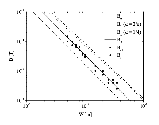
There are two data points in Fig. 3 for each strip width: The upper point indicates the lowest induction at which vortices were observed trapped in the strip, and the lower point indicates the highest induction at which vortices were not observed. This provides an upper and lower bound for the actual critical induction. It was apparent from this log-log plot that the critical induction depended on strip width as a power law. The best chi-square fit of the experimental data to the two parameter power law yielded and , taking a doubling of the best-fit chi-square as the uncertainty criterion. If we set the exponent to be (), a one parameter fit yielded . This is to be compared with for the present model [Eq. (9)], plotted as in Fig. 3. It should be emphasized that there were no fitting parameters in plotting .
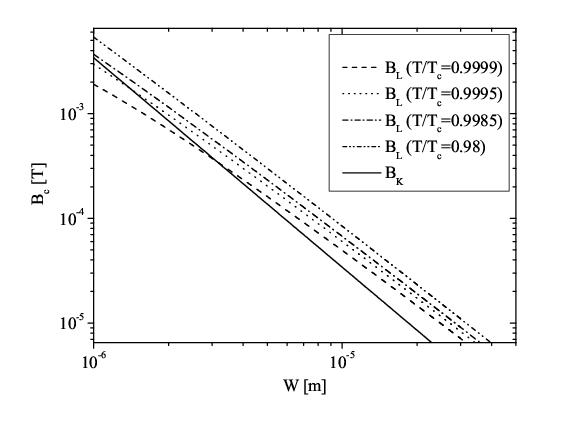
Comparison of the experiment with the models of Eqs. (5) and (9) is straightforward, since they are only dependent on the strip width. In order to evaluate Eq. (4) one must make an estimate of the temperature at which vortex freezout occurs because of the temperature dependence of . The depinning temperature used in Fig. 3 for both curves was calculated by Maurer et al.[20] for YBCO. In addition we used nm, a critical temperature of Tc = 93 K, and the two-fluid expression for the temperature dependence of the coherence length, resulting in nm. To the best of our knowledge the depinning temperature of YBCO has never been determined experimentally. Analysis of Eq. 4 shows that a closer to could give better agreement between theory and experiment for some strip widths. However the difference in slopes between theory and experiment becomes larger for higher , making it appear unlikely that this is the correct model for our results. The dependence of the Likharev model predictions on is displayed in Fig. 4 for . For lower ratios the curve moves further away from experiment.
We also compare results of the present model with previous work on Nb strips by Stan et al. [10] using SHPM. This paper reported critical inductions for 3 different strip widths: 1.6, 10 and 100 m. The critical inductions have been compared to the various models in Fig. 5. The depinning temperature of used in this figure was experimentally determined.[10] Using nm results in the value nm used for the curves in Fig. 5. A reasonably good agreement exists between the measurements and the predictions of the present model.

III.2 Trapped vortex density as a function of applied induction
In Fig. 6 the experimentally determined density of trapped vortices as a function of induction for two strip widths is displayed. This density depends nearly linearly on the difference between the induction and the critical induction, with a slope nearly , in agreement with previous work on Nb strips by Stan et al.[10]

The 35 m strip width data can be fit to a linear dependence of the vortex density on with a slope of Tm, with an intercept of T. The dashed and solid lines in Fig. 6 are the prediction of the present model [Eqs. (11) and (16) respectively] without any fitting parameters. Reasonable agreement exists between the present model and measurements. In the case of the 6 strips, there is an apparent saturation in the vortex density for inductions higher than 130 T. This may, however be an artifact due to the finite resolution of our SQUID sensor. The direction of the applied induction was reversed for three points in the m strip data to check for an offset in the applied induction. Such an offset, if present, was small, as indicated by the symmetry of the data around zero induction.
III.3 Vortex spatial distribution
The local minimum in the Gibbs free energy at of Eq. (3) makes it energetically favorable for vortices to be trapped in the center of the strip. However, as the vortex density increases, the vortex-vortex repulsive interaction makes it energetically more favorable to form an Abrikosov-like triangular pattern. Simulations on the trapped vortex position in strips was described by Bronson et al.[12] In particular they predict that there should be a single line of vortices for inductions . Above this induction range a second line of vortices is predicted to form. As the induction is increased further additional lines of vortices are predicted to form into a nearly triangular lattice.

We have investigated the distribution of vortices trapped in our strips at various inductions. As can be seen from the images of Fig. 2, even though there was significant disorder in the vortex trapping positions, there was also some apparent correlation between the vortex positions. An example can be seen in Fig. 7, where a histogram is displayed of the lateral positions of vortices trapped in the 35 m wide strip for several inductions. At low inductions, the vortex lateral position distribution peaked near the center of the film because the vortices were aligned nearly in a single row. At a second critical induction of T the distribution started to become broader. At 18 T there were two clear peaks in the distribution, corresponding to two rows. Using the value of T for the critical induction of the 35 m wide strips from our linear fit of the vortex density vs. applied induction curve of Fig. 6, we found . This is consistent with the prediction of of Bronson et al.[12] In the same paper the critical induction for the transition from the two-row to the three-row regime is given to be . This gives T using the same value for . In our measurements we saw no evidence for a three row regime. It was not possible to perform analysis at higher fields than reported here because of limitations to the spatial resolution of the SSM.

We also saw evidence for longitudinal ordering. In Fig. 8a-c histograms are displayed of the longitudinal distances between vortices in the 35 m wide strip for various inductions. As expected the inter-vortex spacing distributions became narrower as the inductions increased, since the vortex mean spacings decreased. However the distributions became narrow faster than their means as the induction was increased, indicative of longitudinal ordering, until the second critical induction of approximately 10 T was reached. At that induction the relative distribution width has a discontinuous jump as a second row starts to form. A similar decrease in the relative longitudinal distribution width with increasing induction is observed in the 6 m wide strip, although the spatial resolution of the SSM was not sufficient to resolve vortices at the second critical induction for this width.
In theory there should be longitudinal ordering independent of the magnetic induction. After all, the Gibbs free energy is independent of the position along the strip and the only interaction that plays a role is the interaction between the vortices. Differences in longitudinal ordering as a function of the magnetic induction could arise from local minima of the Gibbs free energy caused for example by defects in the material. For relatively low inductions vortices can easily be trapped in defects since the interaction between the vortices is small because the separation between the vortices is large. For higher magnetic inductions the number of vortices and likewise the interaction between the vortices increases. This could mean that the vortices are more likely to trap at positions determined by the minimization of the vortex-vortex energy than at positions determined by local defects.
IV Conclusions
Experiments on vortex trapping in narrow YBCO strips using a scanning SQUID microscope, as well as previous measurements on Nb,[10] showed a critical induction for the onset of trapping and a dependence of the vortex density on the induction which were in good agreement with a new model which takes into account the energy required to generate a vortex-antivortex pair. In addition, at low inductions the vortices formed a single row, with longitudinal ordering as the inductions increased. Formation of a second row was observed at a second critical induction consistent with numerical modeling.
V Acknowledgments
This research was financed by the Dutch MicroNED program and a VIDI grant (H.H) from the Dutch NWO Foundation. J.R.K was supported by the Center for Probing the Nanoscale, an NSF NSEC, NSF Grant No. PHY-0425897, and by the Dutch NWO Foundation. J.R.C’s work at the Ames Laboratory was supported by the Department of Energy-Basic Energy Sciences under Contract No. DE-AC02-07CH11358. The SSM setup used in this research was donated to the University of Twente by the IBM T.J. Watson Research Center.
References
- [1] M. Tinkham, Introduction to Superconductivity, 2nd Edition (McGraw-Hill, New York, 1996).
- [2] E. Dantsker, S. Tanaka, and J. Clarke, Appl. Phys. Lett. 70, 2037 (1997).
- [3] F. Schmidt, S. Linzen, F. Schmidl, M. Mans, and P. Seidel, Supercond. Sci. Technol. 15, 488 (2002).
- [4] A. Chwala, R. IJsselsteijn, T. May, N. Oukhanski, T. Schuler, V. Schultze, R. Stolz, and H. Meyer, IEEE Trans. Appl. Supercond. 13, 767 (2003).
- [5] S. Lee, W. Myers, H. Grossman, H.-M. Cho, Y. Chemla, and J. Clarke, Appl. Phys. Lett. 81, 3094 (2002).
- [6] A. Jansman, M. Izquierdo, J. Flokstra, and H. Rogalla, IEEE Trans. Appl. Supercond. 9, 3290 (1999).
- [7] J. Clem, Bull. Am. Phys. Soc. 43, 401 (1998), paper K36.06, and unpublished work.
- [8] K. Likharev, Sov. Radiophys 14, 722 (1972).
- [9] E. Dantsker, S. Tanaka, P.-A. Nilsson, R. Kleiner, and J. Clarke, Appl. Phys. Lett. 69, 4099 (1996).
- [10] G. Stan, S. Field, and J. Martinis, Phys. Rev. Lett. 92, 097003 (2004).
- [11] J. Kirtley, M. Ketchen, C. Tsuei, J. Sun, W. Gallagher, L. S. Yu-Jahnes, A. Gupta, K. Stawiasz, and S. Wind, IBM Journal of Research and Development 39, 655 (1995).
- [12] E. Bronson, M. Gelfand, and S. Field, Phys. Rev. B 73, 144501 (2006).
- [13] M. Tinkham, Phys. Rev 129, 2413 (1963).
- [14] V. Kogan, Phys. Rev. B 49, 15874 (1994), ISSN 0163-1829.
- [15] G. Maksimova, Phys. Solid State 40, 1607 (1998), ISSN 1063-7834.
- [16] A. A. B. Brojeny, Y. Mawatari, M. Benkraouda, and J. R. Clem, Supercond. Sci. Technol. 15, 1454 (2002).
- [17] M. Benkraouda and J. R. Clem, Phys. Rev. B 53, 5716 (1996).
- [18] M. Benkraouda and J. R. Clem, Phys. Rev. B 58, 15103 (1998).
- [19] V. Kogan, Phys. Rev. B 75, 64514 (2007), ISSN 1098-0121.
- [20] S. Maurer, N.-C. Yeh, and T. Tombrello, Phys. Rev. B 54, 15372 (1996).