The Effect of Pion Exchange
in a Relativistic Quark Model of Baryons

The radial wave functions $\psi_{a,b}$ in Eq. (2) were obtained by solving the Dirac equation for massless quarks in a linear scalar potential of the form [3, 15]

where the negative offset, $-\kappa^{2}r_{0}$, effectively gives these massless quarks a constituent mass. (It also affords inclusion of a rough representation of the effect of the short-distance color Coulomb interaction between quarks.) For the values used in Goldman, Maltman, Stephenson and Schmidt [3] (referred to henceforth as GMSS), $\kappa^{2}=0.9$ GeV/fm and $r_{0}=0.57$ fm, the bound quark has a total energy of 361.6 MeV . The upper and lower radial wave functions, $\psi_{a}(r)$ and $\psi_{b}(r)$, are chosen real in this description.

The radial functions $\psi_{a,b}(r)$ were found in GMSS by numerically solving the Dirac equation with the linear scalar potential of Eq. (3). In this form, they have dimensions ${\rm fm}^{-3/2}$ and are normalized so that

Following Critchfield [15], we can express the $\psi_{a,b}(r)$ in terms of dimensionless, unnormalized functions $\phi_{a,b}(\kappa r)$, where $\kappa=2.1357$ ${\rm fm}^{-1}$ (the GMSS value), as

Explicitly separating out the natural scale of the problem, $\kappa$, allows us to define the normalization factor, $N$, to be dimensionless also.

The numerical solutions for $\phi_{a,b}(x)$, $x=\kappa r$, have been well fitted (in GMSS’s Appendix B) as a sum of Gaussians,

where we have defined $\tilde{\mu}_{k}=\mu_{k}+1$. The (dimensionless) coefficients $a_{k}$, $b_{k}$, and $\mu_{k}$ are tabulated in Appendix B of GMSS for $n=6$, 12, and 18 Gaussian terms. For our purposes, the table for six terms provides sufficient accuracy. With Eqs. (6) and (7) for $\phi_{a,b}$, we can calculate the normalization constant, finding

Let us now calculate the interaction energy $B^{(1,2)}_{qq\pi}(r_{\rm cut})$ between these two quarks. With Eq. (2), the two wave-function factors we need are

Thus,

where

Here $\mu=m_{\pi}/\kappa$, ${\bf x}_{1}=\kappa{\bf r}_{1}$, ${\bf x}_{2}=\kappa{\bf r}_{2}$, $x=|{\bf x}_{1}-{\bf x}_{2}|$, and $x_{\rm cut}=\kappa r_{\rm cut}$.

Since all vectors in Eq. (12) are integrated out, the tensor $I_{\alpha\beta}$ reduces to

where

Physically, this simplification happens because the pion-exchange interaction between two spin-$\frac{1}{2}$ particles in a relative $S$-wave can only involve the central scalar, but not the tensor, contribution.

To evaluate the integral of Eq. (14), we will do the ${\bf x}_{2}$ integration first, rewriting

where

To proceed, let the integration variable for $J({\bf x}_{1},x_{\rm cut})$ be ${\bf x}={\bf x}_{1}-{\bf x}_{2}$, with $x$ running from $x_{\rm cut}$ to $\infty$. As Eq. (16) has no vectorial dependence remaining after the integrations,

with $\cos\theta={\bf\hat{x}}_{1}\cdot{\bf\hat{x}}$. Defining

and using Eqs. (6) and (7),

The factor of $|{\bf x}_{1}-{\bf x}|$ here cancels the denominator in Eq. (17). Expanding $|{\bf x}_{1}-{\bf x}|^{2}$ as $x_{1}^{2}+x^{2}-2x_{1}x\cos\theta$, we can write

where

The double integral in Eq. (21) can be done analytically, yielding

where

and

(For definitions of the error functions, see Ref. [16].) In the equation for $B_{k_{1}k_{2}}$ we have defined

One might worry that the integration over $x_{1}$ that follows in Eq. (15) would blow up because of the $e^{+\mu x_{1}}$ in the second term of $B_{k_{1}k_{2}}$. However, this exponential growth will be damped by the Gaussians in the $\phi_{a}(x_{1})\phi_{b}(x_{1})$ factor.

We have at this point reduced the six-fold integration in Eq. (11) to 36 simple, compact integrations over $x_{1}$, which we can easily (and quickly) evaluate numerically.

where

We have done the numerical integrations using Mathematica [17], which has a built-in ${\rm erfc}(x)$ function. For $r_{\rm cut}=1.0$ fm, for example, $\;I=-0.487$ MeV. The dependence of $\;I(r_{\rm cut})$ on $r_{\rm cut}$ is displayed in Fig. 1. Note that this function is repulsive for $r_{\rm cut}<0.6$ fm and attractive after that. This can be understood as due to the interplay between the cosine from ${\bf\hat{r}}_{1}\cdot{\bf\hat{r}}_{2}$ and the cutoff function $\Theta(r-r_{\rm cut})$. When $r_{\rm cut}$ is small, the angle between ${\bf\hat{r}}_{1}$ and ${\bf\hat{r}}_{2}$ can also be small enough so the cosine is positive. This combined with the resulting smaller $r$ means that the positive pion propagator factor can give larger contributions to the integrand. However, when $r_{\rm cut}$ gets sufficiently large, the two vectors will tend to contribute when they point in opposite directions. This makes the cosine negative, which makes the integrand negative for $r_{\rm cut}>0.6$ fm, even though the pion propagator factor is diminished in size.

As a check on our algebra, we have also calculated the triple integral in Eq. (15) for a few cases of $r_{\rm cut}$ numerically. This takes, of course, considerably more computing time and the calculation is slow to converge. However, the numerical results are in good agreement with the results shown in Fig. 1.

Altogether, contribution to the nucleon or $\Delta$ mass from the interaction energy of cut-off pion exchange between quarks 1 and 2 is

with the spin-isospin factor

Summing up over all pairs of the three quarks, the total $\pi$-exchange interaction energy contribution, after taking into account the coupling of the quark spins and isospins to total $S$ and $T$, is

where

The spin-isospin sum $X_{ST}$ can be evaluated in several ways. The most direct (most simplistic) is to write the operators $\mbox{\boldmath$\tau$}_{i}\cdot\mbox{\boldmath$\tau$}_{j}$ and $\mbox{\boldmath$\sigma$}_{i}\cdot\mbox{\boldmath$\sigma$}_{j}$ in terms of their raising, lowering, and the $z$-components. Then apply these expanded operators, in turn, for each combination of $i<j$ on the three-quark wave functions for the nucleon and $\Delta$. This proceeds quickly for the $\Delta$ state of highest weight, $|\Delta^{++},+3/2>$, and gives, after summing, the value 3. For the proton with spin-up, $|p,+1/2>$, however, it is a rather tedious calculation which eventually yields the value 15.

A more group-theoretic way of arriving at these numbers is given in an Appendix. However, a simple, heuristic derivation of $X_{ST}$ goes as follows. First note that, for any pair of quarks,

which is equal to $+1$ when the two quarks are in a triplet state and $-3$ when in a singlet. Likewise, $\mbox{\boldmath$\tau$}_{i}\cdot\mbox{\boldmath$\tau$}_{j}$ is $+1$ and $-3$ in iso-triplet and iso-singlet states. As mentioned earlier, each $S$-wave quark pair must be symmetric in the spin-isospin space.

For the $\Delta$, therefore, to get the total spin and isospin to both be $3/2$, each quark pair must have $S=T=1$. Thus

and summing over the three pairs then yields 3 for the value of $\Delta$’s $X_{ST}$.

For the nucleon, however, each quark pair can be in either an $S=T=1$ or an $S=T=0$ state, and it is equally likely to be one or the other. Thus

Now summing over the three pairs yields 15 for the value of nucleon’s $X_{ST}$.

Note that, between two quarks, the spin-isospin factor is either +1 ($S=T=1$) or +9 ($S=T=0$). Thus, for $r_{\rm cut}>$ 0.7 fm (see Fig. 1), Eq. (30) shows that the net interaction energy, $B_{qq\pi}^{(1,2)}$, is positive. This result is to be contrasted with the case of two nucleons in an $S$-wave. In that case there is no color quantum number to provide for antisymmetrization. Thus antisymmetry of the two fermions involved requires that $S=0$ and $T=1$ or $S=1$ and $T=0$ (deuteron), and hence the interaction energy from the pion exchange has the opposite sign: $(-3)\times(+1)=(+1)\times(-3)=-3$. Thus, while this pion-exchange interaction is attractive in both the deuteron and threshold state, it is repulsive between quarks in both the nucleon and the $\Delta$-baryon, as one expects for a self-energy contribution to a stable particle.

Since $X_{ST}$ is positive for both nucleons and $\Delta$’s, the total $B_{qq\pi}^{\rm tot}$ will also be positive for values of $r_{\rm cut}$ greater than 0.7 fm. That is, pion exchange between quarks produces a repulsive force within these baryons.

To evaluate this contribution to the baryon energy, we must fix the value of $g_{qq\pi}$, as noted after Eq.(1). To do this, we refer to results from the extended QDCSM [10] and some general features relating the chiral coupling of pions to the axial current, $f$, to the coupling, $g$, for the nominally equivalent (at low energies) pseudoscalar form (used here for its relative calculational simplicity). The usual relation at the nucleon level is

where the value of $f_{NN\pi}^{2}/(4\pi)=0.075$, as extracted from fits to nucleon-nucleon scattering [18, 14]. The factor of $2M_{N}$ compensates for the fact that in the pseudoscalar coupling, $\bar{\psi}\gamma_{5}\psi$, the upper and lower components of the Dirac wave function are coupled, with the lower being reduced, in momentum space, by a factor of order $m_{\pi}/(E_{N}+M_{N})\sim m_{\pi}/(2M_{N})$. The momentum scale is set by $m_{\pi}$ and the kinetic energy of the nucleon is small.

In the extended QDCSM [10], (which, as we noted previously, is a non-relativistic quark model of nucleon structure and nucleon-nucleon interactions extended from the QDCSM by the addition of pion exchange between quarks separated by a minimum distance), the relation between $f_{NN\pi}$ and $f_{qq\pi}$ is modified from the simple group-theoretic factor (5/3) by a small correction due to the quark delocalization within the nucleon, which accounts for the nucleon not being a point-like field lacking internal structure, viz.,

Here $b\approx 0.6$ fm describes the width of a single quark wave function in the nucleon and so provides for the experimentally determined root-mean-square size of the overall matter distribution in the nucleon. Since $m_{\pi}b\approx 0.4$, this correction is of order 10%, so that

Nonetheless, this value is not appropriate to our relativistic description here, as it has been extracted for non-relativistic wave functions. The effect is similar to the one evidenced in the right-hand-side of Eq.(34), as our lower wave function components are suppressed relative to the upper components by a factor of order $m_{\pi}/(E_{q}+m_{q})$, the relevant ratio corresponding to what we saw above for the nucleon. Since the quarks here are highly relativistic, but with an energy of order one-third of the mass of the nucleon, the suppression is therefore not as great as for the case of the very non-relativistic nucleon. Since this suppression is already present in the scale of our lower wave function components, it follows that the appropriate value to use is

where we have taken $E_{q}=361.6$ MeV and $m_{q}\simeq 0$, as in the LARQ. Note that this is approximately two orders-of-magnitude smaller than the value for nucleons, $g_{NN\pi}^{2}/4\pi$, which suggests a more valid perturbation theory.

The function $I(r_{\rm cut})$ reaches its minimum near $r_{\rm cut}=1.05$ fm, where its value is $-0.492$ MeV. Multiplying together the various factors in Eq. (30), the maximum contribution for this exchange energy is

This contribution to the self-energy produces a small change in mass, compared to rest masses of these baryons. It is comparable to electromagnetic corrections, which have been ignored at this level.

This allows us to conclude that the fitted parameters of the LARQ model for the nucleon and $\Delta$ baryons are not significantly affected by inclusion of this pion-exchange contribution between the quarks. The only remaining concerns are related to quark self-energy corrections, which we will deal with in following section.

For larger values of $r_{\rm cut}$, such as the 1.4 fm cutoff advocated in Ref. [14], this contribution is even smaller. It is also interesting that, for a value of $r_{\rm cut}\approx$ 0.7 fm (as suggested by the MIT bag model [19]), this contribution is exceptionally small, since $I(r_{\rm cut})$ crosses the $x$-axis near that value.

However, none of this implies that the predictions of the LARQ model for nuclei, such as the deuteron, will be unchanged by this pion-exchange contribution. There, significant cancellations affect the net value of the binding energy. Hence it is still necessary to extend these calculations to the nuclear cases, and to determine the change in this pion-exchange interaction energy as the quark wave function changes in each particular nucleus.

We begin by evaluating the first approximation to the loop correction. For a quark labeled “1” and a quark in the intermediate state labeled “2”,

where $<\mbox{\boldmath$\tau$}\cdot\mbox{\boldmath$\tau$}>=3$ and

Again, the $\Theta$-function assures that $r=|{\bf r}_{1}-{\bf r}_{2}|\geq r_{\rm cut}$ . For the $S$-wave quark wave functions of Eq. (2) we find

and

Multiplying Eqs. (41) and (42) and using completeness of the spin function, $\sum_{s_{2}}\chi_{s_{2}}\chi_{s_{2}}^{\dagger}=1$, we find

where we have made use of the reality of the wave functions, the anticommutator $\{\sigma_{\alpha},\sigma_{\beta}\}=\delta_{\alpha\beta}$, and the interchange symmetry/equivalence of $r_{1}$ and $r_{2}$ to combine terms.

With the pion Green’s function factor, $e^{-m_{\pi}r}/r$, the integral over the first term in Eq. (43) is two times $I(r_{\rm cut})$, which we defined in the previous section and calculated to have the form given in Eqs. (14) and (26). Thus, the self energy for a single quark from a pion loop consists of two terms,

The new contribution to $B_{qq\pi}^{SE}$, $\widetilde{I}(r_{\rm cut})$, comes from the last term in Eq. (43). For a three-quark baryon, the total self-energy correction from pion loops will be three times $B_{qq\pi}^{SE}$.

We can evaluate $\widetilde{I}$ in a way very similar to that for the more complicated $I$.

where

Note that $\widetilde{I}$ is positive and there will be some cancellation in Eq. (44) with $I$, which is negative for values of $r_{\rm cut}$ of interest. How much cancellation depends on the relative sizes of $I$ and $\widetilde{I}$.

Proceeding as in the previous section, with the Gaussian expansion of $\phi_{a}(x)$ defined in Eqs. (5-8), we find, after some algebra,

The quantities $c_{k_{1}k_{2}}$ and $t_{k_{1}k_{2}}^{(\pm)}(x_{\rm cut})$ are the same as above, defined before Eq. (19) and in Eq. (25). Inserting $\widetilde{J}$ in Eq. (45), we have finally

where

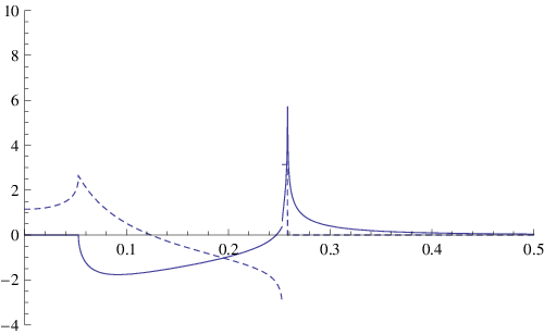
We have again evaluated this sum of one-dimensional integrals using Mathematica. It is a monotonically falling function ranging from 11.88 MeV at $r_{\rm cut}=0.6$ fm to 0.275 MeV at $r_{\rm cut}=1.8$ fm. For $r_{\rm cut}=1.0$ fm, $\widetilde{I}$ = 6.17 MeV, quite a bit larger than $I$ at this value of $r_{\rm cut}$ (-0.487 MeV). Thus the sum of the integrals in the square bracket in Eq. (44) is dominated by the $\widetilde{I}$ term. The solid curve in Fig. 3 shows the dependence of $B_{qq\pi}^{SE}$ on $r_{\rm cut}$. (The dashed curve shows the dominant contribution due to $\widetilde{I}(r_{\rm cut})$.)

For $r_{\rm cut}=1.4$ fm that square bracket has a value of 1.436 MeV and the total value of the quark self-energy loops is $B_{qq\pi}^{{\rm tot,}\;SE}$ is 4.39 MeV. This is the contribution of all three quarks in a nucleon (or $\Delta$) for this value of $r_{\rm cut}$. In comparison, for the nucleon, the exchange energy from pion exchange between the three quarks at the same value of $r_{\rm cut}$ is, from Eq. (30), 2.58 MeV. If this value were not much changed by the inclusion of higher energy intermediate states, it would be clear that the LARQ parameters are not significantly affected by the addition of “long-distance” pion exchanges. We next test this conclusion by using a free propagator approximation for the intermediate state.

To compare with the above approximation we now evaluate, in four-momentum space, the pion-loop self-energy correction using a free-quark propagator in the intermediate state. This energy is, for a bound quark with four-momentum $p_{\mu}=(E,|{\bf p}|)$, $E=0.362$ GeV, an intermediate pion with four-momentum $k_{\mu}$, and a massless intermediate free quark with four-momentum $(p-k)_{\nu}$,

The factor of 3 comes from the isospin factor, $<\mbox{\boldmath$\tau$}\cdot\mbox{\boldmath$\tau$}>$.

The loop integral $J_{\nu}$ defined in Eq. (50) is

since $p_{\nu}$ is the only available four-vector for defining the $\nu$-component. Its coefficient is

which will be evaluated below.

With $\bar{\psi}_{s}(p)=\psi_{s}^{\dagger}(p)\gamma_{0}$ and the factor of $p_{\nu}$ from $J_{\nu}$, the Dirac matrices in Eq. (50) reduce to

References

- [1] T. Goldman, K. Maltman, G. J. Stephenson, Jr., Jia-Lun Ping, and Fan Wang, Mod. Phys. Lett. A13, 59 (1998).
- [2] T. Goldman, K. Maltman and G. J. Stephenson, Jr., Phys. Lett. B324, 1 (1994).
- [3] T. Goldman, K. R. Maltman, G. J. Stephenson, Jr., and K. E. Schmidt, Nucl. Phys. A481, 621 (1988). This reference is henceforth abbreviated as GMSS.
- [4] J. J. Aubert et al. Phys. Lett. B123, 275 (1983). For a comprehensive review, see D. F. Geesaman, K. Saito, and A. W. Thomas, Ann. Rev. Nucl. Part. Sci. 45, 337 (1995).
- [5] C. J. Benesh, T. Goldman, and G. J. Stephenson, Jr., Phys. Rev. C 68, 045208 (2003).
- [6] M. Hirai, S. Kumano and M. Miyama, Phys. Rev. D 64, 034003 (2001); M. Hirai, S. Kumano, T.-H. Nagai, arXiv: 0709.3038.
- [7] Fan Wang, Guang-han Wu, Li-jian Teng and T. Goldman, Phys. Rev. Lett. 69, 2901 (1992), Chin. Sci. Bull. 38, 1257 (1993) [nucl-th/9210002]. See also, G. Wu, J. Ping, L. Teng, F. Wang and T. Goldman, Nucl. Phys. A 673, 279 (2000) [nucl-th/9812079].
- [8] J. Ping, F. Wang and T. Goldman, Nucl. Phys. A 657, 95 (1999) [nucl-th/9812068].
- [9] Xi-Feng Lu, Jia-Lun Ping and Fan Wang, Chin. Phys. Lett. 20, 42 (2003) [nucl-th/0702035].
- [10] J. Ping, F. Wang and T. Goldman, Phys. Rev. C 65, 044003 (2002) [nucl-th/0012011].
- [11] H. A. Bethe, Phys. Rev. 57, 260 and 390 (1940).
- [12] T. Inoue, V. E. Lyubovitskij, Th. Gutsche, and A. Faessler, Int. J. Mod. Phys. E15, 121 (2006).
- [13] See, e.g., J. L. Friar, B. F. Gibson, and G. L. Payne, Phys. Rev. C 30, 1084 (1984).
- [14] See, e.g., M. M. C. Rentmeester, R. G. E. Timmermans, J. L. Friar and J. J. de Swart,Phys. Rev. Lett. 82, 4992 (1999); M. M. C. Rentmeester, R. G. E. Timmermans and J. J. de Swart, Phys. Rev. C 67, 044001 (2003).
- [15] For the case when , see C. L. Critchfield, Phys. Rev. D 12, 923 (1975).
- [16] See, e.g., M. Abramowitz and I. A. Stegun, Handbook of Mathematical Functions, (National Bureau of Standards, reprinted 1968 by Dover Publications, New York), Chapter 7.
- [17] Mathematica is a product of Wolfram Research, and its use is described, for example, by S. Wolfram in The Mathematica Book, 4th ed. (Cambridge University Press, Cambridge, 1999)
- [18] J. L. Friar, private communication.
- [19] T. DeGrand, R. L. Jaffe, K. Johnson, and J. Kiskis, Phys. Rev. D 12, 2060 (1975).
- [20] P. J. A. Bicudo, G. Krein and J. E. F. T. Ribiero, Phys. Rev. C 64, 025202 (2001) [hep-ph/0105289].
- [21] M. Ottel and A. W. Thomas, Phys. Rev. C 66, 065207 (2002) [nucl-th/0203073].
- [22] P. Isacker, O. Juillet and B. K. Gjelsten, Foundations of Physics 27, 1047 (1997).
- [23] J. N. Ginocchio, private communication.