Dyson–Maleev representation of nonlinear sigma-models
Abstract
For nonlinear sigma-models in the unitary symmetry class, the non-linear target space can be parameterized with cubic polynomials. This choice of coordinates has been known previously as the Dyson-Maleev parameterization for spin systems, and we show that it can be applied to a wide range of sigma-models. The practical use of this parameterization includes simplification of diagrammatic calculations (in perturbative methods) and of algebraic manipulations (in non-perturbative approaches). We illustrate the use and specific issues of the Dyson-Maleev parameterization with three examples: the Keldysh sigma-model for time-dependent random Hamiltonians, the supersymmetric sigma-model for random matrices, and the supersymmetric transfer-matrix technique for quasi-one-dimensional disordered wires. We demonstrate that nonlinear sigma-models of unitary-like symmetry classes C and B/D also admit the Dyson-Maleev parameterization.
I Introduction
I.1 Nonlinear sigma-models
Extensive studies of disordered systems in last decades have identified the nonlinear sigma-model (NLSM) formalism as a universal tool for describing the low-energy properties of such systems [1, 2, 3, 4, 5, 6, 7, 8, 9]. The underlying idea of the NLSM approach is that the low-energy physics of disordered systems is determined by soft collective excitations (usually referred to as diffusons and cooperons). Therefore one can integrate out the high-energy degrees of freedom and end up with an effective theory which contains only soft collective modes. The resulting theory is a NLSM, which is a field theory formulated in terms of a matrix field subject to a nonlinear constraint . Depending on the way of handling disorder averaging, the -matrix can act either in the supersymmetric [2, 3, 4, 5], replica [6, 7] or Keldysh [8, 9] spaces. Besides that, the -field can be a function of continuous space and/or time coordinates, and also have an additional matrix structure due to an additional symmetry of the initial Hamiltonian.
The NLSM action usually has a hydrodynamic form, containing only the lowest powers of , e.g.,
| (1) |
where implies the full trace, involving integration over continuous coordinates (in the supersymmetric formalism, the trace over the superspace is the supertrace). The action (1) determines the weight in the functional integral which should be performed over the manifold
| (2) |
where
| (3) |
in the “retarded-advanced” space, and span an appropriate group of rotations. The matrices (or operators) and in (1) must commute with : , so that is a saddle point of the action.
Depending on the symmetries of the disordered problem, the initial Hamiltonian may have additional symmetries, which translate into additional linear constraints on the matrix (realized in terms of extending its dimension, in combination with imposing constraints on the rotations ) [4, 10].
The NLSM is a complicated field theory, and its exact solution is possible only in a few exceptional cases: zero-dimensional supersymmetric sigma-model for level statistics of random matrices[2, 4], and one-dimensional supersymmetric sigma-model for quasi-one-dimensional localization[11, 4, 5]. In a situation where the integration over the whole manifold of matrices cannot be performed exactly, the sigma-model can be treated with the standard perturbative approach, applicable in the weak-coupling limit (large conductance). Solution of the NLSM in the strong-coupling limit (small conductance) is a challenging and so far unresolved task.
In the weak-coupling limit, a widely used perturbative expansion of the NLSM around the saddle point is based on the parameterization of the curved -matrix manifold in terms of an unconstrained matrix :
| (4) |
where can be an arbitrary function satisfying . A particular choice of the function is a matter of convenience (see discussion of various parameterizations in Ref. 12), and the calculated correlation functions do not depend on it. The integration contour in the space of and should be chosen consistently with the convergence of the integrals performed in the derivation of the NLSM. In the supersymmetric formalism, this amounts to the requirement of the compact fermionic and non-compact bosonic sectors[2, 3].
If the action (1) possesses several saddle points, an analogous perturbative expansion should be carried out around each of them.
Substituting expressed in terms of into the initial action (1), one arrives at a new theory
| (5) |
with the action and, generally speaking, with a Jacobian . This new theory can be treated with the help of the standard perturbative approach by separating the action into the Gaussian part, , and the rest taken into account perturbatively. However, the initial action (1), which was a finite polynomial in terms of , typically becomes an infinite series in terms of . This makes higher-order perturbative calculations very involved as one has to take into account a rapidly growing number of diagrams made of various higher-order vertices .
I.2 Dyson–Maleev parameterization
For nonlinear sigma-models in the unitary symmetry class, there exists a remarkable parameterization which does not belong to the infinite-series family (4). The non-linear target space can be parameterized by cubic polynomials:
| (6) |
The asymmetry between the and matrices is the price one has to pay for finite number of terms in the parameterization (6). It can be shown by a direct calculation that the Jacobian of this transformation is unity, and thus the integration measure over and is flat: . In the new variables, the NLSM action becomes a finite-order polynomial, e.g., the action (1) becomes a sum of the bilinear and quartic in , terms:
| (7) |
The absence of higher-order interaction vertices greatly reduces the number of diagrams in the perturbative expansion, which considerably simplifies routine calculations.
The parameterization (6) is closely related to the famous Dyson-Maleev [13, 14] (DM) parameterization for quantum spins. In that representation, the spin- operators are expressed by the boson creation and annihilation operators and as
| (8) |
The Dyson-Maleev parameterization produces the correct spin commutation relations but violates the property , and thus renders the spin Hamiltonian manifestly non-Hermitian. An alternative approach based on the Holstein-Primakoff parameterization [15] [which is in fact a counterpart of the parameterization (4) with ] respects Hermiticity but generates an infinite series of interaction vertices. The Dyson–Maleev transformation has proven to be the most convenient tool for studying spin-wave interaction in ferromagnets [16, 17]: it reproduces all the perturbative results obtained with the Holstein-Primakoff parameterization in a much faster and compact way. Owing to the analogy with the Dyson–Maleev representation of spin operators, the transformation (6) will be referred as the Dyson–Maleev representation of the NLSM.
In the original DM representation for spin operators, the Hilbert space of free bosons should be truncated in order for the operator to have a bounded spectrum. This truncation of the bosonic Hilbert space is irrelevant for perturbative calculation but becomes essential in the non-perturbative regime when the expectation value is comparable to . Clearly, some analogy of this Hilbert space truncation should be present also in the functional NLSM language. Indeed, in this paper we demonstrate that imposing certain conditions on the eigenvalues of the matrix makes the DM representation non-perturbatively equivalent to the original NLSM in terms of the field.
At the perturbative level, the DM transformation (6) has been applied for the analysis of the replicated[18] and Keldysh[12] sigma-models (cf. also the usage of the DM transformation [19] for two-dimensional classical ferromagnets). At this level, when fluctuations are small, it suffices to use formally the parameterization (6) without taking care of the exact integration region over and . We illustrate the details of the perturbation theory in the DM parameterization with the examples of the Keldysh sigma-model for time-dependent random Hamiltonians in Sec. II.
At the non-perturbative level, the DM transformation (6) can be considered as an alternative parameterization of the complex manifold . Therefore, changing variables from to and may be considered as a contour deformation on the NLSM manifold which leaves the functional integral invariant. We do not give a rigorous proof of this statement but demonstrate the non-perturbative exactness of the DM transformation on the example of the supersymmetric NLSM for unitary random matrices in Sec. III.
Another advantage of the DM representation is that it provides a compact algebraic way for deriving non-perturbative transfer-matrix equations for the one-dimensional NLSM. We demonstrate this with the diffusive supersymmetric sigma-model for quasi-one-dimensional localization [2] where the use of the DM transformation allows to derive the transfer-matrix Hamiltonian “without fermions”, using just the algebraic properties of the corresponding symmetric space, see Sec. IV.
Finally, in Sec. V we show that the DM transformation introduced for the unitary symmetry class can be extended to other unitary-like symmetry classes C and B/D introduced by Altland and Zirnbauer[20] in the context of superconductivity.
The main facts about the Dyson-Maleev transformation are summarized in Sec. VI.
II Perturbation theory: Keldysh sigma-model for time-dependent random Hamiltonians
We illustrate the utility of the DM formalism in the perturbative regime with the problem of a quantum particle subject to a time-dependent random unitary Hamiltonian . This problem has been studied in the framework of the Keldysh sigma-model [12], and the use of the DM parameterization has been shown to greatly reduce the number of diagrams, in comparison with the usual infinite-series parameterization (4).
II.1 The model
In a semiclassical approximation, the dynamics of a particle subject to quantum evolution with a non-stationary Hamiltonian can be described as a diffusion process in the energy space. Diffusive spreading of the wave function is characterized by the diffusion coefficient which determines the rate of the energy drift with time :
| (9) |
with being the mean level spacing. The dimensionless diffusion coefficient depends on the rate of variation of the Hamiltonian measured by the dimensionless velocity of adiabatic energy levels:
| (10) |
In the limit , the energy absorption is due to transitions in the continuous spectrum, and this regime can be described by the linear-response Kubo formula [21, 22]. In the opposite limit, , energy is absorbed during rare Landau–Zener transitions between neighboring levels. In these limiting cases, the diffusion coefficient has been obtained by Wilkinson [21]:
| (11) |
where , and 4 for the orthogonal, unitary, and symplectic ensembles, respectively, and are numerical coefficients. Quite surprisingly, for the unitary ensemble, indicating that both in the limits of small and large .
Unfortunately, the methods used in Ref. 21 to get the asymptotics (11) cannot be generalized to finite values of . A general approach to calculating the full dependence based on the Keldysh sigma-model formalism has been derived in Ref. 23. The field variable is the operator which is the integral kernel in time domain with values in matrices in the Keldysh space (analogous to the retarded-advanced space in the supersymmetric formalism). The -matrix is subject to the constraint , where a convolution over time arguments is implied. As usual, the integration manifold is the orbit (2) of (Pauli matrix in the Keldysh space) under unitary rotations . In the dimensionless form (time measured in units of ), the Keldysh action for the linearly driven random unitary Hamiltonian takes the form [23, 12]
| (12) |
where the coupling parameter is defined in Eq. (10), and denotes the trace over the two-dimensional Keldysh space. The parameter plays the role of the dimensionless conductance which controls the strength of fluctuations around : they are small for and strong for .
The NLSM (12) contains full information about the function which can be expressed as [12]
| (13) |
where the diffuson is defined through the correlation function of the off-diagonal components of the field:
| (14) |
II.2 Dyson-Maleev transformation
The propagator of the quadratic part of the action (15) is given by
| (16) |
where is the bare diffuson:
| (17) |
Substituting (17) into (13), one gets the large- Kubo result . Treating the quartic term in the action (15) as a perturbation, we can compute the perturbative series for the diffuson and, consequently, for in the limit of large . From simple power counting [23], -loop diagrams give a contribution to proportional to . For the unitary ensemble, the number of loops must be even, which corresponds to expanding in powers of :
| (18) |
In two loops, it has been found that (the nullification of this diagram is nontrivial, and we are not aware of any symmetry reasons for this fact)[23, 24]. In the DM parameterization, there is just one two-loop diagram, while the standard infinite-series parameterization (4) generates two distinct diagrams, one made of a 6-order vertex, and another made of two 4-order vertices. While the DM parameterization appears to be the most compact way of getting the analytic expression in two loops, its use at this order of perturbation theory is not crucial.
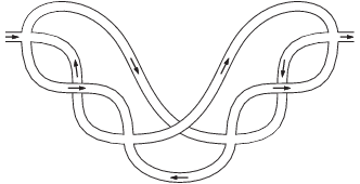
The coefficient is determined by four-loop diagrams. Its calculation performed in Ref. 12 was only possible with the use of the DM parameterization. Indeed, four-loop diagrams in an arbitrary infinite-series parameterization (4) would contain interaction vertices of the and fields up to the tenth order. Then even a classification of the four-loop diagrams becomes a sophisticated problem. On the other hand, in the DM formalism with the single quartic term in the action (15), there are only 20 irreducible four-loop diagrams for the diffuson self-energy, see an example in Fig. 1. Some of them are related by symmetries, and the total number of nonequivalent diagrams is 9. They are given by seven-fold time integrals of the form
where and are homogeneous polynomials of degrees six and three, respectively. Numerical evaluation of these integrals shows that is zero within the accuracy of the calculation and supplies the upper bound for its absolute value: . A further discussion of this result can be found in Ref. 12.
To conclude this Section, we mention that the same diagram classification applies to a wide class of NLSM with the action (1), whose Dyson-Maleev representation (7) contains only the Gaussian and quartic terms. In particular, quantum dynamics with an arbitrary time dependence of the Hamiltonian can be described by the Keldysh action (12) with the slightly modified last term[23, 25], thus also admitting the DM parameterization with the quartic interaction [12]. Finally, various versions of diffusive sigma-models also belong to this class and have the same diagram classification in the DM representation.
III Non-perturbative approach: supersymmetric NLSM for unitary random matrices
We start discussing the non-perturbative aspects of the DM transformation with the simplest example of the supersymmetric NLSM for the spectral statistics of unitary random matrices.
The theory is formulated in terms of the supermatrix acting in the direct product of the superspace (BF) and the retarded-advanced space (RA). The pair correlation function of the density of states, , is given by the integral [2, 4]
| (19) |
Here is the mean level spacing, , and is the supersymmetry-breaking matrix. The supertrace is defined as the bosonic trace minus fermionic trace. The sigma-model action is
| (20) |
With the non-compact BB sector and compact FF sector, the action (20) possesses two saddle points: the standard saddle point (“north pole of the fermionic sphere”) and (“south pole of the fermionic sphere”), both belonging to the same connected component. The “south pole” is known to be responsible for oscillations in the pair correlation function [26].
The DM transformation (6) may be considered as a special change of variables which parameterizes almost the whole complex manifold . However the “south pole” does not correspond to any finite and and can be achieved only as a limiting point for , at .
In Efetov’s parameterization [2, 4], the integration contour over is chosen in such a way that the eigenvalues and of the block are real and bounded to the strip
| (21) |
(the eigenvalues of the block are the opposite: and ). Now a transition from Efetov’s parameterization of the -manifold to the DM parameterization can be realized as a deformation of the integration contour in a multi-dimensional space. It will be convenient to impose an additional requirement that the eigenvalues of the block (and the block as well) do not change during the deformation. Since the eigenvalues of the product are given by and , this requirement constrains the eigenvalues of to be real and to belong to the corresponding strip. The constraint on the eigenvalues of is reminiscent of the truncation of the bosonic Hilbert space in the original DM transformation for spin operators (where it is formulated as the constraint on the eigenvalues of the number of bosons ). We may also note a similar restriction of the integration region in the theory of the DM parameterization for classical ferromagnets [19].
Throughout the deformation from Efetov’s to DM parameterization, we may maintain the unchanged relation between the commuting components of and :
| (22) |
This choice of the real section of the complex manifold respects the correct domains for and . The independent elements are the two complex numbers and , and the four Grassmann numbers , , , (we do not use complex conjugation of Grassmann variables in our formalism). An arbitrary integral over can then be rewritten in the DM variables as
| (23) |
where is the step function, and is the standard flat measure:
| (24) |
The integral (23) may be calculated straightforwardly in the variables using the explicit expression for the eigenvalues of the product :
| (25) | |||
| (26) |
These formulas allow a direct calculation of correlation functions in the DM parameterization.
III.1 Technicalities of the integration over and
We illustrate the above approach by calculating the integral
| (27) |
which for a suitable choice of the functions and gives the level-level correlation function (19).
Note that in the flat parameterization used, does not depend on Grassmann variables. A direct calculation (expanding in Grassmann variables) shows, quite surprisingly, that the same is true for two step functions in (27): , . Therefore, only two terms in the integrand (27) contain Grassmann variables: and . Expanding these functions in Grassmann variables and evaluating the integral over them, after a straightforward but lengthy calculation we arrive at
| (28) |
where the second term is the anomaly contribution. In particular, it is responsible for the proper normalization for .
To find the level-level correlator (19), we should use (28) with and . Evaluating the integrals over and we arrive at the well-known result [27]
| (29) |
By reproducing the standard expression (29) we demonstrate that restricting the integration region over and to the strip (21) makes the DM transformation non-perturbatively equivalent to the initial NLSM in the -representation.
To be precise, our example (27) involve only the diagonal blocks and . Therefore, our derivation is equivalent to that in the Hermitian “square-root-odd” parameterization [28, 12] of the type (4) with which has unit Jacobian. This parameterization has the same diagonal blocks as the DM one and the same integration measure.
In fact, a continuous interpolation is possible between the “square-root-odd” and DM parameterization, such that the diagonal blocks and remain unchanged, and the Jacobian equals one throughout the interpolation[29].
The power of the DM parameterization will come in the full glory in the next Section when the off-diagonal blocks of the matrix will play the role.
IV Non-perturbative approach: supersymmetric NLSM for quasi-one-dimensional localization
In this section, we apply the Dyson–Maleev parameterization to the transfer-matrix treatment of the Efetov supersymmetric sigma-model for quasi-one-dimensional disordered systems. While most of the results of this section reproduce the known ones[11, 4], we find it instructive to rederive the transfer-matrix formulas with the DM method for two reasons:
-
the derivation of the transfer-matrix Hamiltonian simplifies in the DM parameterization and does not involve Grassmann variables, but uses algebraic relations for supermatrices instead;
-
the derivation of expressions for the correlation functions uses more transparently the symmetries of the sigma-model, and the intermediate states are more easily classified by the appropriate representations of the symmetry supergroup.
The main goal of the calculation in this section is obtaining a closed expression for the two-point correlation function in the one-dimensional sigma-model [4]:
| (30) |
where and are arbitrary supermatrices. The sigma-model action is
| (31) |
where is the q1D density of states ( is the 3D density of states and is the area of the wire), is the diffusion coefficient, is the energy difference between the retarded and advanced sectors. The supertrace is defined in the convention of Refs. 3, 5: bosonic trace minus fermionic trace. We consider the unitary symmetry class, and is the supermatrix of dimension : it has the structure in the retarded-advanced space. It is subject to the sigma-model constraint and is obtained by rotating the “north pole” (3) [independently at every position ].
First, we rederive the mapping of the path integral (30) onto a finite-dimensional quantum mechanics (the transfer-matrix approach)[11], and then we express it in terms of dynamic correlation functions in this quantum mechanics.
IV.1 Transfer-matrix Hamiltonian. General formalism.
It will be convenient to rescale the coordinate in (31) by the localization length . The dimensionless length will play the role of (imaginary) time in the quantum mechanics. In the rescaled variables, the action is
| (32) |
where .
With the use of the DM parameterization (6), the action may be rewritten as:
| (33) |
This action can be converted into the transfer matrix (Hamiltonian) with the usual Legendre transformation. The momentum variables conjugate to and are
| (34) |
(here , , , and are supermatrices, and their products involve the usual index convolutions), and the transfer matrix is given by the Legendre transform
| (35) |
where
| (36) |
( preserves the degree of and , lowers the degrees by one, and raises the degrees by one).
This Hamiltonian should now be understood as a quantum Hamiltonian with the canonical expressions for the momentum variables:
| (37) |
Since and do not commute, a care is needed for a proper ordering of the quartic term of the Hamiltonian. However, in our example of the supersymmetric sigma-model, the commutators of and in the matrix product in (36) generate terms proportional to , therefore ordering is not important. The same situation occurs in the replica and Keldysh sigma-models, which are also defined so that . A more careful consideration may, however, be necessary if one wishes to extend this construction to other sigma-models (with non-normalized partition functions).
The above formal derivation is applicable to any sigma-model with the Dyson–Maleev parameterization. We further specify the explicit form of the Hamiltonian by
-
projecting the Hamiltonian onto a particular representation of the symmetry group of the sigma-model action (31);
-
restricting and to belong to a particular finite-dimensional space.
IV.2 Hamiltonian in the invariant (“singlet”) symmetry sector
The sigma-model action (and hence the Hamiltonian ) is invariant with respect to the supergroup of independent rotations in advanced and retarded sectors, as described in Appendix A. In this subsection, we consider the restriction of the Hamiltonian (35)–(36) onto the sector of states invariant under the group (the “singlet” sector).
In this paper we keep the symmetry analysis at a simple level and refer the interested reader to Ref. 30, which contains a helpful introduction into the representation theory of the supergroup relevant for our example.
The “singlet” wave functions may generally be written as functions of cyclic traces . When projected onto such singlet functions, the Hamiltonian takes the form
| (38) | |||
| (39) | |||
| (40) |
Note that so far the formalism applies generally to arbitrary sigma-models admitting the DM parameterization.
IV.3 Reducing the Hamiltonian to a finite-dimensional space
Now we make the second step of specifying the particular type of the finite-dimensional symmetric (super)space. This will be done with the so-called “closing relations”.
In our example, with the matrix having the dimension , the matrices and have the dimension , and so does their product . For this finite-dimensional space of matrices, among the infinite set of variables , only the first two are independent. All the higher variables may be expressed in terms of and with the help of “closing relations” which carry information about the properties of the particular symmetric superspace. When the Hamiltonian (35), (38)–(40) acts on a wave function of the form , only two higher-order variables are generated: and . Thus it is sufficient to use the two closing relations for the space of supermatrices:
| (41) |
For future discussion of sector, it is helpful to note that those two relations are consequences of one matrix relation (the characteristic polynomial):
| (42) |
Using the closing relations (41), we reduce the operators (38) and (39) to the differential operators acting on the functions of two variables :
| (43) | |||
| (44) |
Finally, it is convenient to change the variables to the eigenvalues and of the matrix (or, equivalently, of the matrix ). The matrix then has the eigenvalues and , which produces the change-of-variable relations
| (45) |
With this change of variables, the Hamiltonian
| (46) |
is equivalent to that in Efetov’s Eq. (11.38) in Ref. 4.
IV.4 Bilinear forms and self-conjugate singlet Hamiltonian
The Hamiltonian derived above is not self-conjugate with respect to the flat integration in and . For the convenience of interpreting it as a quantum-mechanical Hamiltonian, we will use an appropriate Jacobian to make it self-conjugate.
For this step of the derivation, as well as for the future use, we will recall some well-known properties of the supersymmetric formalism.
The “natural” bilinear form on wavefunctions can be defined as
| (47) |
where the integration is performed over the finite-dimensional superspace of with the normalization . The second equality reflects the fact that the Jacobian of the DM parameterization equals one. The integration measure over is defined in (22), (24).
When restricted to the “singlet” states, this bilinear form is degenerate: it is given by the “anomaly” [4]
| (48) |
The anomaly gives 1 for the ground state and 0 for the excited states. To define a nondegenerate bilinear form on the excited states, we can define the “renormalized” form
| (49) |
with the Jacobian
| (50) |
This bilinear form has the following properties:
-
with respect to this form, the Hamiltonian is self-conjugate. In fact, the Jacobian (50) can be obtained uniquely (up to an overall normalization) from this condition;
-
it is well-defined and non-degenerate on singlet excited states;
-
it is divergent on the ground state, and its divergence is proportional to .
We will also use the “flat” bilinear form on singlet states:
| (51) |
To produce a Hamiltonian self-conjugate with respect to this flat scalar product, it is sufficient to redefine the wave function by
| (52) |
Remarkably, in terms of the new wave functions , the Hamiltonian takes a very simple form, with the bosonic and fermionic degrees of freedom separated:
| (53) |
where
| (54) |
(the same expression in the bosonic and fermionic sectors). This expression is convenient to compare with Eq. (11.38) in Ref. 4.
The separation of variables implies that the excited eigenstates have the product form with the energies , where and are the eigenvalues of the Hamiltonians and , respectively (even though those two Hamiltonians have identical algebraic form, they are defined on different intervals and , and therefore have very different spectra).
The separation of variables does not apply, however, to the ground state: it has the boundary condition , and the corresponding wave function given by (52) is not normalizable.
IV.5 Separation of variables for the ground state
It has been noted in Ref. 31 that the ground state of the Hamiltonian (53) can also be obtained with a separation of variables, but with a different one (only applicable to the ground state). We would like therefore to make a short deviation from the main line of our paper (DM parameterization) to briefly review the construction of the ground state (in a slightly different way from the original derivation in Ref. 31).
If one defines
| (55) |
then a remarkable algebraic identity follows:
| (56) |
where the variables separate again in the “dressed” Hamiltonian :
| (57) |
with
| (58) |
With this algebraic trick, the zero-energy ground state of is obtained from the zero-energy state of by applying the “dressing” operator ,
| (59) |
where and are the bosonic and fermionic eigenstates of and at the same energy . One can verify that the spectrum of is bounded by from below and that that of is bounded by from above, and therefore the only possibility to cancel the bosonic and fermionic energies in (59) is to take the bosonic and fermionic eigenstates at the same energy . Those eigenstates are given by modified Bessel functions, which results in the following explicit expression for the zero mode[31] [with the proper normalization ]:
| (60) |
where , .
This alternative derivation of the ground-state wave function suggests the presence of a certain algebraic structure of the Hamiltonian related to the supersymmetry. Unfortunately, at present we are unable to properly identify this structure and leave this interesting question for future studies.
IV.6 Matrix-element reduction rules
Our calculations in the DM parameterization may be simplified with the help of relations connecting the expectation values of non-singlet combinations of and to a singlet bilinear form in the coordinates and . These relations are somewhat similar to the Wigner-Eckart theorem, with the role of the symmetry group played by the supersymmetry of the action.
For the – correlation functions (discussed in the following subsection), we will need the following relation:
| (61) |
for any two -invariant states and and for any two supermatrices and . In this relation, the left-hand side involves the bilinear form (47), and the right-hand side — the flat integration (51).
This relation may be established by an explicit calculation (this is the only calculation in this section explicitly involving the Grassmann variables). In a somewhat different form, this relation has been used in Ref. 31 for calculating local correlations .
For the – correlation functions (see discussion in subsection IV.8), we will need two other relations:
| (62) |
and
| (63) |
for any two -invariant states and and for any two supermatrices and . Here and are some functions of and . A direct calculation gives
| (64) |
IV.7 Diagonal two-point correlations
We now turn to the calculation of the correlation functions (30). From symmetry considerations, one easily finds that the only nontrivial correlations are those between – and between – blocks:
| (65) |
where , , , and are some arbitrary supermatrices. The – correlations will be further referred to as “diagonal” and – as “off-diagonal”.
At , these correlations can be easily found from the explicit form of the ground state , together with the reduction rules discussed in the previous subsection. The results are known from Ref. 31. At , one needs to insert the appropriate evolution operator between the times and .
We will now specifically discuss the case of diagonal correlations. In this case, one of the two observables, , is invariant with respect to the rotations, while the other observable, is invariant with respect to the rotations. Therefore one finds that all the intermediate excited states generated between and should be singlets, and one can reduce the problem to calculating a certain expectation value of the singlet evolution operator .
A formal way to prove this statement is the following. First, we rewrite the – correlation function as
| (66) |
The state is a quadruplet of states of the form
| (67) |
where are some -invariant states. Under evolution with the Hamiltonian given by (35)–(36), this quadruplet evolves within a subspace spanned by the states . In our 1+1-dimensional example, the higher powers of can be expressed via the first two with the relation (42). Therefore, the quadruplet can also be represented in the form (67). In principle, with the technique of the previous subsection, we can project the Hamiltonian onto such states and derive the corresponding differential Hamiltonian acting on the functions . The projected Hamiltonian is obviously triangular: it preserves the subspace of -invariant states . In this subspace we can define a basis of eigenstates of consisting of the ground state (with energy zero) and the excited states
| (68) |
with the energies . We can complement this basis to the eigenstate basis in the space of states (67). Note that for any eigenstate quadruplet of the form (67), its supertrace should also be an eigenstate. Therefore, the eigenstates have the form , with given by (68) and with some functions whose exact form is of no importance for our calculation. Now we can quite generally decompose
| (69) |
with some coefficients , , and . By taking a convolution of this expression with (properly normalized) , we find . We further apply the evolution operator to this expression and take the convolution with . Only the terms containing and survive, and, using (61), we find
| (70) |
Finally, observing that the coefficients in (69) may be obtained by decomposing in the basis of eigenstates of the Hamiltonian (53)–(54), we arrive at the final result of this calculation
| (71) |
At , this expression agrees with the results of Ref. 31.
IV.8 Off-diagonal correlations
In a similar way, one can derive an expression for the off-diagonal two-point correlation function. The main difference is that now the intermediate excited states are of the form
| (72) |
(with -invariant and ), instead of (67). Both components and are coupled to each other by the Hamiltonian, and thus we obtain an expression analogous to (71), but with the effective Hamiltonian having an additional 22 matrix structure (in the – basis).
From the same matrix closing relation (42), we can obtain the closing relations in the sector:
| (73) | |||||
By using these closing relations, the Hamiltonian (35) projected onto the states (72) may be represented as a 22 matrix of differential operators acting on the vectors :
| (74) |
where is the Hamiltonian in the singlet sector multiplied by the unit 22 matrix.
As in the singlet sector, we rewrite this Hamiltonian in the variables and [using (45)] and rotate it to a self-conjugate form:
| (75) |
The resulting form of the Hamiltonian is
| (76) |
where is given by (53)–(54) [the Hamiltonian in the singlet sector], and
| (77) |
This Hamiltonian is self-conjugate with respect to the obvious extension of the flat bilinear form (51) to two-component vectors :
| (78) |
V Other symmetry classes
It does not appear possible to generalize the DM parameterization to the symplectic and orthogonal random-matrix symmetry classes: the corresponding matrices have additional constraints mixing the off-diagonal blocks and , and we cannot reconcile those constraints with the asymmetric DM parameterization in terms of and .
However, a generalization is possible for the symmetry classes C and B/D. These are the “superconducting” symmetry classes discussed by Altland and Zirnbauer[20], with the unitary-type interlevel repulsion ().
We specify our discussion below to the supersymmetric formulation of NLSM.
For the symmetry class B/D, one may impose additional constraints on the matrices and :
| (82) |
where the transposition operation is understood in the supersymmetric sense (with changing the sign of one of the Grassmann components, see, e.g., Eq. (2.21) of Ref. 4), and is the superparity operator,
| (83) |
so that for any supermatix , . The condition (82) used in the parameterization (6) implies
| (84) |
which is the constraint on the matrix in the B/D symmetry class [10].
Similarly, the constraints
| (85) |
produce the DM parameterization for the C symmetry class [the spaces of matrices in the classes C and B/D differ by the interchange of the fermionic and bosonic components[10], and thus (85) is obtained from (82) by replacing by ].
Note that in the class B/D, the superspace of matrices contains two connected components, and the two subclasses B and D differ by the relative sign of the contributions from those components[33]. This sign choice coirresponds to the presence or absence of the zero mode in the original random-matrix theory. In the context of the DM parameterization, this implies that the parameterization (6) produces only one of the two connected components (containing the “north pole” ), and the second component (containing ) may be obtained by an appropriate non-local rotation (see, e.g., Ref. 33 for details).
The only other symmetry class with is the Chiral Unitary class (AIII in Ref. 10). So far we were not able to adapt the DM parameterization for this class (with the space of matrices of the AA type).
VI Summary
In this paper we discussed the Dyson-Maleev parameterization of nonlinear sigma-models of the unitary symmetry class. Contrary to the commonly-used Hermitian infinite-series parameterizations (4), the non-Hermitian DM transformation (6) parameterizes the NLSM target space with finite-degree (cubic) polynomials. The Jacobian of the DM parameterization is unity. We find that the DM parameterization can be introduced only for the unitary symmetry class and its “relatives” C and B/D classes characterized by the same level-repulsion parameter .
The main advantages of the DM parameterization include:
- •
Simplification of the perturbative diagrammatic expansion. Due to the absence of higher-order interaction vertices in the DM representation, the number of diagrams is strongly reduced compared to the general infinite-series parameterization (6). Classification and identification of corresponding diagrams becomes a rather simple combinatorial task.
- •
Possibility of obtaining non-perturbative results without resorting to Efetov-like parameterizations of the matrix. Instead, one can integrate directly over and with flat measure, with proper constraints on the eigenvalues of the product .
- •
An “algebraic” approach to the transfer-matrix treatment of one-dimensional diffusive NLSM. The derivation of the transfer matrix relies only on the symmetries of the action and on the algebraic structure of the superspace of matrices, without resorting to explicit manipulations with coordinates. Furthermore, the expressions for wave functions and correlations in terms of DM fields manifestly specify their symmetries, which simplifies manipulation, analysis, and interpretation of results.
We expect that the Dyson-Maleev parameterization will be useful for perturbative treatment of various NLSM and, in particular, of the Finkelstein’s replicated sigma-model for interacting systems [6]. The DM transformation might also be of importance for the study of two-dimensional localization in magnetic field since the topological term becomes quadratic in and , see Appendix B. Finally, the “algebraic” approach to the DM parameterization (using symmetries and algebraic properties instead of explicit coordinates) may provide a helpful tool for establishing relations between the three formulations of the NLSM: supersymmetric, replica, and Keldysh.
Acknowledgements.
We thank A. Abanov, I. S. Burmistrov, I. A. Gruzberg, P. M. Ostrovsky, and A. M. Tsvelik for stimulating discussions. The work by M. A. S. was partially supported by RFBR grant No. 07-02-00976.Appendix A Finite-dimensional DM parameterizations: spaces and symmetries
In this Appendix, we describe the spaces and symmetries involved in the DM construction in its finite-dimensional version. We restrict ourselves to the supersymmetric formulation of the NLSM and to the case of the unitary symmetry class without additional constraints (see the discussion of constraints for symmetry classes C and B/D in Section V). For the sake of generality, we take arbitrary dimensions of the bosonic and fermionic spaces: and , respectively. This consideration will then be equally applicable to ordinary and super spaces.
We start our construction with the two complex linear (super)spaces and (retarded and advanced sectors, respectively) of equal dimensions (we take the dimensions equal for simplicity; the construction may be extended for and having different dimensions). Then we define and to be elements of the complex spaces of linear operators from to and backwards:
| (86) |
The products and are then linear maps and , respectively.
The matrix in (6) is a linear operator acting in the space . In the above example of and having equal dimensions , the matrix has the dimension . The condition defines a complex manifold in this linear space of matrices, and the DM parameterization allows us to parameterize its connected component containing the matrix (3).
On this complex manifold of -matrices, we consider the group generated by the invertible linear transformations in and ( and , respectively). The action of the group on the -matrix (6) may be written in terms of and as
| (87) |
with , .
Since the group is the group of elements leaving invariant, the complex (super)space of matrices (all possible rotations of ) may be described as
| (88) |
This is the AIIIAIII symmetric space in the classification of Zirnbauer[10], which corresponds to the unitary random-matrix theory (class A).
Appendix B Topological term in the DM representation
The sigma-model action describing the low-energy dynamics of the two-dimensional electron system subject to a strong perpendicular magnetic field is given by [34]
| (90) |
where and are the mean-field longitudinal and Hall conductances respectively, and is the antisymmetric tensor. The last term in the action (90) is usually referred to as the topological term.
References
- [1] F. J. Wegner, Z. Phys. B 35, 207 (1979).
- [2] K. B. Efetov, Adv. Phys. 32, 53 (1983).
- [3] J. J. M. Verbaarschot, H. A. Weidenmüller, M. R. Zirnbauer, Phys. Rep. 129, 367 (1985).
- [4] K. B. Efetov, Supersymmetry in Disorder and Chaos (Cambridge University Press, New York, 1997).
- [5] A. D. Mirlin, Phys. Rep. 326, 259 (2000).
- [6] A. M. Finkel’stein, Electron Liquid in Disordered Conductors, volume 14 of Soviet Scientific Reviews, edited by I. M. Khalatnikov (Harwood Academic, London, 1990).
- [7] D. Belitz, T. R. Kirkpatrick, Rev. Mod. Phys. 66, 261 (1994).
- [8] M. L. Horbach and G. Schön, Ann. Phys. (Berlin) 2, 51 (1993).
- [9] A. Kamenev and A. Andreev, Phys. Rev. B 60, 2218 (1999).
- [10] M. R. Zirnbauer, J. Math. Phys. 37, 4986 (1996).
- [11] K. B. Efetov and A. I. Larkin, Zh. Eksp. Teor. Fiz. 85, 764 (1983) [Sov. Phys. JETP 58, 444 (1983)].
- [12] D. A. Ivanov and M. A. Skvortsov, Nucl. Phys. B 737, 304 (2006).
- [13] F. J. Dyson, Phys. Rev. 102, 1217 (1956); 102, 1230 (1956).
- [14] S. V. Maleev, Zh. Eksp. Teor. Fiz. 33, 1010 (1957) [Sov. Phys. JETP 64, 654 (1958)].
- [15] J. Holstein and N. Primakoff, Phys. Rev. 58, 1908 (1940).
- [16] C. M. Canali, S. M. Girvin, and M. Wallin, Phys. Rev. B 45, 10131 (1992).
- [17] C. J. Hamer, Zheng Weihong, and P. Arndt, Phys. Rev. B 46, 6276 (1992); Zheng Weihong and C. J. Hamer, Phys. Rev. B 47, 7961 (1993).
- [18] I. A. Gruzberg, N. Read, and S. Sachdev, Phys. Rev. B 56, 13218 (1997).
- [19] I. V. Kolokolov, Pisma v Zh. Eksp. Teor. Fiz. 72, 201 (2000) [JETP Lett. 72, 138 (2000)].
- [20] A. Altland and M. R. Zirnbauer, Phys. Rev. B 55, 1142 (1997).
- [21] M. Wilkinson, J. Phys A 21, 4021 (1988).
- [22] B. D. Simons and B. L. Altshuler, Phys. Rev. Lett 70, 4063 (1993); Phys. Rev. B 48, 5422 (1993).
- [23] M. A. Skvortsov, Phys. Rev. B 68, 041306(R) (2003).
- [24] M. A. Skvortsov, D. M. Basko, and V. E. Kravtsov, Pis’ma v ZhETF 80, 60 (2004) [JETP Lett. 80, 54 (2004)].
- [25] D. M. Basko, M. A. Skvortsov, and V. E. Kravtsov, Phys. Rev. Lett. 90, 096801 (2003).
- [26] A. V. Andreev, B. L. Altshuler, Phys. Rev. Lett. 75, 902 (1995).
- [27] M. L. Mehta, Random Matrices and the Statistical Theory of Energy Levels (Academic, New York, 1991).
- [28] I. V. Yurkevich and I. V. Lerner, Phys. Rev. B 60, 3955 (1999).
- [29] P. Sekatski, master thesis EPFL (2008), in preparation.
- [30] G. Gotz, T. Quella, and V. Schomerus, Journal of Algebra 312, 829 (2007); V. Schomerus and H. Saleur, Nucl. Phys. B 734, 221 (2006).
- [31] M. A. Skvortsov and P. M. Ostrovsky, Pis’ma v ZhETF 85, 79 (2007) [JETP Lett. 85, 72 (2007)].
- [32] P. M. Ostrovsky, private communication.
- [33] D. A. Ivanov, J. Math. Phys. 43, 126 (2002).
- [34] A. M. M. Pruisken, Nucl. Phys. B 235, 277 (1984).