跳到论文正文
W Papers独立论文阅读器 arXiv:0801.2139 论文正文 计算阅读时间 · 0%
引用这篇论文根据当前论文元数据生成,正式投稿前建议核对。


License: Assumed arXiv.org perpetual non-exclusive license
arXiv:0801.2139v1 [cond-mat.mes-hall] 14 Jan 2008

Spin-valley interplay in two-dimensional disordered electron liquid

I.S. Burmistrov and N.M. Chtchelkatchev Affiliation: L.D. Landau Institute for Theoretical Physics, Russian Academy of Sciences, 117940 Moscow, Russia Affiliation: Department of Theoretical Physics, Moscow Institute of Physics and Technology, 141700 Moscow, Russia
August 24, 2026
Abstract

We report the detailed study of the influence of the spin and valley splittings on such physical observables of the two-dimensional disordered electron liquid as resistivity, spin and valley susceptibilities. We explain qualitatively the nonmonotonic dependence of the resistivity with temperature in the presence of a parallel magnetic field. In the presence of either the spin splitting or the valley splitting we predict novel, with two maximum points, temperature dependence of the resistivity.

pacs
72.10.-d 71.30.+h, 73.43.Qt 11.10.Hi

I Introduction

Disordered two-dimensional (2D) electron systems have been in the focus of experimental and theoretical research for several decades. [1] Recently, the interest to 2D electron systems has been renewed because of the experimental discovery of metal-insulator transition (MIT) in a high mobility silicon metal-oxide-semiconductor field-effect transistor (Si-MOSFET). [2, 3] Although, during last decade the behavior of resistivity similar to that of Ref. [2, 3] has been found experimentally in a wide variety of two-dimensional electron systems, [4] the MIT in 2D calls still for the theoretical explanation.

Very likely, the most promising framework is provided by the microscopic theory, initially developed by Finkelstein, that combines disorder and strong electron-electron interaction. [5] Punnoose and Finkelstein [6] have shown possibility for the MIT existence in the special model of 2D electron system with the infinite number of the spin and valley degrees of freedom. The current theoretical results [7, 8] do not support the MIT existence for electrons without the spin and valley degrees of freedom. Therefore, it is natural to assume that the spin and valley degrees of freedom play a crucial role for the MIT in the 2D disordered electron systems.

Usually, in the MIT vicinity, from the metallic side, i.e., for an electron density higher than the critical one, and at low temperatures T≪τtr−1T\ll\tau_{\textrm{tr}}^{-1} the initial increase of the resistivity (ρ\rho) with lowering temperature is replaced by the decrease of ρ\rho as TT becomes lower than some sample specific temperature. [4] Here, τtr\tau_{\textrm{tr}} denotes the elastic scattering time. This nonmonotonic behavior of the resistivity has been predicted from the renormalization group (RG) analysis of the interplay between disorder and electron-electron interaction in the 2D disordered electron systems. [5, 9] As a weak magnetic field BB is applied parallel to the 2D plane, decrease of the resistivity is stopped at some temperature and ρ\rho increases again. [10] Further increase of BB leads to the monotonic growth of the resistivity as temperature is lowered, i.e., to an insulating behavior, in the whole TT-range. These experimental results suggest the significance of the electron spin for the existence of the metallic phase in the 2D disordered electron systems.

As is well known, in both Si-MOSFET [1] and n-AlAs quantum well [11] 2D electrons can populate two valleys. Therefore, these systems offer the unique opportunity for an experimental investigation of an interplay between the spin and valley degrees of freedom. Recently, using a symmetry breaking strain to tune the valley occupation of the 2D electron system in the n-AlAs quantum well, as well as a parallel magnetic field to adjust the spin polarization, the spin - valley interplay has been experimentally studied. [12, 13] However, the electron concentrations in the experiment were at least three times larger than the critical one. [11] Therefore, the spin - valley interplay has been studied in the region of a good metal very far from the metal-insulator transition.

In the present paper we report the detailed theoretical results on the TT-behavior of the 2D electron system with two valleys in the MIT vicinity. In particular, we study the effect of a parallel magnetic field and/or a valley splitting (Δv\Delta_{v}) on the transport, and the spin and valley susceptibilities. We find that in the presence of either the magnetic field or the valley splitting the metallic behavior of the resistivity survives down to the zero temperature. [14] For example, this result implies that at B=0B=0 the metallic ρ⁡(T)\rho(T) dependence can be observed experimentally at temperatures T≪ΔvT\ll\Delta_{v}. Only if both the magnetic field and the valley splitting are present, then the metallic behavior of the resistivity crosses over to the insulating one. Next, we predict novel, with two maximum points, TT-behavior of the resistivity in the presence of the magnetic field and/or the valley splitting. Finally, we find that as TT vanishes the ratio of the valley susceptibility (χv\chi_{v}) to the spin one (χs\chi_{s}) becomes sensitive to the ratio of the valley splitting to the spin one. At high temperatures the ratio χv/χs\chi_{v}/\chi_{s} is temperature independent and can be chosen equal unity. If the spin splitting is larger (smaller) than the valley splitting, then at low temperatures the ratio χv/χs<(>)​1\chi_{v}/\chi_{s}<(>)1. If the spin and valley splittings are equal each other, then the ratio χv/χs=1\chi_{v}/\chi_{s}=1 as temperature vanishes.

The presence of the parallel magnetic field and the symmetry-breaking strain introduces new energy scales Δs=gL​μB​B\Delta_{s}=g_{L}\mu_{B}B and Δv\Delta_{v} in the problem. Here, gLg_{L} and μB\mu_{B} stand for the gg-factor and the Bohr magneton, respectively. Let us assume that the following conditions hold: Δv≪Δs≪1/τtr\Delta_{v}\ll\Delta_{s}\ll 1/\tau_{\textrm{tr}}. In addition, a magnetic field B⟂≳T/(D​e)B_{\perp}\gtrsim T/(De) is applied perpendicular to the 2D electron system in order to suppress the Cooper channel. Here, ee and DD denote the electron charge and diffusion coefficient, respectively. Due to the symmetry breaking, the spin and valley splittings set the cut-off for a pole in the diffusion modes (“diffusons”) with opposite spin and valley isospin projections. In the temperature range Δs≪T≪τtr−1\Delta_{s}\ll T\ll\tau_{\textrm{tr}}^{-1} this cut-off is irrelevant and the 2D electron system behaves as if no symmetry breaking terms are applied. The temperature behavior of the resistivity is governed by one singlet and 1515 triplet diffusive modes. [9] At low temperatures Δv≪T≪Δs\Delta_{v}\ll T\ll\Delta_{s}, eight diffusive modes with opposite spin projections do not contribute. Then, the ρ⁡(T)\rho(T) dependence is determined by the remaining one singlet and seven triplet modes. As we shall demonstrate below the behavior of the resistivity can be either metallic or insulating. Surprisingly, we found that the seven triplet diffusive modes are not equivalent. They have to split into two groups of six and one modes for the spin susceptibility be TT-independent. For temperatures T≪ΔvT\ll\Delta_{v}, next four diffusive modes with opposite isospin projections become ineffective. In this case, the temperature dependence of the resistivity is determined by one siglet and three triplet diffusive modes. Although, the number of the remaining diffusive modes corresponds formally to single-valley electrons with spin, the ρ⁡(T)\rho(T) behavior is insulating.

The paper is organized as follows. In Section II we introduce the nonlinear sigma model that describes the disordered interacting electron system. Then, we consider the short length scales at which the system has S​U​(4)SU(4) symmetry in the combined spin and valley space (Sec. III). The behavior of the system at the intermediate and long length scales is studied in Sec. IV and Sec. V, respectively. We end the paper with discussions of our results and with conclusions (Sec. VI).

II Formalism

II.1 Microscopic Hamiltonian

To start out, we consider 2D interacting electrons with two valleys in the presence of a quenched disorder and a parallel magnetic field at low temperatures T≪τtr−1T\ll\tau_{\textrm{tr}}^{-1}. We assume that the perpendicular magnetic field B⟂≳T/(D​e)B_{\perp}\gtrsim T/(De) is applied in order to suppress the Cooper channel. Using one electron orbital functions, we write an electron annihilation operator as

ψσ(𝐑)=∑τ=±ψτσ(𝐫)φ(z)ei​τ​z​Q/2,\psi_{\sigma}(\mathbf{R})=\sum_{\tau=\pm}\psi^{\sigma}_{\tau}(\mathbf{r})\varphi(z)e^{i\tau zQ/2}, (1)

where zz denotes the coordinate perpendicular to the 2D plane, 𝐫\mathbf{r} the in-plane coordinate vector, and 𝐑=𝐫+z​𝐞𝐳\mathbf{R}=\mathbf{r}+z\mathbf{e_{z}}. The subscript τ\tau enumerates two valleys and ψτσ\psi^{\sigma}_{\tau} is the annihilation operator of an electron with the spin and isospin projections equal σ/2\sigma/2 and τ/2\tau/2, respectively. Let us assume that the wave functions φ(z)exp(±iQz/2)\varphi(z)\exp(\pm iQz/2) are normalized and orthogonal with negligible overlap ∫d​z​φ2​(z)​exp⁡(i​Q​z)\int dz\,\varphi^{2}(z)\exp(iQz). The vector 𝐐=(0,0,Q)\mathbf{Q}=(0,0,Q) corresponds to the shortest distance between the valley minima in the reciprocal space: Q∼alat−1Q\sim a^{-1}_{\textrm{lat}}, with alata_{\textrm{lat}} being the lattice constant. [15, 1]

In the path-integral formulation 2D interacting electrons in the presence of the random potential V⁡(𝐫)V(\mathbf{r}) are described by the following grand partition function

Z=∫𝒟⁡[ψ¯,ψ]​eS⁡[ψ¯,ψ],Z=\int\mathcal{D}[\bar{\psi},\psi]e^{{S}[\bar{\psi},\psi]}, (2)

with the imaginary time action

S=∫01/Tdt[−ψ¯τσ(𝐫,t)∂tψτσ(𝐫,t)−ℋ0−ℋdis−ℋint].{S}=\int_{0}^{1/T}\!\!dt\Bigl[-\bar{\psi}^{\sigma}_{\tau}(\mathbf{r},t)\partial_{t}{\psi}^{\sigma}_{\tau}(\mathbf{r},t)-\mathcal{H}_{0}-\mathcal{H}_{\textrm{dis}}-\mathcal{H}_{\textrm{int}}\Bigr]. (3)

The one-particle Hamiltonian

ℋ0=∫d​𝐫​ψ¯τσ​(𝐫)​[−∇22​me−μ+Δs2​σ+Δv2​τ]​ψτσ​(𝐫)\displaystyle\mathcal{H}_{0}=\int d\mathbf{r}\,\bar{\psi}^{\sigma}_{\tau}(\mathbf{r})\Bigl[-\frac{\nabla^{2}}{2m_{e}}-\mu+\frac{\Delta_{s}}{2}\sigma+\frac{\Delta_{v}}{2}\tau\Bigr]{\psi}^{\sigma}_{\tau}(\mathbf{r}) (4)

describes a 2D quasiparticle with mass mem_{e} in the presence of the parallel magnetic field and the valley splitting. Here, μ\mu denotes the chemical potential. Next,

ℋdis=∫d​𝐫​ψ¯τ1σ​(𝐫)​Vτ1​τ2​(𝐫)​ψτ2σ​(𝐫)\mathcal{H}_{\textrm{dis}}=\int d\mathbf{r}\,\bar{\psi}^{\sigma}_{\tau_{1}}(\mathbf{r})V_{\tau_{1}\tau_{2}}(\mathbf{r}){\psi}^{\sigma}_{\tau_{2}}(\mathbf{r}) (5)

involves matrix elements of the random potential:

Vτ1​τ2​(𝐫)=∫d​z​V​(𝐑)​φ2​(z)​ei⁡(τ2−τ1)​Q​z/2.V_{\tau_{1}\tau_{2}}(\mathbf{r})=\int dz\,V(\mathbf{R})\varphi^{2}(z)e^{i(\tau_{2}-\tau_{1})Qz/2}. (6)

In general, the matrix elements Vτ1​τ2​(𝐫)V_{\tau_{1}\tau_{2}}(\mathbf{r}) induce both the intravalley and intervalley scattering. We suppose that V⁡(𝐑)V(\mathbf{R}) has the Gaussian distribution, and

⟨V⁡(𝐑)⟩=0,⟨V⁡(𝐑1)​V​(𝐑2)⟩=W⁡(|𝐫1−𝐫2|,|z1−z2|),\langle V(\mathbf{R})\rangle=0,\quad\langle V(\mathbf{R}_{1})V(\mathbf{R}_{2})\rangle=W(|\mathbf{r}_{1}-\mathbf{r}_{2}|,|z_{1}-z_{2}|), (7)

where the function WW decays at a typical distance dd. If dd is larger than the effective width of the 2D electron system, i.e., d≫[∫d​z​φ4​(z)]−1d\gg[\int dz\,\varphi^{4}(z)]^{-1}, then one can neglect the zz-dependence of V⁡(𝐑)V(\mathbf{R}) under the integral sign in Eq. (6). In this case, the intravalley scattering survives only:

⟨Vτ1​τ2​(𝐫1)​Vτ3​τ4​(𝐫2)⟩=W⁡(|𝐫1−𝐫2|,0)​δτ1​τ2​δτ3​τ4.\langle V_{\tau_{1}\tau_{2}}(\mathbf{r}_{1})V_{\tau_{3}\tau_{4}}(\mathbf{r}_{2})\rangle=W(|\mathbf{r}_{1}-\mathbf{r}_{2}|,0)\delta_{\tau_{1}\tau_{2}}\delta_{\tau_{3}\tau_{4}}. (8)

In the opposite case, d≪[∫d​z​φ4​(z)]−1d\ll[\int dz\,\varphi^{4}(z)]^{-1}, one finds [16]

⟨Vτ1​τ2(𝐫1)Vτ3​τ4(𝐫2)⟩=[δτ1​τ2δτ3​τ4W~(|𝐫1−𝐫2|,0)\displaystyle\langle V_{\tau_{1}\tau_{2}}(\mathbf{r}_{1})V_{\tau_{3}\tau_{4}}(\mathbf{r}_{2})\rangle=\Bigl[\delta_{\tau_{1}\tau_{2}}\delta_{\tau_{3}\tau_{4}}\tilde{W}(|\mathbf{r}_{1}-\mathbf{r}_{2}|,0) (9)
+δτ1​τ4δτ2,τ3δτ1,−τ2W~(|𝐫1−𝐫2|,2Qτ2)]∫dzφ4(z),\displaystyle+\delta_{\tau_{1}\tau_{4}}\delta_{\tau_{2},\tau_{3}}\delta_{\tau_{1},-\tau_{2}}\tilde{W}(|\mathbf{r}_{1}-\mathbf{r}_{2}|,2Q\tau_{2})\Bigr]\int dz\,\varphi^{4}(z),

where W~​(r,Q)=∫d​z​W​(r,z)​exp⁡(i​Q​z)\tilde{W}(r,Q)=\int dz\,W(r,z)\exp(iQz). The other correlation functions, e.g. with τ1=−τ2\tau_{1}=-\tau_{2} and τ3=τ4\tau_{3}=\tau_{4}, vanish due to integration over (z1+z2)/2(z_{1}+z_{2})/2 coordinate. It is the last term in Eq. (9) that contributes to the intervalley scattering rate 1/τv1/\tau_{v}. Assuming Q−1≪dQ^{-1}\ll d, one can neglect the intervalley scattering rate in comparison with the intravalley scattering rate 1/τi∼W~​(r,0)1/\tau_{i}\sim\tilde{W}(r,0). At last, allowing for a low electron concentration nen_{e} in 2D electron systems, we consider the case when the following inequality holds, ne​d2≪1n_{e}d^{2}\ll 1. Then, both Eqs. (8) and (9) read

⟨Vτ1​τ2​(𝐫1)​Vτ3​τ4​(𝐫2)⟩=12​π​ν​τi​δτ1​τ2​δτ3​τ4​δ​(𝐫1−𝐫2),\displaystyle\langle V_{\tau_{1}\tau_{2}}(\mathbf{r}_{1})V_{\tau_{3}\tau_{4}}(\mathbf{r}_{2})\rangle=\frac{1}{2\pi\nu\tau_{i}}\delta_{\tau_{1}\tau_{2}}\delta_{\tau_{3}\tau_{4}}\delta(\mathbf{r}_{1}-\mathbf{r}_{2}), (10)
1τi=2​π​ν​∫d2​𝐫​d​z1​d​z2​W​(r,|z1−z2|)​φ2​(z1)​φ2​(z2),\displaystyle\frac{1}{\tau_{i}}=2\pi\nu\int d^{2}\mathbf{r}dz_{1}dz_{2}\,W(r,|z_{1}-z_{2}|)\varphi^{2}(z_{1})\varphi^{2}(z_{2}),
Q−1≪d,[∫φ4(z)dz]−1≪ne−1/2.\displaystyle Q^{-1}\ll d,\,[\int\varphi^{4}(z)dz]^{-1}\ll n_{e}^{-1/2}. (11)

Here, ν\nu is the thermodynamic density of states. Under conditions (11), the interaction part of the Hamiltonian is invariant under global S​U​(4)SU(4) rotations of the electron operator ψτσ\psi^{\sigma}_{\tau} in the combined spin-valley space:

ℋint=e22​ϵ​∫d​𝐫1​d​𝐫2​ψ¯τ1σ1​(𝐫1)​ψτ1σ1​(𝐫1)​ψ¯τ2σ2​(𝐫2)​ψτ2σ2​(𝐫2)|𝐫1−𝐫𝟐|.\mathcal{H}_{\textrm{int}}=\frac{e^{2}}{2\epsilon}\int d\mathbf{r}_{1}d\mathbf{r}_{2}\,\frac{\bar{\psi}^{\sigma_{1}}_{\tau_{1}}(\mathbf{r}_{1}){\psi}^{\sigma_{1}}_{\tau_{1}}(\mathbf{r}_{1})\bar{\psi}^{\sigma_{2}}_{\tau_{2}}(\mathbf{r}_{2}){\psi}^{\sigma_{2}}_{\tau_{2}}(\mathbf{r}_{2})}{|\mathbf{r}_{1}-\mathbf{r_{2}}|}. (12)

A dielectric constant of a substrate is denoted as ϵ\epsilon. The low energy part of ℋint\mathcal{H}_{\textrm{int}} can be written as [5, 19, 17, 18]

ℋint=12∫d𝐫1d𝐫2[ρ(𝐫1)Γs(𝐫1−𝐫2)ρ(𝐫2)\displaystyle\mathcal{H}_{\textrm{int}}=\frac{1}{2}\int d\mathbf{r}_{1}d\mathbf{r}_{2}\,\Bigl[\rho(\mathbf{r}_{1})\Gamma_{s}(\mathbf{r}_{1}-\mathbf{r}_{2})\rho(\mathbf{r}_{2}) (13)
+ma(𝐫1)Γt(𝐫1−𝐫2)ma(𝐫2)]\displaystyle+m^{a}(\mathbf{r}_{1})\Gamma_{t}(\mathbf{r}_{1}-\mathbf{r}_{2})m^{a}(\mathbf{r}_{2})\Bigr] (14)

where

ρ⁡(𝐫)=∑σ​τψ¯τσ​(𝐫)​ψτσ​(𝐫),\displaystyle\rho(\mathbf{r})=\sum_{\sigma\tau}\bar{\psi}^{\sigma}_{\tau}(\mathbf{r}){\psi}^{\sigma}_{\tau}(\mathbf{r}), (15)
ma​(𝐫)=∑σ1​σ2;τ1​τ2ψ¯τ1σ1​(𝐫)​(ta)τ1​τ2σ1​σ2​ψτ2σ2​(𝐫).\displaystyle m^{a}(\mathbf{r})=\sum_{\sigma_{1}\sigma_{2};\tau_{1}\tau_{2}}\bar{\psi}^{\sigma_{1}}_{\tau_{1}}(\mathbf{r})(t^{a})^{\sigma_{1}\sigma_{2}}_{\tau_{1}\tau_{2}}{\psi}^{\sigma_{2}}_{\tau_{2}}(\mathbf{r}).

Here, Γs​(𝐪)=U⁡(q)+F0ρ/(4​ν)\Gamma_{s}(\mathbf{q})=U(q)+F_{0}^{\rho}/(4\nu) involves the long-range part of the Coulomb interaction U⁡(q)=2​π​e2/(q​ϵ)U(q)=2\pi e^{2}/(q\epsilon) and Γt​(𝐪)=F0σ/(4​ν)\Gamma_{t}(\mathbf{q})=F_{0}^{\sigma}/(4\nu). Quantities F0σF_{0}^{\sigma} and F0ρF_{0}^{\rho} are the standard Fermi liquid interaction parameters in the singlet and triplet channels, respectively. The matrices tat^{a} with a=1,…​15a=1,\dots 15 are the non-trivial generators of the S​U​(4)SU(4) group.

II.2 Nonlinear sigma model

At low temperatures, T​τtr≪1T\tau_{\textrm{tr}}\ll 1, the effective quantum theory of 2D disordered interacting electrons described by the Hamiltonian (3) is given in terms of the non-linear σ\sigma-model. This theory involves unitary matrix field variables Qm​n;τ1​τ2α1​α2;σ1​σ2​(𝐫)Q^{\alpha_{1}\alpha_{2};\sigma_{1}\sigma_{2}}_{mn;\tau_{1}\tau_{2}}(\mathbf{r}) which obey the nonlinear constraint Q2​(𝐫)=1Q^{2}(\mathbf{r})=1. The integers αj=1,2,…,Nr\alpha_{j}=1,2,\dots,N_{r} denote the replica indices. The integers m,nm,n correspond to the discrete set of the Matsubara frequencies ωn=π​T​(2​n+1)\omega_{n}=\pi T(2n+1). The integers σj=±1\sigma_{j}=\pm 1 and τj=±1\tau_{j}=\pm 1 are spin and valley indices, respectively. The effective action is

𝒮=𝒮σ+𝒮F+𝒮s​b+𝒮v​b+𝒮0,\mathcal{S}=\mathcal{S}_{\sigma}+\mathcal{S}_{F}+\mathcal{S}_{sb}+\mathcal{S}_{vb}+\mathcal{S}_{0}, (16)

where 𝒮σ\mathcal{S}_{\sigma} represents the free electron part [20]

𝒮σ=−σx​x32​Tr⁡(∇Q)2.\mathcal{S}_{\sigma}=-\frac{\sigma_{xx}}{32}\Tr(\nabla Q)^{2}. (17)

Here, σx​x\sigma_{xx} denotes the mean-field conductivity in units e2/he^{2}/h. The symbol Tr\Tr stands for the trace over replica, the Matsubara frequencies, spin and valley indices as well as integration over space coordinates.

The term [5]

𝒮F=4​π​T​z​Tr⁡η⁡(Q−Λ)+π​T​Γ​∫d2​𝐫​∑α​ntr⁡Inα​Q​tr​I−nα​Q\displaystyle\mathcal{S}_{F}=4\pi Tz\Tr\eta(Q-\Lambda)+\pi T\Gamma\int d^{2}\mathbf{r}\sum_{\alpha n}\tr I_{n}^{\alpha}Q\tr I_{-n}^{\alpha}Q
−πTΓ2∫d2𝐫∑α​n(trInαQ)⊗(trI−nαQ).\displaystyle-\pi T\Gamma_{2}\int d^{2}\mathbf{r}\sum_{\alpha n}(\tr I_{n}^{\alpha}Q)\otimes(\tr I_{-n}^{\alpha}Q). (18)

involves the electron-electron interaction amplitudes which describe the scattering on small (Γ\Gamma) and large (Γ2\Gamma_{2}) angles and the quantity zz originally introduced by Finkelstein [5] which is responsible for the specific heat renormalization. [21] The interaction amplitudes are related with the standard Fermi liquid parameters as [5, 19, 17] Γ2=−zF0σ/(1+F0σ)\Gamma_{2}=-zF_{0}^{\sigma}/(1+F_{0}^{\sigma}), 4​Γ=Γ2+z​F0ρ/(1+F0ρ)4\Gamma=\Gamma_{2}+zF_{0}^{\rho}/(1+F_{0}^{\rho}), and z=π​ν⋆/2z=\pi\nu^{\star}/2 where ν⋆=m⋆/(2​π)\nu^{\star}=m^{\star}/(2\pi) with m⋆m^{\star} being the effective mass. The case of the Coulomb interaction corresponds to the so-called “unitary” limit, [22] F0ρ→∞F_{0}^{\rho}\to\infty.

The symbol tr\tr involves the same operations as in Tr\Tr except the integration over space coordinates, and tr⁡A⊗tr⁡B=An​n;τ1​τ2α​α;σ1​σ2​Bm​m;τ2​τ1β​β;σ2​σ1\tr A\otimes\tr B=A^{\alpha\alpha;\sigma_{1}\sigma_{2}}_{nn;\tau_{1}\tau_{2}}B^{\beta\beta;\sigma_{2}\sigma_{1}}_{mm;\tau_{2}\tau_{1}}. The matrices Λ\Lambda, η\eta and IkγI_{k}^{\gamma} are given as

Λn​mα​β;ζ1​ζ2=sign⁡(ωn)​δn​m​δα​β​δζ1​ζ2,\displaystyle\Lambda^{\alpha\beta;\zeta_{1}\zeta_{2}}_{nm}=\mathrm{sign}\,(\omega_{n})\delta_{nm}\delta^{\alpha\beta}\delta^{\zeta_{1}\zeta_{2}},
ηn​mα​β;ζ1​ζ2=n​δn​m​δα​β​δζ1​ζ2,\displaystyle\eta^{\alpha\beta;\zeta_{1}\zeta_{2}}_{nm}=n\delta_{nm}\delta^{\alpha\beta}\delta^{\zeta_{1}\zeta_{2}}, (19)
(Ikγ)n​mα​β;ζ1​ζ2=δn−m,k​δα​γ​δβ​γ​δζ1​ζ2.\displaystyle(I_{k}^{\gamma})^{\alpha\beta;\zeta_{1}\zeta_{2}}_{nm}=\delta_{n-m,k}\delta^{\alpha\gamma}\delta^{\beta\gamma}\delta^{\zeta_{1}\zeta_{2}}.

In the absence of Δs\Delta_{s} and Δv\Delta_{v}, the action 𝒮σ+𝒮F\mathcal{S}_{\sigma}+\mathcal{S}_{F} is invariant under the global rotations Qn​m;τ1​τ2α​β;σ1​σ2​(𝐫)→uσ1​σ3τ1​τ3​Qn​m;τ3​τ4α​β;σ3​σ4​(𝐫)​[u−1]σ4​σ2τ4​τ2Q_{nm;\tau_{1}\tau_{2}}^{\alpha\beta;\sigma_{1}\sigma_{2}}(\mathbf{r})\to u_{\sigma_{1}\sigma_{3}}^{\tau_{1}\tau_{3}}Q_{nm;\tau_{3}\tau_{4}}^{\alpha\beta;\sigma_{3}\sigma_{4}}(\mathbf{r})[u^{-1}]_{\sigma_{4}\sigma_{2}}^{\tau_{4}\tau_{2}} in the combined spin-valley space for u∈S​U​(4)u\in SU(4). The presence of the parallel magnetic field and the valley splitting generates the symmetry breaking terms:

𝒮s​b=i​zs​Δs​Tr⁡σz​Q,𝒮v​b=i​zv​Δv​Tr⁡τz​Q,\mathcal{S}_{sb}=iz_{s}\Delta_{s}\Tr\sigma_{z}Q,\qquad\mathcal{S}_{vb}=iz_{v}\Delta_{v}\Tr\tau_{z}Q, (20)

where σz\mathbf{\sigma}_{z} and τz\mathbf{\tau}_{z} are Pauli matrices in the spin and valley spaces, respectively. The QQ-independent part of the action reads [5, 23]

𝒮0=−2​π​T​z​Tr⁡η​Λ+Nr2​T​∫d2​𝐫​(χs0​Δs2+χv0​Δv2).\mathcal{S}_{0}=-2\pi Tz\Tr\eta\Lambda+\frac{N_{r}}{2T}\int d^{2}\mathbf{r}\left(\chi_{s}^{0}\Delta_{s}^{2}+\chi_{v}^{0}\Delta_{v}^{2}\right). (21)

with χs,v0=2​zs,v/π\chi_{s,v}^{0}=2z_{s,v}/\pi being a bare value of the spin (valley) susceptibility.

II.3 ℱ\mathcal{F}-algebra

The action (16) involves the matrices which are formally defined in the infinite Matsubara frequency space. In order to operate with them we have to introduce a cut-off for the Matsubara frequencies. Then, the set of rules which is called ℱ\mathcal{F}-algebra can be established. [23] At the end of all calculations one should tend the cut-off to infinity.

The global rotations of QQ with the matrix exp⁡(i​χ^)\exp(i\hat{\chi}) where χ^=∑α,nχnα​Inα\hat{\chi}=\sum_{\alpha,n}\chi^{\alpha}_{n}I^{\alpha}_{n} play the important role. [23, 24] For example, ℱ\mathcal{F}-algebra allows us to establish the following relations

sp⁡Inα​ei​χ^​Q​e−i​χ^\displaystyle\Sp I^{\alpha}_{n}e^{i\hat{\chi}}Qe^{-i\hat{\chi}} =\displaystyle= sp⁡Inα​Q+2​i​n​χ−nα,\displaystyle\Sp I^{\alpha}_{n}Q+2in\chi^{\alpha}_{-n},
tr⁡η​ei​χ^​Q​e−i​χ^\displaystyle\tr\eta e^{i\hat{\chi}}Qe^{-i\hat{\chi}} =\displaystyle= tr⁡η​Q+∑α​ni​n​(χnα)τ1​τ2σ1​σ2​sp​Inα​Qτ2​τ1σ2​σ1\displaystyle\tr\eta Q+\sum_{\alpha n}in(\chi^{\alpha}_{n})^{\sigma_{1}\sigma_{2}}_{\tau_{1}\tau_{2}}\Sp I^{\alpha}_{n}Q^{\sigma_{2}\sigma_{1}}_{\tau_{2}\tau_{1}} (22)
−\displaystyle- ∑α​nn2​(χnα)τ1​τ2σ1​σ2​(χ−nα)τ2​τ1σ2​σ1,\displaystyle\sum_{\alpha n}n^{2}(\chi^{\alpha}_{n})^{\sigma_{1}\sigma_{2}}_{\tau_{1}\tau_{2}}(\chi^{\alpha}_{-n})^{\sigma_{2}\sigma_{1}}_{\tau_{2}\tau_{1}},

where sp\Sp stands for the trace over replica and the Matsubara frequencies.

II.4 Physical observables

The most significant physical quantities in the theory containing information on its low-energy dynamics are physical observables σx​x′\sigma_{xx}^{\prime}, z′z^{\prime}, and zs,v′z_{s,v}^{\prime} associated with the mean-field parameters σx​x\sigma_{xx}, zz, and zs,vz_{s,v} of the action (16). The observable σx​x′\sigma_{xx}^{\prime} is the DC conductivity as one can obtain from the linear response to an electromagnetic field. The observable z′z^{\prime} is related with the specific heat. [21] The observables zs′z_{s}^{\prime} and zv′z_{v}^{\prime} determine the static spin (χs′\chi_{s}^{\prime}) and valley (χv′\chi_{v}^{\prime}) susceptibilities of the 2D electron system [25, 5] as χs,v′=2​zs,v′/π\chi_{s,v}^{\prime}=2z_{s,v}^{\prime}/\pi. Extremely important to remind that the observable parameters σx​x′\sigma^{\prime}_{xx}, zs,v′z_{s,v}^{\prime} and z′z^{\prime} are precisely the same as those determined by the background field procedure. [26]

The conductivity σx​x′\sigma^{\prime}_{xx} is obtained from

σx​x′​(i​ωn)=−σx​x16​n​⟨tr⁡[Inα,Q]​[I−nα,Q]⟩\displaystyle\sigma^{\prime}_{xx}(i\omega_{n})=-\frac{\sigma_{xx}}{16n}\left\langle\tr[I_{n}^{\alpha},Q][I_{-n}^{\alpha},Q]\right\rangle\hskip 42.67912pt (23)
+σx​x264​𝔻​n∫d𝐫′⟨⟨trInαQ(𝐫)∇Q(𝐫)trI−nαQ(𝐫′)∇Q(𝐫′)⟩⟩\displaystyle+\frac{\sigma_{xx}^{2}}{64\mathbb{D}n}\int d\mathbf{r}^{\prime}\langle\langle\tr I_{n}^{\alpha}Q(\mathbf{r})\nabla Q(\mathbf{r})\tr I_{-n}^{\alpha}Q(\mathbf{r}^{\prime})\nabla Q(\mathbf{r}^{\prime})\rangle\rangle

after the analytic continuation to the real frequencies, i​ωn→ω+i​0+i\omega_{n}\to\omega+i0^{+} at ω→0\omega\to 0. Here, 𝔻=2\mathbb{D}=2 stands for the space dimension, and the expectations are defined with respect to the theory (16).

A natural definition of z′z^{\prime} is obtained [23] through the derivative of the thermodynamic potential Ω\Omega per the unit volume with respect to TT,

z′=12​π​tr⁡η​Λ​∂∂T​ΩT.z^{\prime}=\frac{1}{2\pi\tr\eta\Lambda}\frac{\partial}{\partial T}\frac{\Omega}{T}. (24)

The observables zs,v′z_{s,v}^{\prime} are given as

zs,v′=π2​Nr​∂2Ω∂Δs,v2.z^{\prime}_{s,v}=\frac{\pi}{2N_{r}}\frac{\partial^{2}\Omega}{\partial\Delta_{s,v}^{2}}. (25)

III S​U​(4)SU(4) symmetric case

III.1 ℱ\mathcal{F}-invariance

At short length scales L≪Ls,LvL\ll L_{s},\,L_{v} where Ls,v=σx​x/(16​zs,v​Δs,v)L_{s,v}=\sqrt{\sigma_{xx}/(16z_{s,v}\Delta_{s,v})}, the symmetry breaking terms 𝒮s​b\mathcal{S}_{sb} and 𝒮v​b\mathcal{S}_{vb} can be omitted and the effective theory becomes S​U​(4)SU(4) invariant in the combined spin-valley space. Then, Eqs. (17) and (18) should be supplemented by the important constraint that the combination z+Γ2−4​Γz+\Gamma_{2}-4\Gamma remains constant in the course of the RG flow. Physically, it corresponds to the conservation of the particle number in the system. [5] In the special case of the Coulomb or other long-ranged interactions which are of the main interest for us in the paper the relation

z+Γ2−4​Γ=0z+\Gamma_{2}-4\Gamma=0 (26)

holds. With the help of Eqs. (22), one can check that Eq. (26) guarantees the so-called ℱ\mathcal{F}-invariance [23] of the action 𝒮σ+𝒮F\mathcal{S}_{\sigma}+\mathcal{S}_{F} under the global rotation of the matrix QQ:

Q⁡(𝐫)→ei​χ^​Q​(𝐫)​e−i​χ^,χ^=∑α​nχnα​Inα.Q(\mathbf{r})\to e^{i\hat{\chi}}Q(\mathbf{r})e^{-i\hat{\chi}},\quad\hat{\chi}=\sum_{\alpha n}\chi^{\alpha}_{n}I^{\alpha}_{n}. (27)

Here, χnα\chi^{\alpha}_{n} is the unit matrix in the spin-valley space. In virtue of Eq. (26), it is convenient to introduce the triplet interaction parameter γ=Γ2/z\gamma=\Gamma_{2}/z such that Γ=(1+γ)​z/4\Gamma=(1+\gamma)z/4. We notice that the triplet interaction parameter is related with F0σF_{0}^{\sigma} as γ=−F0σ/(1+F0σ)\gamma=-F_{0}^{\sigma}/(1+F_{0}^{\sigma}).

III.2 Perturbative expansions

To define the theory for the perturbative expansions we use the “square-root” parameterization

Q=W+Λ​1−W2,W=(0ww†0).\displaystyle Q=W+\Lambda\sqrt{1-W^{2}},\qquad W=\begin{pmatrix}0&w\\ w^{\dagger}&0\end{pmatrix}. (28)

The action (16) can be written as the infinite series in the independent fields wn1​n2;τ1​τ2α1​α2,σ1​σ2w_{n_{1}n_{2};\tau_{1}\tau_{2}}^{\alpha_{1}\alpha_{2},\sigma_{1}\sigma_{2}} and wn4​n3;τ1​τ2†α1​α2,σ1​σ2w_{n_{4}n_{3};\tau_{1}\tau_{2}}^{{\dagger}\alpha_{1}\alpha_{2},\sigma_{1}\sigma_{2}}. We use the convention that the Matsubara frequency indices with odd subscripts n1,n3,…n_{1},n_{3},\dots run over non-negative integers whereas those with even subscripts n2,n4,…n_{2},n_{4},\dots run over negative integers. The propagators can be written in the following form

⟨wn1​n2;τ1​τ2α1​α2;σ1,σ2(𝐩)wn4​n3;τ4​τ3†α4​α3;σ4​σ3(−𝐩)⟩=16σx​xδα1​α3δα2​α4δn12,n34{δσ1​σ3δσ2​σ4δτ1​τ3δτ2​τ4[δn1,n3Dp(ω12)−32​π​T​z​γσx​xδα1​α2\displaystyle\langle w_{n_{1}n_{2};\tau_{1}\tau_{2}}^{\alpha_{1}\alpha_{2};\sigma_{1},\sigma_{2}}(\mathbf{p})w_{n_{4}n_{3};\tau_{4}\tau_{3}}^{{\dagger}\alpha_{4}\alpha_{3};\sigma_{4}\sigma_{3}}(-\mathbf{p})\rangle=\frac{16}{\sigma_{xx}}\,\delta^{\alpha_{1}\alpha_{3}}\delta^{\alpha_{2}\alpha_{4}}\delta_{n_{12},n_{34}}\Biggl\{\delta^{\sigma_{1}\sigma_{3}}\delta^{\sigma_{2}\sigma_{4}}\delta_{\tau_{1}\tau_{3}}\delta_{\tau_{2}\tau_{4}}\Bigl[\delta_{n_{1},n_{3}}D_{p}(\omega_{12})-\frac{32\pi Tz\gamma}{\sigma_{xx}}\delta^{\alpha_{1}\alpha_{2}}
×Dp(ω12)Dpt(ω12)]+8​π​T​z​(1+γ)σx​xδα1​α2δσ1​σ3δσ2​σ4δτ1​τ3δτ2​τ4Dps(ω12)Dpt(ω12)},\displaystyle\times D_{p}(\omega_{12})D^{t}_{p}(\omega_{12})\Bigr]+\frac{8\pi Tz(1+\gamma)}{\sigma_{xx}}\delta^{\alpha_{1}\alpha_{2}}\delta^{\sigma_{1}\sigma_{3}}\delta^{\sigma_{2}\sigma_{4}}\delta_{\tau_{1}\tau_{3}}\delta_{\tau_{2}\tau_{4}}D^{s}_{p}(\omega_{12})D^{t}_{p}(\omega_{12})\Biggr\}, (29)

where ω12=ωn1−ωn2\omega_{12}=\omega_{n_{1}}-\omega_{n_{2}} and

Dp−1​(ωn)=p2+16​z​ωnσx​x,[Dps​(ωn)]−1=p2,\displaystyle D_{p}^{-1}(\omega_{n})=p^{2}+\frac{16z\omega_{n}}{\sigma_{xx}},\quad[D^{s}_{p}(\omega_{n})]^{-1}=p^{2}, (30)
[Dpt​(ωn)]−1=p2+16​(z+Γ2)​ωnσx​x.\displaystyle[D^{t}_{p}(\omega_{n})]^{-1}=p^{2}+\frac{16(z+\Gamma_{2})\omega_{n}}{\sigma_{xx}}.

III.3 Relation of zs,vz_{s,v} with zz and γ\gamma

The dynamical spin susceptibility χs​(ω,𝐩)\chi_{s}(\omega,\mathbf{p}) can be obtained from [5]

χs​(i​ωn,𝐩)=χs0−T​zs2​⟨tr⁡Inα​σz​Q​(𝐩)​tr​I−nα​σz​Q​(−𝐩)⟩\chi_{s}(i\omega_{n},\mathbf{p})=\chi_{s}^{0}-Tz_{s}^{2}\langle\tr I^{\alpha}_{n}\sigma_{z}Q(\mathbf{p})\tr I^{\alpha}_{-n}\sigma_{z}Q(-\mathbf{p})\rangle (31)

by the analytic continuation to the real frequencies, i​ωn→ω+i​0+i\omega_{n}\to\omega+i0^{+}. Similar expression is valid for the valley susceptibility. Evaluating Eq. (31) in the tree level approximation with the help of Eqs. (29), we obtain

χs​(i​ωn,𝐩)=2​zsπ​(1−16​zs​ωnσx​x​Dpt​(ωn)).\chi_{s}(i\omega_{n},\mathbf{p})=\frac{2z_{s}}{\pi}\left(1-\frac{16z_{s}\omega_{n}}{\sigma_{xx}}D^{t}_{p}(\omega_{n})\right). (32)

In the case Δs=Δv=0\Delta_{s}=\Delta_{v}=0 the total spin conserves, i.e., χ⁡(ω,𝐩=0)=0\chi(\omega,\mathbf{p}=0)=0. In order to be consistent with this physical requirement, the relation

zs=z+Γ2≡z⁡(1+γ)z_{s}=z+\Gamma_{2}\equiv z(1+\gamma) (33)

should hold. Similarly, the total valley isospin conservation guarantees that

zv=z+Γ2≡z⁡(1+γ).z_{v}=z+\Gamma_{2}\equiv z(1+\gamma). (34)

Being related with the conservation laws, Eqs. (33) and (34) are valid also for the observables:

zs′=zv′=z′​(1+γ′).z_{s}^{\prime}=z_{v}^{\prime}=z^{\prime}(1+\gamma^{\prime}). (35)

Therefore, three physical observables σx​x′\sigma_{xx}^{\prime}, z′z^{\prime} and γ′\gamma^{\prime} completely determines the renormalization of the theory (16) at short length scales L≪Ls,LvL\ll L_{s},L_{v}.

III.4 One loop renormalization group equations

As is shown in Ref. [9], the standard one-loop analysis for the action 𝒮σ+𝒮F\mathcal{S}_{\sigma}+\mathcal{S}_{F} yields the following renormalization group functions that determine the zero-temperature behavior of the observable parameters with changing of the length scale LL

d​σx​xd​ξ\displaystyle\frac{d\sigma_{xx}}{d\xi} =\displaystyle= βσ=−2π​[1+15​f​(γ)],\displaystyle\beta_{\sigma}=-\frac{2}{\pi}\left[1+15f(\gamma)\right], (36)
d​γd​ξ\displaystyle\frac{d\gamma}{d\xi} =\displaystyle= βγ=(1+γ)2π​σx​x,\displaystyle\beta_{\gamma}=\frac{(1+\gamma)^{2}}{\pi\sigma_{xx}}, (37)
d​ln⁡zd​ξ\displaystyle\frac{d\ln z}{d\xi} =\displaystyle= γz=15​γ−1π​σx​x.\displaystyle\gamma_{z}=\frac{15\gamma-1}{\pi\sigma_{xx}}. (38)

Here, f⁡(γ)=1−(1+γ−1)​ln⁡(1+γ)f(\gamma)=1-(1+\gamma^{-1})\ln(1+\gamma), ξ=ln⁡L/l\xi=\ln L/l and we omit prime signs for a brevity. Physically, the microscopic length ll is the mean-free path length. It is the length at which the bare parameters of the action (16) are defined. Renormalization group Eqs. (36)-(38) are valid at short length scales L≪Ls,LvL\ll L_{s},\,L_{v}.

As is well-known, [9] solution of the RG Eqs. (36)-(37) yields the dependence of the resistivity ρ=1/π​σx​x\rho=1/\pi\sigma_{xx} on ξ\xi which has the maximum point and γ⁡(ξ)\gamma(\xi) dependence that monotonically increases with ξ\xi.

IV S​U​(2)×S​U​(2)SU(2)\times SU(2) symmetry case

IV.1 Effective action

In this and next sections we assume that the spin splitting is much larger than the valley splitting, Δs≫Δv\Delta_{s}\gg\Delta_{v}. Then, at intermediate length scales Ls≪L≪LvL_{s}\ll L\ll L_{v} the symmetry breaking term 𝒮s​b\mathcal{S}_{sb} becomes important. In the quadratic approximation it reads

𝒮s​b=i​zs​Δs2​∫d​𝐫​∑nj,τjαj,σj(σ2−σ1)​wn1​n2;τ1​τ2α1​α2;σ1​σ2​w¯n2​n1;τ2​τ1α2​α1;σ2​σ1\mathcal{S}_{sb}=\frac{iz_{s}\Delta_{s}}{2}\int d\mathbf{r}\sum^{\alpha_{j},\sigma_{j}}_{n_{j},\tau_{j}}\left(\sigma_{2}-\sigma_{1}\right)w_{n_{1}n_{2};\tau_{1}\tau_{2}}^{\alpha_{1}\alpha_{2};\sigma_{1}\sigma_{2}}\bar{w}_{n_{2}n_{1};\tau_{2}\tau_{1}}^{\alpha_{2}\alpha_{1};\sigma_{2}\sigma_{1}} (39)

Hence, the modes in Qn​m;τ1​τ2α​β;σ1​σ2Q^{\alpha\beta;\sigma_{1}\sigma_{2}}_{nm;\tau_{1}\tau_{2}} with σ1≠σ2\sigma_{1}\neq\sigma_{2} acquire a finite mass of the order of zs​Δsz_{s}\Delta_{s} and, therefore, are negligible at length scales L≫LsL\gg L_{s}. As a result, QQ becomes a diagonal matrix in the spin space. Then, the spin susceptibility has no renormalization on these length scales, i.e,

d​zsd​ξ=0,Ls≪L≪Lv.\frac{dz_{s}}{d\xi}=0,\qquad L_{s}\ll L\ll L_{v}. (40)

Let us denote Qn​m;τ1​τ2α​β;±1±1=[Qn​m;τ1​τ2α​β]±Q^{\alpha\beta;\pm 1\pm 1}_{nm;\tau_{1}\tau_{2}}=[Q^{\alpha\beta}_{nm;\tau_{1}\tau_{2}}]_{\pm}. Then, the action (16) becomes 𝒮=𝒮σ+𝒮F+𝒮v​b\mathcal{S}=\mathcal{S}_{\sigma}+\mathcal{S}_{F}+\mathcal{S}_{vb} where

𝒮σ=−σx​x32∑σ=±∫d2𝐫tr(∇Qσ)2\mathcal{S}_{\sigma}=-\frac{\sigma_{xx}}{32}\sum_{\sigma=\pm}\int d^{2}\mathbf{r}\tr(\nabla Q_{\sigma})^{2} (41)

and

𝒮F\displaystyle\mathcal{S}_{F} =\displaystyle= 4​π​T​z​∑σ∫d2​𝐫​tr⁡η⁡(Qσ−Λ)\displaystyle 4\pi Tz\sum_{\sigma}\int d^{2}\mathbf{r}\tr\eta(Q_{\sigma}-\Lambda) (42)
+\displaystyle+ πT∫d2𝐫∑α​n∑σ1,σ2=±Γσ1​σ2trInαQσ1trI−nαQσ2\displaystyle\pi T\int d^{2}\mathbf{r}\sum_{\alpha n}\sum_{\sigma_{1},\sigma_{2}=\pm}\Gamma_{\sigma_{1}\sigma_{2}}\tr I_{n}^{\alpha}Q_{\sigma_{1}}\tr I_{-n}^{\alpha}Q_{\sigma_{2}}
−\displaystyle- πTΓ2∫d2𝐫∑α​n∑σ=±(trInαQσ)⊗(trI−nαQσ).\displaystyle\pi T\Gamma_{2}\int d^{2}\mathbf{r}\sum_{\alpha n}\sum_{\sigma=\pm}(\tr I_{n}^{\alpha}Q_{\sigma})\otimes(\tr I_{-n}^{\alpha}Q_{\sigma}).

Now, the symbol tr\tr stands for the trace over replica, the Matsubara frequencies, and the valley indices whereas Tr=∫d2​𝐫​tr\Tr=\int d^{2}\mathbf{r}\tr. The action (42) corresponds to the following low energy part of the Hamiltonian describing electron-electron interactions:

ℋint=12​∫d​𝐫​[∑σ1,σ2ρσ1​Γsσ1​σ2​ρσ2+ma​Γt​ma],\displaystyle\mathcal{H}_{\textrm{int}}=\frac{1}{2}\int d\mathbf{r}\Bigl[\sum_{\sigma_{1},\sigma_{2}}\rho^{\sigma_{1}}\Gamma_{s}^{\sigma_{1}\sigma_{2}}\rho^{\sigma_{2}}+m^{a}\Gamma_{t}m^{a}\Bigr], (43)
ρσ=∑τψ¯τσ​ψτσ,ma=∑σ​τ​τ′ψ¯τσ​(ta)τ​τ′σ​σ​ψτ′σ\displaystyle\rho^{\sigma}=\sum_{\tau}\bar{\psi}^{\sigma}_{\tau}\psi^{\sigma}_{\tau},\qquad m^{a}=\sum_{\sigma\tau\tau^{\prime}}\bar{\psi}^{\sigma}_{\tau}(t^{a})_{\tau\tau^{\prime}}^{\sigma\sigma}\psi^{\sigma}_{\tau^{\prime}}

It is worthwhile mentioning that Eq. (43) is in agreement with the ideas of Ref. [27, 28].

The symmetry breaking part reads

𝒮s​b=izvΔv∑σ=±∫d2𝐫trτzQσ.\mathcal{S}_{sb}=iz_{v}\Delta_{v}\sum_{\sigma=\pm}\int d^{2}\mathbf{r}\tr\tau_{z}Q_{\sigma}. (44)

At length scales L∼LsL\sim L_{s}, the couplings Γσ1​σ2\Gamma_{\sigma_{1}\sigma_{2}} are all equal to each other, Γσ1​σ2​(L∼Ls)=Γ=(z+Γ2)/4\Gamma_{\sigma_{1}\sigma_{2}}(L\sim L_{s})=\Gamma=(z+\Gamma_{2})/4. However, the symmetry allows the following matrix structure of Γ^\hat{\Gamma}:

Γ^=(Γ+⁣+Γ+⁣−Γ+⁣−Γ+⁣+).\displaystyle\hat{\Gamma}=\begin{pmatrix}\Gamma_{++}&\Gamma_{+-}\\ \Gamma_{+-}&\Gamma_{++}\end{pmatrix}. (45)

As we shall see below, this matrix structure is consistent with the renormalization group. Physically, Γ+⁣+\Gamma_{++} and Γ+⁣−\Gamma_{+-} describe interactions between electrons with the same and opposite spins, respectively.

The action (41) and (42) is invariant under the global rotations [Qn​m;τ1​τ2α​β]σ​(𝐫)→uστ1​τ3​[Qn​m;τ3​τ4α​β;]σ​(𝐫)​[u−1]στ4​τ2[Q_{nm;\tau_{1}\tau_{2}}^{\alpha\beta}]_{\sigma}(\mathbf{r})\to u_{\sigma}^{\tau_{1}\tau_{3}}[Q_{nm;\tau_{3}\tau_{4}}^{\alpha\beta;}]_{\sigma}(\mathbf{r})[u^{-1}]_{\sigma}^{\tau_{4}\tau_{2}} in the valley space for uσ∈S​U​(2)u_{\sigma}\in SU(2). In order to preserve the invariance under the global rotations

Q±​(𝐫)→ei​χ^​Q±​(𝐫)​e−i​χ^,χ^=∑α​nχnα​Inα,Q_{\pm}(\mathbf{r})\to e^{i\hat{\chi}}Q_{\pm}(\mathbf{r})e^{-i\hat{\chi}},\quad\hat{\chi}=\sum_{\alpha n}\chi^{\alpha}_{n}I^{\alpha}_{n}, (46)

where χnα\chi^{\alpha}_{n} is the unit matrix in the valley space, the following relation has to be fulfilled

z+Γ2−2​Γ+⁣+=2​Γ+⁣−.z+\Gamma_{2}-2\Gamma_{++}=2\Gamma_{+-}. (47)

Physically, this equation corresponds to the particle number conservation and is completely analogous to Eq. (26).

IV.2 Perturbative expansions

In order to resolve the constraint Q±2=1Q_{\pm}^{2}=1 we use the “square-root” parameterization:

Q±=W±+Λ​1−W±2.Q_{\pm}=W_{\pm}+\Lambda\sqrt{1-W_{\pm}^{2}}. (48)

Then, the action (41) and (42) determines the propagators as follows

⟨[wn1​n2α1​α2;τ1,τ2​(q)]σ​[wn4​n3†α4​α3;τ4​τ3​(−q)]σ′⟩=32σx​x​𝒟^σ​σ′,\langle[w_{n_{1}n_{2}}^{\alpha_{1}\alpha_{2};\tau_{1},\tau_{2}}(q)]_{\sigma}[w_{n_{4}n_{3}}^{{\dagger}\alpha_{4}\alpha_{3};\tau_{4}\tau_{3}}(-q)]_{\sigma^{\prime}}\rangle=\frac{32}{\sigma_{xx}}\hat{\mathcal{D}}_{\sigma\sigma^{\prime}}, (49)

where

𝒟^=δα1​α3δα2​α4δn12,n34[δn1,n3δτ1​τ3δτ2​τ4Dq(ω12,τ1,τ2)\displaystyle\hat{\mathcal{D}}=\delta^{\alpha_{1}\alpha_{3}}\delta^{\alpha_{2}\alpha_{4}}\delta_{n_{12},n_{34}}\Bigl[\delta_{n_{1},n_{3}}\delta^{\tau_{1}\tau_{3}}\delta^{\tau_{2}\tau_{4}}D_{q}(\omega_{12},\tau_{1},\tau_{2})
−32​π​Tσx​x​Γ2​δα1​α2​δτ1​τ3​δτ2​τ4​Dq​(ω12,τ1,τ2)​Dqt​(ω12,τ1,τ2)\displaystyle-\frac{32\pi T}{\sigma_{xx}}\Gamma_{2}\delta^{\alpha_{1}\alpha_{2}}\delta^{\tau_{1}\tau_{3}}\delta^{\tau_{2}\tau_{4}}D_{q}(\omega_{12},\tau_{1},\tau_{2})D^{t}_{q}(\omega_{12},\tau_{1},\tau_{2})
+32​π​Tσx​x​Γ^​δα1​α2​δτ1​τ2​δτ3​τ4​D^qs​(ω12)​Dqt​(ω12)\displaystyle+\frac{32\pi T}{\sigma_{xx}}\hat{\Gamma}\delta^{\alpha_{1}\alpha_{2}}\delta^{\tau_{1}\tau_{2}}\delta^{\tau_{3}\tau_{4}}\hat{D}^{s}_{q}(\omega_{12})D^{t}_{q}(\omega_{12}) (50)

with

[D^qs​(ωn)]−1=q2+16σx​x​(z+Γ2−2​Γ^)​ωn\displaystyle[\hat{D}^{s}_{q}(\omega_{n})]^{-1}=q^{2}+\frac{16}{\sigma_{xx}}(z+\Gamma_{2}-2\hat{\Gamma})\omega_{n} (51)
Dq−1​(ωn,τ1,τ2)=Dq−1​(ωn)+i​8​zv​Δvσx​x​(τ1−τ2),\displaystyle D^{-1}_{q}(\omega_{n},\tau_{1},\tau_{2})=D^{-1}_{q}(\omega_{n})+i\frac{8z_{v}\Delta_{v}}{\sigma_{xx}}(\tau_{1}-\tau_{2}), (52)
[Dqt​(ωn,τ1,τ2)]−1=[Dqt​(ωn)]−1+i​8​zv​Δvσx​x​(τ1−τ2).\displaystyle[D^{t}_{q}(\omega_{n},\tau_{1},\tau_{2})]^{-1}=[D^{t}_{q}(\omega_{n})]^{-1}+i\frac{8z_{v}\Delta_{v}}{\sigma_{xx}}(\tau_{1}-\tau_{2}). (53)

In the same way as in Sec. III.3, the conservation of the total valley isospin guarantees the relation zv=z+Γ2z_{v}=z+\Gamma_{2}. The conservation of the zz-component of the total spin, ρ+−ρ−\rho^{+}-\rho^{-}, implies that zs=4​Γ+⁣−z_{s}=4\Gamma_{+-} (see Eq. (31)). Therefore,

d​ln⁡Γ+⁣−d​ξ=0\displaystyle\frac{d\ln\Gamma_{+-}}{d\xi}=0 (54)

for the length scales Ls≪L≪LvL_{s}\ll L\ll L_{v}.

IV.3 One-loop approximation

Evaluation of the conductivity according to Eq. (23) in the one-loop approximation yields

σx​x′​(i​ωn)=σx​x+28​π𝔻​σx​x​∫pp2​T​∑ωm>0min⁡{ωmωn,1}​Dpt​(ωm)\displaystyle\sigma^{\prime}_{xx}(i\omega_{n})=\sigma_{xx}+\frac{2^{8}\pi}{\mathbb{D}\sigma_{xx}}\int_{p}p^{2}T\sum_{\omega_{m}>0}\min\left\{\frac{\omega_{m}}{\omega_{n}},1\right\}D_{p}^{t}(\omega_{m})
×Dp(ωm+ωn)[∑σ=±(Γ^D^ps(ωm))σ​σ−4Γ2Dp(ωm)].\displaystyle\times D_{p}(\omega_{m}+\omega_{n})\Bigl[\sum_{\sigma=\pm}\left(\hat{\Gamma}\hat{D}^{s}_{p}(\omega_{m})\right)_{\sigma\sigma}-4\Gamma_{2}D_{p}(\omega_{m})\Bigr]. (55)

Hence, we find

σx​x′​(i​ωn)=σx​x+27​π𝔻​σx​x​∫pp2​T​∑ωm>0min⁡{ωmωn,1}​Dp​(ωm)\displaystyle\sigma^{\prime}_{xx}(i\omega_{n})=\sigma_{xx}+\frac{2^{7}\pi}{\mathbb{D}\sigma_{xx}}\int_{p}p^{2}T\sum_{\omega_{m}>0}\min\{\frac{\omega_{m}}{\omega_{n}},1\}D_{p}(\omega_{m})
×Dp(ωm+ωn)[zDps(ωm)−6Γ2Dpt(ωm)\displaystyle\times D_{p}(\omega_{m}+\omega_{n})\Bigl[zD^{s}_{p}(\omega_{m})-6\Gamma_{2}D^{t}_{p}(\omega_{m})
−(z+2Γ2−4Γ+⁣+)D~pt(ωm)]\displaystyle\hskip 28.45274pt-(z+2\Gamma_{2}-4\Gamma_{++})\tilde{D}^{t}_{p}(\omega_{m})\Bigr] (56)

where

[D~qt​(n)]−1=q2+64σx​x​ωn​Γ+⁣−.\displaystyle[\tilde{D}^{t}_{q}(n)]^{-1}=q^{2}+\frac{64}{\sigma_{xx}}\omega_{n}\Gamma_{+-}. (57)

Performing the analytic continuation to the real frequencies, i​ωn→ω+i​0+i\omega_{n}\to\omega+i0^{+} in Eq. (56), one obtains the DC conductivity in the one-loop approximation:

σx​x′=σx​x−28​π𝔻​σx​x∫pp2∫0∞dωDp2(ω)[zDps(ω)\displaystyle\sigma^{\prime}_{xx}=\sigma_{xx}-\frac{2^{8}\pi}{\mathbb{D}\sigma_{xx}}\int_{p}p^{2}\int_{0}^{\infty}d\omega\,D^{2}_{p}(\omega)\Bigl[zD^{s}_{p}(\omega)
−6Γ2Dpt(ω)−(z+2Γ2−4Γ+⁣+)D~pt(ω)]\displaystyle-6\Gamma_{2}D^{t}_{p}(\omega)-(z+2\Gamma_{2}-4\Gamma_{++})\tilde{D}^{t}_{p}(\omega)\Bigr] (58)

In order to compute z′z^{\prime} and zv′z_{v}^{\prime} we have to evaluate the thermodynamic potential Ω\Omega in the presence of the finite valley splitting Δv\Delta_{v}. In the one-loop approximation we find

T2∂Ω/T∂T=8NrT∑ωn>0ωn[z+4σx​x∫p[2Γ+⁣−D~pt(ωn)\displaystyle T^{2}\frac{\partial\Omega/T}{\partial T}=8N_{r}T\sum_{\omega_{n}>0}\omega_{n}\Bigl[z+\frac{4}{\sigma_{xx}}\int_{p}\Bigl[2\Gamma_{+-}\tilde{D}_{p}^{t}(\omega_{n})
−(z+Γ2)​Dpt​(ωn)+(z+Γ2)​∑τ1,τ2Dpt​(ωn,τ1,τ2)\displaystyle-(z+\Gamma_{2})D_{p}^{t}(\omega_{n})+(z+\Gamma_{2})\sum_{\tau_{1},\tau_{2}}D_{p}^{t}(\omega_{n},\tau_{1},\tau_{2})
−z∑τ1,τ2Dp(ωn,τ1,τ2)]].\displaystyle-z\sum_{\tau_{1},\tau_{2}}D_{p}(\omega_{n},\tau_{1},\tau_{2})\Bigr]\Bigr]. (59)

Following definitions (24) and (25) of the physical observables, we obtain from Eq. (59)

z′=z+8σx​x​(2​Γ2−Γ+⁣+)​∫pDp​(0)\displaystyle z^{\prime}=z+\frac{8}{\sigma_{xx}}(2\Gamma_{2}-\Gamma_{++})\int_{p}D_{p}(0) (60)

and

zv′=zv[1+4π(16σx​x)3(z+Γ2)T∑ωn>0ωn∫p[zDp3(ωn)\displaystyle z_{v}^{\prime}=z_{v}\Biggl[1+4\pi\left(\frac{16}{\sigma_{xx}}\right)^{3}(z+\Gamma_{2})T\sum_{\omega_{n}>0}\omega_{n}\int_{p}\Bigl[zD_{p}^{3}(\omega_{n})
−(z+Γ2)Dpt​3(ωn)]].\displaystyle-(z+\Gamma_{2})D_{p}^{t3}(\omega_{n})\Bigr]\Biggr]. (61)

We mention that the results (58), (60), (61) can be obtained with the help of the background field procedure [29] applied to the action (41)-(42).
Refer to caption
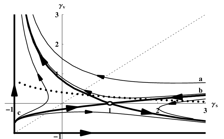
Figure 1: The projection of the RG flow in the three dimensional parameter space (σx​x,γv,γs)(\sigma_{xx},\gamma_{v},\gamma_{s}) onto (γv,γs)(\gamma_{v},\gamma_{s}) plane for the S​U​(2)×S​U​(2)SU(2)\times SU(2) symmetry case (Eqs. (62)-(64)). Dots denote the line at which 1+6​f​(γv)+f⁡(γs)=01+6f(\gamma_{v})+f(\gamma_{s})=0. The dashed line indicates the line γv=γs\gamma_{v}=\gamma_{s} (see text).
Refer to caption
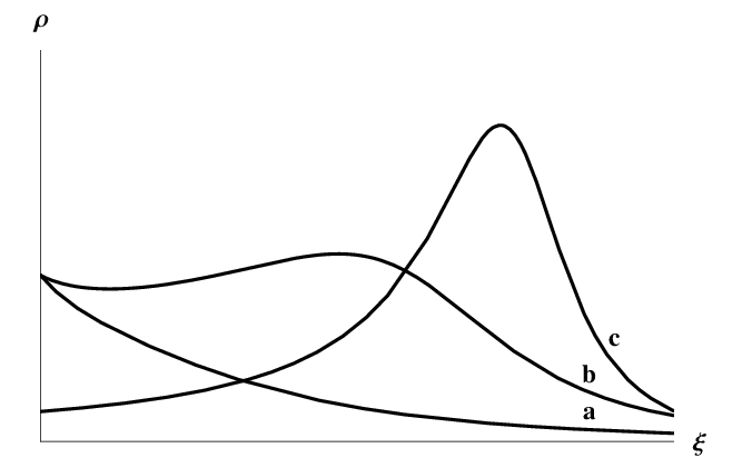
Figure 2: Schematic dependence of the resistance ρ=1/(π​σx​x)\rho=1/(\pi\sigma_{xx}) on ξ\xi. Curves aa, bb, and cc corresponds to the flow lines aa, bb, and cc in Fig. 1 (see text).

IV.4 One loop RG equations

Using the standard method, [30] we derive from Eqs. (58), (60) and (61) one-loop results for the RG equations which determine the T=0T=0 behavior of the physical observables with changing the length scale LL. It is convenient to define γv=Γ2/z\gamma_{v}=\Gamma_{2}/z and γs=−1+4​Γ+⁣−/z\gamma_{s}=-1+4\Gamma_{+-}/z. Then, for 𝔻=2\mathbb{D}=2 we obtain

d​σx​xd​ξ=−2π​[1+6​f​(γv)+f⁡(γs)]\displaystyle\frac{d\sigma_{xx}}{d\xi}=-\frac{2}{\pi}\left[1+6f(\gamma_{v})+f(\gamma_{s})\right] (62)
d​γvd​ξ=1+γvπ​σx​x​(1+2​γv−γs)\displaystyle\frac{d\gamma_{v}}{d\xi}=\frac{1+\gamma_{v}}{\pi\sigma_{xx}}(1+2\gamma_{v}-\gamma_{s}) (63)
d​γsd​ξ=1+γsπ​σx​x​(1−6​γv−γs)\displaystyle\frac{d\gamma_{s}}{d\xi}=\frac{1+\gamma_{s}}{\pi\sigma_{xx}}(1-6\gamma_{v}-\gamma_{s}) (64)
d​ln⁡zd​ξ=−1π​σx​x​[1−6​γv−γs].\displaystyle\frac{d\ln z}{d\xi}=-\frac{1}{\pi\sigma_{xx}}\left[1-6\gamma_{v}-\gamma_{s}\right]. (65)

Eqs. (62)-(65) constitute one of the main results of the present paper and describe the system at the intermediate length scales Ls≪L≪LvL_{s}\ll L\ll L_{v}. We mention that the length scale ll involved in ξ=ln⁡L/l\xi=\ln L/l is now of the order of LsL_{s}.

In Figure 1 we present the projection of the RG flow in the three dimensional parameter space (σx​x,γv,γs)(\sigma_{xx},\gamma_{v},\gamma_{s}) onto (γv,γs)(\gamma_{v},\gamma_{s}) plane. There is the unstable fixed point at γv=0\gamma_{v}=0 and γs=1\gamma_{s}=1. However, for the physical system considered the fixed point is inaccessible since an initial point of the RG flow is always situated near the line γv=γs\gamma_{v}=\gamma_{s}. As shown in Fig. 2, there are possible three distinct types of the ρ⁡(ξ)\rho(\xi) behavior for such initial points. Along the RG flow line aa (Fig. 1) that crosses the curve dd described by the equation 1+6​f​(γv)+f⁡(γs)=01+6f(\gamma_{v})+f(\gamma_{s})=0 the resistance demonstrates the metallic behavior: ρ\rho decreases as ξ\xi grows. If we move along the RG flow line bb which intersects the curve dd twice, then the resistance develops the minimum and the maximum. At last, the resistance on the RG flow line cc which has single crossing with the curve dd has the maximum. Remarkably, in all three cases, the behavior of the resistance is of the metallic type for relatively large LL. The reason of this metallic behavior can be understood from the following arguments. At large ξ\xi, the coupling γv\gamma_{v} flows to large positive values whereas γs→−1\gamma_{s}\to-1. Then, Γ+⁣−/Γ+⁣+∼1/γv≪1\Gamma_{+-}/\Gamma_{++}\sim 1/\gamma_{v}\ll 1 and the RG Eqs. (62)-(65) transforms into equations for the single valley system with the conductance equal σx​x/2\sigma_{xx}/2. The metallic behavior of this system is well-known. [5]

V Completely symmetry broken case

V.1 Effective action

At the long length scales L≫LvL\gg L_{v} the symmetry breaking term 𝒮v​b\mathcal{S}_{vb} becomes important. In the quadratic approximation it reads

𝒮v​b=i​zv​Δv2​∫d2​𝐫​∑nj,τjαj,σ(τ2−τ1)​[wn1​n2;τ1​τ2α1​α2]σ​[w¯n2​n1;τ2​τ1α2​α1]σ.\mathcal{S}_{vb}=\frac{iz_{v}\Delta_{v}}{2}\int d^{2}\mathbf{r}\sum^{\alpha_{j},\sigma}_{n_{j},\tau_{j}}\left(\tau_{2}-\tau_{1}\right)[w_{n_{1}n_{2};\tau_{1}\tau_{2}}^{\alpha_{1}\alpha_{2}}]_{\sigma}[\bar{w}_{n_{2}n_{1};\tau_{2}\tau_{1}}^{\alpha_{2}\alpha_{1}}]_{\sigma}. (66)

Hence, the modes in [Qn​m;τ1​τ2α​β]σ[Q^{\alpha\beta}_{nm;\tau_{1}\tau_{2}}]_{\sigma} with τ1≠τ2\tau_{1}\neq\tau_{2} acquire a finite mass of the order of zv​Δvz_{v}\Delta_{v}. Therefore, they are negligible at long length scales L≫LvL\gg L_{v}. As the result, the matrix QQ becomes diagonal matrix in the valley isospin space. The valley susceptibility remains constant under the action of the renormalization group on these length scales:

d​zvd​ξ=0,L≫Lv.\frac{dz_{v}}{d\xi}=0,\qquad L\gg L_{v}. (67)

Let us define

Qjα​β={[Q11α​β]+,[Q−1−1α​β]+,[Q11α​β]−,[Q−1−1α​β]−}.Q_{j}^{\alpha\beta}=\{[Q_{11}^{\alpha\beta}]_{+},[Q_{-1-1}^{\alpha\beta}]_{+},[Q_{11}^{\alpha\beta}]_{-},[Q_{-1-1}^{\alpha\beta}]_{-}\}. (68)

Then the action 𝒮=𝒮σ+𝒮F\mathcal{S}=\mathcal{S}_{\sigma}+\mathcal{S}_{F} reads

𝒮σ=−σx​x32∑j∫d2𝐫tr(∇Qj)2\mathcal{S}_{\sigma}=-\frac{\sigma_{xx}}{32}\sum_{j}\int d^{2}\mathbf{r}\tr(\nabla Q_{j})^{2} (69)

and

𝒮F=π​T​∫d2​𝐫​∑j,k∑α​ntr⁡Inα​Qj​Γ^j​k​tr​I−nα​Qk\displaystyle\mathcal{S}_{F}=\pi T\int d^{2}\mathbf{r}\sum_{j,k}\sum_{\alpha n}\tr I_{n}^{\alpha}Q_{j}\hat{\Gamma}_{jk}\tr I_{-n}^{\alpha}Q_{k} (70)
+4πTz∑j∫d2𝐫trηQj,\displaystyle+4\pi Tz\sum_{j}\int d^{2}\mathbf{r}\tr\eta Q_{j}, (71)

where

Γ^=(Γ+⁣+−Γ2Γ~+⁣+Γ~+⁣−Γ+⁣−Γ~+⁣+Γ+⁣+−Γ2Γ+⁣−Γ~+⁣−Γ~+⁣−Γ+⁣−Γ+⁣+−Γ2Γ~+⁣+Γ+⁣−Γ~+⁣−Γ~+⁣+Γ+⁣+−Γ2).\displaystyle\hat{\Gamma}=\begin{pmatrix}\Gamma_{++}-\Gamma_{2}&\tilde{\Gamma}_{++}&\tilde{\Gamma}_{+-}&\Gamma_{+-}\\ \tilde{\Gamma}_{++}&\Gamma_{++}-\Gamma_{2}&\Gamma_{+-}&\tilde{\Gamma}_{+-}\\ \tilde{\Gamma}_{+-}&\Gamma_{+-}&\Gamma_{++}-\Gamma_{2}&\tilde{\Gamma}_{++}\\ \Gamma_{+-}&\tilde{\Gamma}_{+-}&\tilde{\Gamma}_{++}&\Gamma_{++}-\Gamma_{2}\end{pmatrix}. (72)

Initially, at the length scale of the order of LvL_{v}, the coupling Γ~+⁣+=Γ+⁣+\tilde{\Gamma}_{++}=\Gamma_{++} and Γ~+⁣−=Γ+⁣−\tilde{\Gamma}_{+-}=\Gamma_{+-}. However, more general structure (72) is consistent with the renormalization group. It is worthwhile to mention that if the matrix Γ^\hat{\Gamma} is diagonal then the theory (69) and (71) would include four copies of the singlet U⁡(1)U(1) theory studied in Refs. [7, 8]. The action (71) corresponds to the following low energy part of the electron-electron interaction Hamiltonian:

ℋint=12​∫d​𝐫​∑σ​σ′;τ​τ′ρτσ​[(Γs)τ​τ′σ​σ′+Γt​(ta)τ​τσ​σ​(ta)τ′​τ′σ′​σ′]​ρτσ\displaystyle\mathcal{H}_{\textrm{int}}=\frac{1}{2}\int d\mathbf{r}\sum_{\sigma\sigma^{\prime};\tau\tau^{\prime}}\rho^{\sigma}_{\tau}\Bigl[(\Gamma_{s})_{\tau\tau^{\prime}}^{\sigma\sigma^{\prime}}+\Gamma_{t}(t^{a})^{\sigma\sigma}_{\tau\tau}(t^{a})^{\sigma^{\prime}\sigma^{\prime}}_{\tau^{\prime}\tau^{\prime}}\Bigr]\rho^{\sigma}_{\tau}
ρτσ=ψ¯τσ​ψτσ\displaystyle\rho^{\sigma}_{\tau}=\bar{\psi}^{\sigma}_{\tau}\psi^{\sigma}_{\tau} (73)

In order to have the invariance under the global rotations

Qj→ei​χ^​Qj​e−i​χ^,χ^=∑α​nχnα​Inα,\displaystyle Q_{j}\to e^{i\hat{\chi}}Q_{j}e^{-i\hat{\chi}},\qquad\hat{\chi}=\sum_{\alpha n}\chi^{\alpha}_{n}I^{\alpha}_{n}, (74)

the following relation has to be fulfilled

z+Γ2−Γ+⁣+−Γ~+⁣+=Γ+⁣−+Γ~+⁣−.\displaystyle z+\Gamma_{2}-\Gamma_{++}-\tilde{\Gamma}_{++}=\Gamma_{+-}+\tilde{\Gamma}_{+-}. (75)

V.2 Perturbative expansions

As above, in order to resolve the constraints Qj2=1Q_{j}^{2}=1, we shall use the “square-root” parameterization for each QjQ_{j}: Qj=Wj+Λ​1−Wj2Q_{j}=W_{j}+\Lambda\sqrt{1-W_{j}^{2}}. Then, the propagators are defined by the theory (69) and (71) as

⟨[wn1​n2α1​α2​(q)]j​[wn4​n3†α4​α3;τ4​τ3​(−q)]k⟩=32σx​x​𝒟^j​k,\displaystyle\langle[w_{n_{1}n_{2}}^{\alpha_{1}\alpha_{2}}(q)]_{j}[w_{n_{4}n_{3}}^{{\dagger}\alpha_{4}\alpha_{3};\tau_{4}\tau_{3}}(-q)]_{k}\rangle=\frac{32}{\sigma_{xx}}\hat{\mathcal{D}}_{jk}, (76)
𝒟^=δα1​α3δα2​α4δn12,n34[δn1,n3Dq(ω12)+32​π​Tσx​xΓ^δα1​α2\displaystyle\hat{\mathcal{D}}=\delta^{\alpha_{1}\alpha_{3}}\delta^{\alpha_{2}\alpha_{4}}\delta_{n_{12},n_{34}}\Bigl[\delta_{n_{1},n_{3}}D_{q}(\omega_{12})+\frac{32\pi T}{\sigma_{xx}}\hat{\Gamma}\delta^{\alpha_{1}\alpha_{2}}
×Dq(ω12)D^qc(ω12)],\displaystyle\times D_{q}(\omega_{12})\hat{D}^{c}_{q}(\omega_{12})\Bigr], (77)

where

[D^qc​(ωn)]−1=q2+16σx​x​(z−Γ^)​ωn.\displaystyle[\hat{D}^{c}_{q}(\omega_{n})]^{-1}=q^{2}+\frac{16}{\sigma_{xx}}(z-\hat{\Gamma})\omega_{n}. (78)

The conservation of the zz-components of the total spin, ∑σ​τσ​ρτσ\sum_{\sigma\tau}\sigma\rho_{\tau}^{\sigma}, and the total valley isospin, ∑σ​ττ​ρτσ\sum_{\sigma\tau}\tau\rho_{\tau}^{\sigma}, implies (see Eq. (31)) that zs=2​Γ+⁣−+2​Γ~+⁣−z_{s}=2\Gamma_{+-}+2\tilde{\Gamma}_{+-} and zv=2​Γ~+⁣++2​Γ~+⁣−z_{v}=2\tilde{\Gamma}_{++}+2\tilde{\Gamma}_{+-}. Since, for L≫LvL\gg L_{v} both zsz_{s} and zvz_{v} are not renormalized, we obtain

d​Γ~+⁣−d​ξ=d​Γ+⁣−d​ξ=d​Γ~+⁣+d​ξ=0.\displaystyle\frac{d\tilde{\Gamma}_{+-}}{d\xi}=\frac{d\Gamma_{+-}}{d\xi}=\frac{d\tilde{\Gamma}_{++}}{d\xi}=0. (79)

Since, both Γ~+⁣−\tilde{\Gamma}_{+-} and Γ+⁣−\Gamma_{+-} coincides at the length scales L∼LvL\sim L_{v} and they are not renormalized we shall not distinguish Γ~+⁣−\tilde{\Gamma}_{+-} and Γ+⁣−\Gamma_{+-} from here onwards. If we introduce γs\gamma_{s} and γv\gamma_{v} such that Γ+⁣−=Γ~+⁣−=z⁡(1+γs)/4\Gamma_{+-}=\tilde{\Gamma}_{+-}=z(1+\gamma_{s})/4 and Γ~+⁣+=z⁡(1+2​γv−γs)/4\tilde{\Gamma}_{++}=z(1+2\gamma_{v}-\gamma_{s})/4 then both γs\gamma_{s} and γv\gamma_{v} coincide with the corresponding couplings of the previous sections at the length scales L∼LvL\sim L_{v}.

V.3 One-loop approximation

Evaluating the conductivity with the help of Eq. (23) in the one-loop approximation, we find

σx​x′​(i​ωn)=σx​x+28​π𝔻​σx​x​∫pp2​T​∑ωm>0min⁡{ωmωn,1}\displaystyle\sigma^{\prime}_{xx}(i\omega_{n})=\sigma_{xx}+\frac{2^{8}\pi}{\mathbb{D}\sigma_{xx}}\int_{p}p^{2}T\sum_{\omega_{m}>0}\min\left\{\frac{\omega_{m}}{\omega_{n}},1\right\}
Dp​(ωm+ωn)​Dp​(ωm)​∑j(Γ^​D^pc​(ωm))j​j.\displaystyle D_{p}(\omega_{m}+\omega_{n})D_{p}(\omega_{m})\sum_{j}\left(\hat{\Gamma}\hat{D}^{c}_{p}(\omega_{m})\right)_{jj}. (80)

Hence,

σx​x′​(i​ωn)=σx​x+28​π​z𝔻​σx​x​∫pp2​T​∑ωm>0min⁡{ωmωn,1}\displaystyle\sigma^{\prime}_{xx}(i\omega_{n})=\sigma_{xx}+\frac{2^{8}\pi z}{\mathbb{D}\sigma_{xx}}\int_{p}p^{2}T\sum_{\omega_{m}>0}\min\left\{\frac{\omega_{m}}{\omega_{n}},1\right\}
Dp​(ωm+ωn)​Dp​(ωm)​[Dps​(ωm)−2​γv​D¯pt​(ωm)−γs​D~pt​(ωm)]\displaystyle D_{p}(\omega_{m}+\omega_{n})D_{p}(\omega_{m})\left[{D}^{s}_{p}(\omega_{m})-2\gamma_{v}\bar{D}^{t}_{p}(\omega_{m})-\gamma_{s}\tilde{D}^{t}_{p}(\omega_{m})\right] (81)

where

[D¯qt​(ωn)]−1=q2+32σx​x​(Γ+⁣++Γ~+⁣+)​ωn.\displaystyle[\bar{D}^{t}_{q}(\omega_{n})]^{-1}=q^{2}+\frac{32}{\sigma_{xx}}(\Gamma_{++}+\tilde{\Gamma}_{++})\omega_{n}. (82)

Performing the analytic continuation to the real frequencies in Eq. (81), we find

σx​x′=σx​x−28​π​z𝔻​σx​x∫pp2∫0∞dωDp2(ω)[Dps(ω)\displaystyle\sigma^{\prime}_{xx}=\sigma_{xx}-\frac{2^{8}\pi z}{\mathbb{D}\sigma_{xx}}\int_{p}p^{2}\int_{0}^{\infty}d\omega D^{2}_{p}(\omega)\Bigl[{D}^{s}_{p}(\omega)
−2γvD¯pt(ω)−γsD~pt(ω)].\displaystyle\hskip 28.45274pt-2\gamma_{v}\bar{D}^{t}_{p}(\omega)-\gamma_{s}\tilde{D}^{t}_{p}(\omega)\Bigr]. (83)

As in the previous Section, in order to compute z′z^{\prime} we evaluate the thermodynamic potential in the one-loop approximation. The result is

T2∂Ω/T∂T=8TNrz∑ωn>0ωn[1+8σx​x∫p[(1+γs)2D~pt(ωn)\displaystyle T^{2}\frac{\partial\Omega/T}{\partial T}=8TN_{r}z\sum_{\omega_{n}>0}\omega_{n}\Bigl[1+\frac{8}{\sigma_{xx}}\int_{p}\Bigl[\frac{(1+\gamma_{s})}{2}\tilde{D}_{p}^{t}(\omega_{n})
+(1+γv)D¯pt(ωn)−2Dp(ωn)]].\displaystyle+(1+\gamma_{v})\bar{D}_{p}^{t}(\omega_{n})-2D_{p}(\omega_{n})\Bigr]\Bigr]. (84)

Hence, we obtain

z′=z+16σx​x​(Γ2−Γ+⁣+)​∫pDp​(0).\displaystyle z^{\prime}=z+\frac{16}{\sigma_{xx}}(\Gamma_{2}-\Gamma_{++})\int_{p}D_{p}(0). (85)

We mention [29] that the results (79),  (83), and (85) can be obtained with the help of the background field procedure applied to the action (69)-(71).

Refer to caption
Figure 3: The projection of the RG flow in the three dimensional parameter space (σx​x,γv,γs)(\sigma_{xx},\gamma_{v},\gamma_{s}) onto (γv,γs)(\gamma_{v},\gamma_{s}) plane for the completely symmetry broken case (Eqs. (86)-(88)). Dots denote the line at which 1+2​f​(γv)+f⁡(γs)=01+2f(\gamma_{v})+f(\gamma_{s})=0 (see text).
Refer to caption
Figure 4: Schematic dependence of the resistance ρ=1/(π​σx​x)\rho=1/(\pi\sigma_{xx}) on ξ\xi along the flow line aa in Fig. 3 (see text).

V.4 One loop RG equations

Equations (79), (83) and (85) allow us to derive the following one-loop results for the renormalization group functions which determine the T=0T=0 behavior of the physical observables with changing the length scale LL (𝔻=2\mathbb{D}=2):

d​σx​xd​ξ=−2π​[1+2​f​(γv)+f⁡(γs)]\displaystyle\frac{d\sigma_{xx}}{d\xi}=-\frac{2}{\pi}\left[1+2f(\gamma_{v})+f(\gamma_{s})\right] (86)
d​γvd​ξ=1+γvπ​σx​x​(1−2​γv−γs)\displaystyle\frac{d\gamma_{v}}{d\xi}=\frac{1+\gamma_{v}}{\pi\sigma_{xx}}(1-2\gamma_{v}-\gamma_{s}) (87)
d​γsd​ξ=1+γsπ​σx​x​(1−2​γv−γs)\displaystyle\frac{d\gamma_{s}}{d\xi}=\frac{1+\gamma_{s}}{\pi\sigma_{xx}}(1-2\gamma_{v}-\gamma_{s}) (88)
d​ln⁡zd​ξ=−1π​σx​x​[1−2​γv−γs]\displaystyle\frac{d\ln z}{d\xi}=-\frac{1}{\pi\sigma_{xx}}\left[1-2\gamma_{v}-\gamma_{s}\right] (89)

The renormalization group equations (86)-(89) constitute one of the main results of the present paper. We mention that the length scale ll involved in ξ=ln⁡L/l\xi=\ln L/l is now of the order of LvL_{v} and Eqs. (86)-(89) describe the system at the long length scales L≫LvL\gg L_{v}.

The projection of the RG flow for Eqs. (86)-(88) on the γv\gamma_{v} – γs\gamma_{s} plane is shown in Fig. 3. There exits the line of the fixed points that is described by the equation 2​γv+γs=12\gamma_{v}+\gamma_{s}=1. If the initial point has large γv\gamma_{v} or γs\gamma_{s} then the RG flow line crosses the curve that is determined by the condition 1+2​f​(γv)+f⁡(γs)=01+2f(\gamma_{v})+f(\gamma_{s})=0. Therefore, the ρ⁡(ξ)\rho(\xi) dependence along the RG flow line develops the minimum and will be of the insulating type as is shown in Fig. 4.

VI Discussions and conclusions

The renormalization group equations discussed above describe the T=0T=0 behavior of the observable parameters with changing of the length scale LL. At finite temperatures T≫σx​x/(z​Ls​a​m​p​l​e2)T\gg\sigma_{xx}/(zL^{2}_{sample}) where Ls​a​m​p​l​eL_{sample} is the sample size, the temperature behavior of the physical observables can be found from the RG equations stopped at the inelastic length LinL_{\textrm{in}} rather than at the sample size. Formally, it means that one should substitute ξT=12​ln⁡σx​x/(z​T​l2)\xi_{T}=\frac{1}{2}\ln\sigma_{xx}/(zTl^{2}) for ξ\xi in the RG equations with ξT\xi_{T} obeying the following equation [31]

d​ξTd​ξ=1−12​d​ln⁡zd​ξ.\frac{d\xi_{T}}{d\xi}=1-\frac{1}{2}\frac{d\ln z}{d\xi}. (90)

Having in mind Eq. (90), we find that the TT-behavior of the resistivity at B=0B=0 is described by Eqs. (36) and (37) for T≫ΔvT\gg\Delta_{v} and Eqs. (62)-(64) with interchanged γv\gamma_{v} and γs\gamma_{s} for T≪ΔvT\ll\Delta_{v}. In what follows, we assume that Δv<Tmax(I)\Delta_{v}<T_{\textrm{max}}^{(I)} where Tmax(I)T_{\textrm{max}}^{(I)} denotes the temperature of the maximum point that appears in ρ⁡(T)\rho(T) according to the RG Eqs. (36) and (37). Our assumption is consistent with the experimental data in Si-MOSFET where, for example, [32] the valley splitting is of the order of hundreds of m​KmK and Tmax(I)T_{\textrm{max}}^{(I)} is about several Kelvins [33]. Then, depending on the initial conditions at T∼1/τT\sim 1/\tau two types of the ρ⁡(T)\rho(T) behavior are possible as is shown in Fig. 5. The curve aa represents the typical ρ⁡(T)\rho(T) dependence that was observed in transport experiments on two-valley 2D electron systems in Si-MOS samples [2] and n-AlAs quantum well. [34] Surprisingly, the other behavior with the two maximum points is possible, as illustrated by curve bb in Fig. 5. So far, this interesting non-monotonic ρ⁡(T)\rho(T) dependence has been neither observed experimentally nor predicted theoretically. At very low temperatures T≪ΔvT\ll\Delta_{v}, the metallic behavior of ρ⁡(T)\rho(T) wins even in the presence of the valley splitting.

Refer to caption
Figure 5: The schematic ρ⁡(T)\rho(T) dependence in the case of zero parallel magnetic field. See text

In the presence of the sufficiently low parallel magnetic field Δs<Tmax(I)\Delta_{s}<T_{\textrm{max}}^{(I)}, the ρ⁡(T)\rho(T) behavior of three distinct types is possible as plotted in Fig. 6. In all three cases, the ρ⁡(T)\rho(T) dependence has the maximum point at temperature T=Tmax(I)T=T_{\textrm{max}}^{(I)} and is of the insulating type as T→0T\to 0. As follows from Fig. 2, in the intermediate temperature range, when TT is between Δs\Delta_{s} and Δv\Delta_{v}, the metallic (curve aa), insulating (curve bb) and nonmonotonic (curve cc) types of the ρ⁡(T)\rho(T) behavior emerge. As a result, there has to exist the ρ⁡(T)\rho(T) dependence with two maximum points in the presence of BB.

Refer to caption
Figure 6: The schematic ρ⁡(T)\rho(T) dependence in the presence of both spin and valley splitting in the case Δs<Δv\Delta_{s}<\Delta_{v}. For the opposite case, the behavior will be similar. See text

For high magnetic fields such that Δs>Tmax(I)\Delta_{s}>T_{\textrm{max}}^{(I)} the maximum point at T=Tmax(I)T=T_{\textrm{max}}^{(I)} is absent, and two types of the ρ⁡(T)\rho(T) behavior are possible as is shown in Fig. 7. If Tmax(I​I)<ΔvT_{\textrm{max}}^{(II)}<\Delta_{v}, then the dependence of the resistivity is monotonic and insulating, see the curve aa in Fig. 7. Here, Tmax(I​I)T_{\textrm{max}}^{(II)} denotes the temperature of the maximum point that appears in the resistivity in accord with the RG Eqs. (62) and (63). In the opposite case Tmax(I​I)>ΔvT_{\textrm{max}}^{(II)}>\Delta_{v}, a typical ρ⁡(T)\rho(T) dependence is illustrated by the curve bb in Fig. 7. Therefore, if the valley splitting is sufficiently large, i.e., Δv>Tmax(I​I)\Delta_{v}>T_{\textrm{max}}^{(II)}, then the monotonic insulating behavior of the resistivity appears in the parallel magnetic field which corresponds to Δs∼Tmax(I)\Delta_{s}\sim T_{\textrm{max}}^{(I)}. This is the case for the experiments on the magnetotransport in Si-MOSFET. [10, 33] However, if the valley splitting is small, Δv<Tmax(I​I)\Delta_{v}<T_{\textrm{max}}^{(II)}, then the maximum point of the ρ⁡(T)\rho(T) dependence survives even in high magnetic fields but shifts down to lower temperatures.

Refer to caption
Figure 7: The schematic ρ⁡(T)\rho(T) dependence in the presence of strong parallel magnetic field: Δv,Tmax(I)<Δs\Delta_{v},T_{\textrm{max}}^{(I)}<\Delta_{s}. See text

In addition, to interesting TT-dependences of the resistivity, the theory predicts strong renormalization of the electron-electron interaction with temperature. In order to characterize this renormalization, we consider the ratio χv/χs\chi_{v}/\chi_{s} of valley and spin susceptibilities. In Figure 8, we present the schematic dependence of χv/χs\chi_{v}/\chi_{s} on TT for a fixed valley splitting but with varying spin splitting. At high temperatures, T≫Δv,ΔsT\gg\Delta_{v},\Delta_{s} the ratio of the susceptibilities equals unity, χv/χs=1\chi_{v}/\chi_{s}=1. At low temperatures, T≪Δv,ΔsT\ll\Delta_{v},\Delta_{s}, we find

χvχs={<1,Δs<Δv1,Δs=Δv>1,Δs>Δv.\frac{\chi_{v}}{\chi_{s}}=\begin{cases}<1&,\,\Delta_{s}<\Delta_{v}\\ 1&,\,\Delta_{s}=\Delta_{v}\\ >1&,\,\Delta_{s}>\Delta_{v}.\end{cases} (91)

Therefore, the ratio χv/χs\chi_{v}/\chi_{s} at T→0T\to 0 is sensitive to the ratio Δv/Δs\Delta_{v}/\Delta_{s}. This can be used for the experimental determination of the valley splitting in the 2D electron system.

Finally, we remind that we do not consider above the contribution to the one-loop RG equations from the particle-particle (Cooper) channel. It can be shown (see Appendix) that neither the spin splitting nor the valley splitting does not change the “cooperon” contribution to the RG equations in the one-loop approximation. Therefore, the Cooper-channel contribution to the RG equations discussed above can be taken into account by the substitution of 1+21+2 for 11 in the square brackets of Eqs. (36), (62) and (86). The Cooper-channel contribution does not change qualitative behavior of the resistivity, and the valley and spin susceptibilities discussed above.

Refer to caption
Figure 8: The schematic dependence of the ration χv/χs\chi_{v}/\chi_{s} on temperature: a) for Δs<Δv\Delta_{s}<\Delta_{v}; b) for Δs=Δv\Delta_{s}=\Delta_{v}; c) for Δs>Δv\Delta_{s}>\Delta_{v}. The temperature scales Ta,c≡ΔsT_{a,c}\equiv\Delta_{s}.

To summarize, we have obtained the novel results on the temperature behavior of such physical observables as the resistivity, spin and valley susceptibilities in 2D electron liquid with two valleys in the MIT vicinity and in the presence of both the parallel magnetic field and the valley splitting. First, we found that the metallic behavior of the resistivity at low temperatures survives in the presence of only the parallel magnetic field or the valley splitting. If both the spin splitting and the valley splitting exist then the metallic ρ\rho-dependence crosses over to insulating one at low temperatures. Second, we have predicted the existence of the novel, nonmonotonic dependence of resistivity at zero and finite magnetic field in which the ρ⁡(T)\rho(T) has two maximum points. It would be an experimental challenge to identify this novel regime.

Acknowledgements.
The authors are grateful to D.A. Knyazev, A.A. Kuntzevich, O.E. Omelyanovsky, and V.M. Pudalov for the detailed discussions of their experimental data. The research was funded in part by CRDF, the Russian Ministry of Education and Science, Council for Grants of the President of Russian Federation, RFBR 07-02-00998-a and 06-02-16708-a, Dynasty Foundation, Programs of RAS, and Russian Science Support Foundation.

Appendix A “Cooperon” contribution to the conductance

We start from the standard equation for the “cooperon”

Cσ3​σ4;τ3​τ4σ1​σ2;τ1​τ2​(q)=δσ1,σ2​δτ1,τ2​δσ3,σ4​δτ3,τ4​12​π​ν​τi\displaystyle C^{\sigma_{1}\sigma_{2};\tau_{1}\tau_{2}}_{\sigma_{3}\sigma_{4};\tau_{3}\tau_{4}}(q)=\delta^{\sigma_{1},\sigma_{2}}\delta^{\tau_{1},\tau_{2}}\delta^{\sigma_{3},\sigma_{4}}\delta^{\tau_{3},\tau_{4}}\frac{1}{2\pi\nu\tau_{i}}
+Iσ3​σ6;τ3​τ6σ1​σ5;τ1​τ5​(q)​Cσ6​σ4;τ6​τ4σ5​σ2;τ5​τ2​(q)\displaystyle+I^{\sigma_{1}\sigma_{5};\tau_{1}\tau_{5}}_{\sigma_{3}\sigma_{6};\tau_{3}\tau_{6}}(q)C^{\sigma_{5}\sigma_{2};\tau_{5}\tau_{2}}_{\sigma_{6}\sigma_{4};\tau_{6}\tau_{4}}(q) (92)

where the “impurity ladder” is given as

Iσ3​σ4;τ3​τ4σ1,σ2;τ1​τ2​(q)=12​π​ν​τi​∫pGσ1,σ2;τ1​τ2R​(p+)​Gσ3​σ4;τ3​τ4A​(p−)\displaystyle I^{\sigma_{1},\sigma_{2};\tau_{1}\tau_{2}}_{\sigma_{3}\sigma_{4};\tau_{3}\tau_{4}}(q)=\frac{1}{2\pi\nu\tau_{i}}\int_{p}G^{R}_{\sigma_{1},\sigma_{2};\tau_{1}\tau_{2}}(p_{+})G^{A}_{\sigma_{3}\sigma_{4};\tau_{3}\tau_{4}}(p_{-}) (93)

Here, p±=p±q/2p_{\pm}=p\pm q/2 and the impurity averaged Green functions are given as

[Gσ1,σ2;τ1​τ2R⁡(A)(p)]−1=δσ1,σ2δτ1​τ2[p22​me−μ+Δssgnσ1\displaystyle[G^{R(A)}_{\sigma_{1},\sigma_{2};\tau_{1}\tau_{2}}(p)]^{-1}=\delta^{\sigma_{1},\sigma_{2}}\delta^{\tau_{1}\tau_{2}}\Bigl[\frac{p^{2}}{2m_{e}}-\mu+\Delta_{s}\sgn\sigma_{1}
+Δvsgnτ1±i/2τi].\displaystyle\hskip 56.9055pt+\Delta_{v}\sgn\tau_{1}\pm i/2\tau_{i}\Bigr]. (94)

Performing integration, we find for q→0q\to 0

Iσ3​σ4;τ3​τ4σ1,σ2;τ1​τ2(q)=δσ1,σ3δσ2​σ4δτ1​τ3δτ2​τ4[1−Dq2τi\displaystyle I^{\sigma_{1},\sigma_{2};\tau_{1}\tau_{2}}_{\sigma_{3}\sigma_{4};\tau_{3}\tau_{4}}(q)=\delta^{\sigma_{1},\sigma_{3}}\delta^{\sigma_{2}\sigma_{4}}\delta^{\tau_{1}\tau_{3}}\delta^{\tau_{2}\tau_{4}}\Bigl[1-Dq^{2}\tau_{i}
−iΔsτi(sgnσ3−sgnσ1)−iΔvτi(sgnτ3−sgnτ1)].\displaystyle-i\Delta_{s}\tau_{i}(\sgn\sigma_{3}-\sgn\sigma_{1})-i\Delta_{v}\tau_{i}(\sgn\tau_{3}-\sgn\tau_{1})\Bigr]. (95)

Next, solving Eq. (92), we obtain

Cσ3​σ4;τ3​τ4σ1,σ2;τ1​τ2(q)=δσ1​σ2δσ3​σ4δτ1​τ2δτ3​τ412​π​ν​τi2[Dq2\displaystyle C^{\sigma_{1},\sigma_{2};\tau_{1}\tau_{2}}_{\sigma_{3}\sigma_{4};\tau_{3}\tau_{4}}(q)=\delta^{\sigma_{1}\sigma_{2}}\delta^{\sigma_{3}\sigma_{4}}\delta^{\tau_{1}\tau_{2}}\delta^{\tau_{3}\tau_{4}}\frac{1}{2\pi\nu\tau_{i}^{2}}\Bigl[Dq^{2} (96)
+iΔs(sgnσ3−sgnσ1)+iΔv(sgnτ3−sgnτ1)]−1\displaystyle+i\Delta_{s}(\sgn\sigma_{3}-\sgn\sigma_{1})+i\Delta_{v}(\sgn\tau_{3}-\sgn\tau_{1})\Bigr]^{-1}

The interference correction to the conductance is given as

δσx​x=−Dτi∫pGR(−p)σ3​σ4;τ3​τ4Gσ4​σ5;τ4​τ5A(−p)\displaystyle\delta\sigma_{xx}=-\frac{D}{\tau_{i}}\int_{p}G^{R}(-p)_{\sigma_{3}\sigma_{4};\tau_{3}\tau_{4}}G^{A}_{\sigma_{4}\sigma_{5};\tau_{4}\tau_{5}}(-p) (97)
×Gσ1​σ2;τ1​τ2R​(p)​Gσ6​σ1;τ6​τ1A​(p)​∫d2​q(2​π)2​Cσ5​σ6;τ5​τ6σ2​σ3;τ2​τ3​(q).\displaystyle\hskip 28.45274pt\times G^{R}_{\sigma_{1}\sigma_{2};\tau_{1}\tau_{2}}(p)G^{A}_{\sigma_{6}\sigma_{1};\tau_{6}\tau_{1}}(p)\int\frac{d^{2}q}{(2\pi)^{2}}C^{\sigma_{2}\sigma_{3};\tau_{2}\tau_{3}}_{\sigma_{5}\sigma_{6};\tau_{5}\tau_{6}}(q).

Using the result:

∫pGR​(−p)σ3​σ4;τ3​τ4​Gσ4​σ5;τ4​τ5A​(−p)​Gσ1​σ2;τ1​τ2R​(p)​Gσ6​σ1;τ6​τ1A​(p)\displaystyle\int_{p}G^{R}(-p)_{\sigma_{3}\sigma_{4};\tau_{3}\tau_{4}}G^{A}_{\sigma_{4}\sigma_{5};\tau_{4}\tau_{5}}(-p)G^{R}_{\sigma_{1}\sigma_{2};\tau_{1}\tau_{2}}(p)G^{A}_{\sigma_{6}\sigma_{1};\tau_{6}\tau_{1}}(p)
=4​π​ν​τi3​δσ3​σ5​δσ2​σ6​δτ3​τ5​δτ2​τ61+Δs2​τi2​(sgn⁡σ2−sgn⁡σ3)2+Δv2​τi2​(sgn⁡τ2−sgn⁡τ3)2,\displaystyle=\frac{4\pi\nu\tau_{i}^{3}\delta^{\sigma_{3}\sigma_{5}}\delta^{\sigma_{2}\sigma_{6}}\delta^{\tau_{3}\tau_{5}}\delta^{\tau_{2}\tau_{6}}}{1+\Delta^{2}_{s}\tau_{i}^{2}(\sgn\sigma_{2}-\sgn\sigma_{3})^{2}+\Delta^{2}_{v}\tau_{i}^{2}(\sgn\tau_{2}-\sgn\tau_{3})^{2}}, (98)

we find

δσx​x=−∑σ1​σ2τ1​τ2δσ1​σ2δτ1​τ2[1+Δs2τi2(sgnσ1−sgnσ2)2\displaystyle\delta\sigma_{xx}=-\sum_{\sigma_{1}\sigma_{2}}^{\tau_{1}\tau_{2}}\delta^{\sigma_{1}\sigma_{2}}\delta^{\tau_{1}\tau_{2}}\Bigl[1+\Delta^{2}_{s}\tau_{i}^{2}(\sgn\sigma_{1}-\sgn\sigma_{2})^{2}
+Δv2τi2(sgnτ1−sgnτ2)2]−1D∫d2​q(2​π)2[Dq2\displaystyle+\Delta^{2}_{v}\tau_{i}^{2}(\sgn\tau_{1}-\sgn\tau_{2})^{2}\Bigr]^{-1}D\int\frac{d^{2}q}{(2\pi)^{2}}\Bigl[Dq^{2}
+iΔs(sgnσ1−sgnσ2)+iΔv(sgnτ1−sgnτ2)]−1\displaystyle+i\Delta_{s}(\sgn\sigma_{1}-\sgn\sigma_{2})+i\Delta_{v}(\sgn\tau_{1}-\sgn\tau_{2})\Bigr]^{-1}
=−4π∫d​qq.\displaystyle=-\frac{4}{\pi}\int\frac{dq}{q}. (99)

Therefore, neither the spin splitting nor the valley splitting affect the Cooper channel (interference) contribution to the conductance.

References

  • [1] T. Ando, A.B. Fowler, and F. Stern, Rev. Mod. Phys. 54, 437 (1982).
  • [2] S.V. Kravchenko, G.V. Kravchenko, J.E. Furneaux, V.M. Pudalov, M. D’Iorio, Phys. Rev. B 50, 8039 (1994).
  • [3] S.V. Kravchenko, W.E. Mason, G.E. Bowker, J.E. Furneaux, V.M. Pudalov, and M.D’Iorio, Phys. Rev. B 51 7038 (1995).
  • [4] E. Abrahams, S.V. Kravchenko, and M.P. Sarachik, Rev. Mod. Phys. 73, 251 (2001); S.V. Kravchenko, and M.P. Sarachik, Rep. Prog. Phys, 67, 1 (2004).
  • [5] A.M. Finkelstein, Electron liquid in disordered conductors, vol. 14 of Soviet Scientific Reviews, ed. by I.M.  Khalatnikov, Harwood Academic Publishers, London, (1990).
  • [6] A. Punnoose, and A.M. Finkelstein, Science 310, 289 (2005).
  • [7] M.A. Baranov, A.M.M. Pruisken, and B. Škorić, Phys. Rev. B 60, 16821 (1999).
  • [8] M. A. Baranov, I. S. Burmistrov, and A. M. M. Pruisken, Phys. Rev. B 66, 075317 (2002).
  • [9] A. Punnoose, and A.M. Finkelstein, Phys. Rev. Lett. 88, 016802 (2001).
  • [10] D. Simonian, S.V. Kravchenko, M.P. Sarachik, and V.M. Pudalov, Phys. Rev. Lett. 79, 2304 (1997).
  • [11] M. Shayegan, E.P. De Poortere, O. Gunawan, Y.P. Shkolnikov, E. Tutuc, and K. Vakili, Phys. Stat. Sol.(b) 243, 3629 (2006).
  • [12] O. Gunawan, Y.P. Shkolnikov, K. Vakili, T. Gokmen, E. P. De Poortere, and M. Shayegan, Phys. Rev. Lett. 97, 186404 (2006).
  • [13] O. Gunawan, T. Gokmen, K. Vakili, M. Padmanabhan, E. P. De Poortere, and M. Shayegan, Nature Phys. 3, 388 (2007).
  • [14] Recently, the ρ⁡(T)\rho(T)-behavior in the presence of parallel magnetic field has been studied in I.S. Burmistrov and N.M. Chtchelkatchev, JETP Lett. 84, 656 (2006). However, due to a mistake we have found the same RG equations as ones given by Eqs. (62), (64) and (65) but with γs=γv\gamma_{s}=\gamma_{v}. This has led us to the erroneous conclusion that in the presence of the parallel magnetic field only the ρ⁡(T)\rho(T)-dependence crosses over from metallic to insulating.
  • [15] S. Brener, S.V. Iordanski, and A. Kashuba, Phys. Rev. B 67, 125309 (2003).
  • [16] A.Yu. Kuntsevich, N.N. Klimov, S.A. Tarasenko, N.S. Averkiev, V.M. Pudalov, H. Kojima, M.E. Gershenson, Phys. Rev. B 75, 195330 (2007).
  • [17] D. Belitz and T.R. Kirkpatrick, Rev. Mod. Phys. 66, 261 (1994).
  • [18] G. Zala, B.N. Narozhny, and I.L. Aleiner, Phys. Rev. B 64, 214204 (2001).
  • [19] C. Castellani, C. Di Castro, P.A. Lee, and M. Ma, Phys. Rev. B 30, 527 (1984).
  • [20] F. Wegner, Z. Phys. B 35, 207 (1979); L. Schaefer and F. Wegner, Z. Phys. B 38, 113 (1980); A.J. McKane and M. Stone, Ann. Phys. (N.Y.) 131, 36 (1981); K.B. Efetov, A.I. Larkin, D.E. Khemel’nitzkii, Sov. Phys. JETP 52, 568 (1980).
  • [21] C. Castellani and C. Di Castro, Phys. Rev. B 34, 5935 (1986).
  • [22] B.L. Altshuler and A.G. Aronov, in Electron-Electron Interactions in Disordered Conductors, ed. A.J. Efros and M. Pollack, Elsevier Science Publishers, North-Holland, 1985.
  • [23] A.M.M. Pruisken, M.A. Baranov, and B. Škorić, Phys. Rev. B 60, 16807 (1999);
  • [24] A. Kamenev and A. Andreev, Phys. Rev. B 60, 2218 (1999).
  • [25] C. Castellani, C. Di Castro, P.A. Lee, M. Ma, S. Sorella, and E. Tabet, Phys. Rev. B 33, 6169 (1986).
  • [26] A.M.M. Pruisken and I.S. Burmistrov, Ann. of Phys. (N.Y.) 322, 1265 (2007).
  • [27] A.E. Meyerovich, JLTP 53, 487 (1983).
  • [28] G. Zala, B.N. Narozhny, I.L. Aleiner, and V.I. Falko, Phys. Rev. B 69, 075306 (2004).
  • [29] I.S. Burmistrov and N.M. Chtchelkatchev, unpublished.
  • [30] D.J. Amit, Field theory, renormalization group, and critical phenomena, (World Scientific, 1984).
  • [31] A.M.M. Pruisken and M.A. Baranov, EuroPhys. Lett. 31, 543 (1995).
  • [32] N. Klimov, M.E. Gershenson, H. Kojima, D.A. Knyazev, V.M. Pudalov, to be published.
  • [33] D.A. Knyazev, O.E. Omel’yanovskii, V.M. Pudalov, and I.S. Burmistrov, JETP Lett. 84, 662 (2006).
  • [34] S.J. Papadakis, and M. Shayegan, Phys. Rev. B 57, R15068 (1998).
  • [35] M.H. Cohen and A.M.M. Pruisken, Phys. Rev. B 49, 4593 (1994).